Region Merging Considering Within- and Between-Segment Heterogeneity: An Improved Hybrid Remote-Sensing Image Segmentation Method

Abstract
:
1. Introduction
2. Materials and Methods
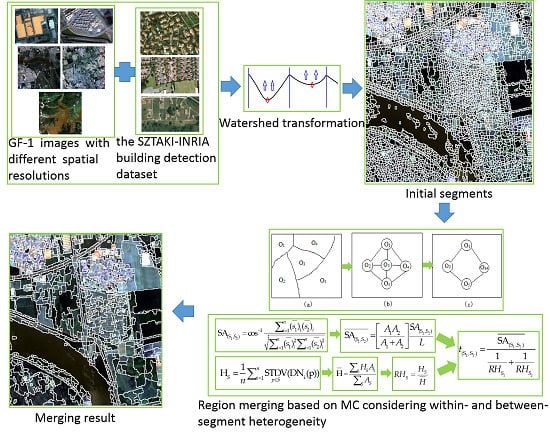
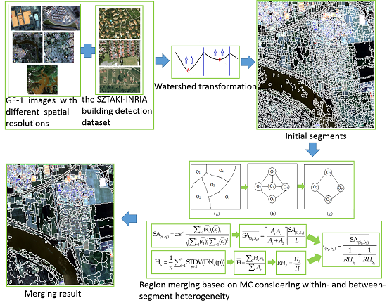
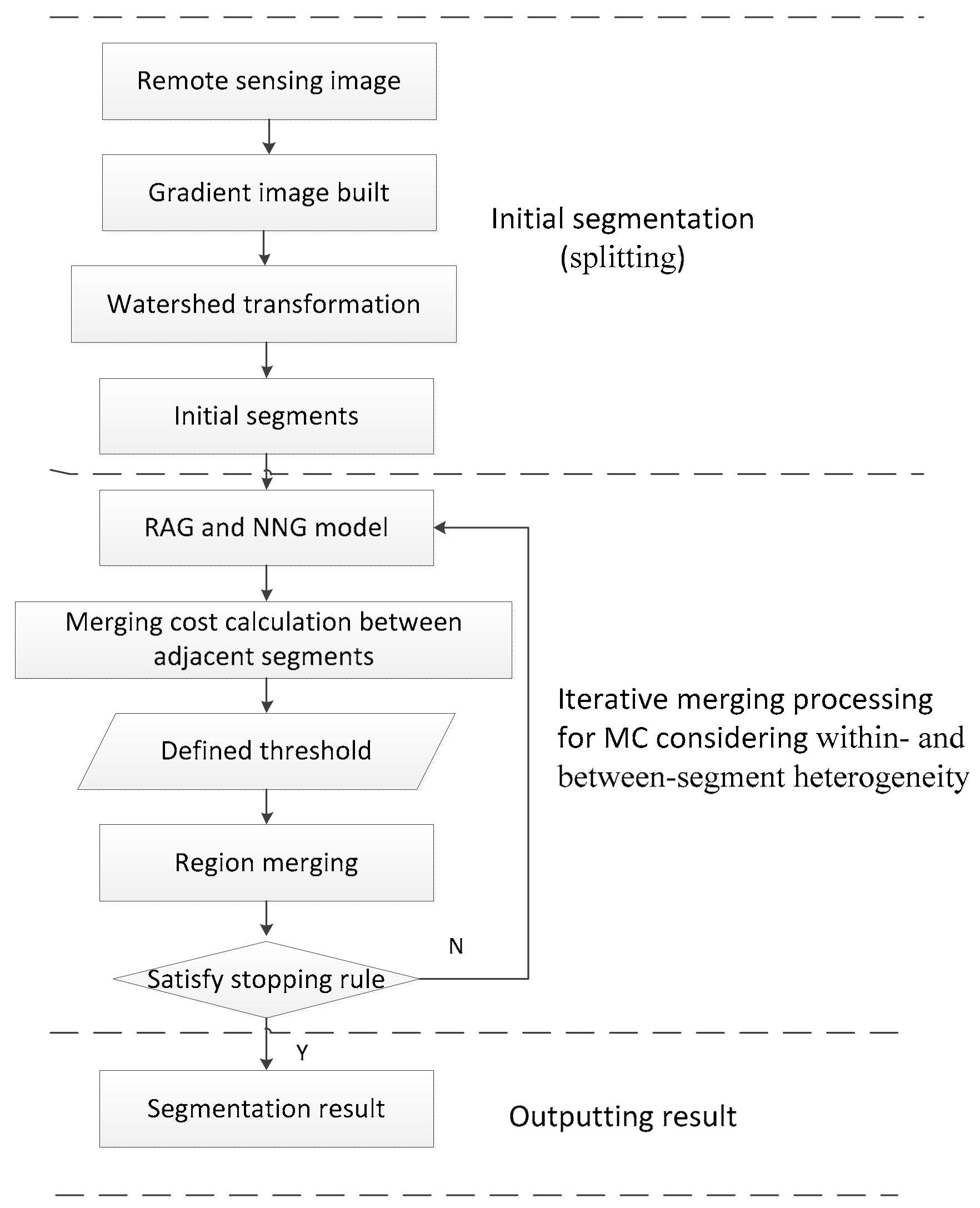
2.1. Overview
2.2. Watershed Transformation
2.3. Region Merging Based on Merging Criteria (MC) Considering Within- and Between-Segment Heterogeneity
2.3.1. MC Considering Within- and Between-Segment Heterogeneity
2.3.2. Region Merging Using the Objective Heterogeneity and Relative Homogeneity (OHRH) MC
2.4. Region Merging Based on MC Considering Between-Segment Heterogeneity
2.5. Segmentation Evaluation
3. Results
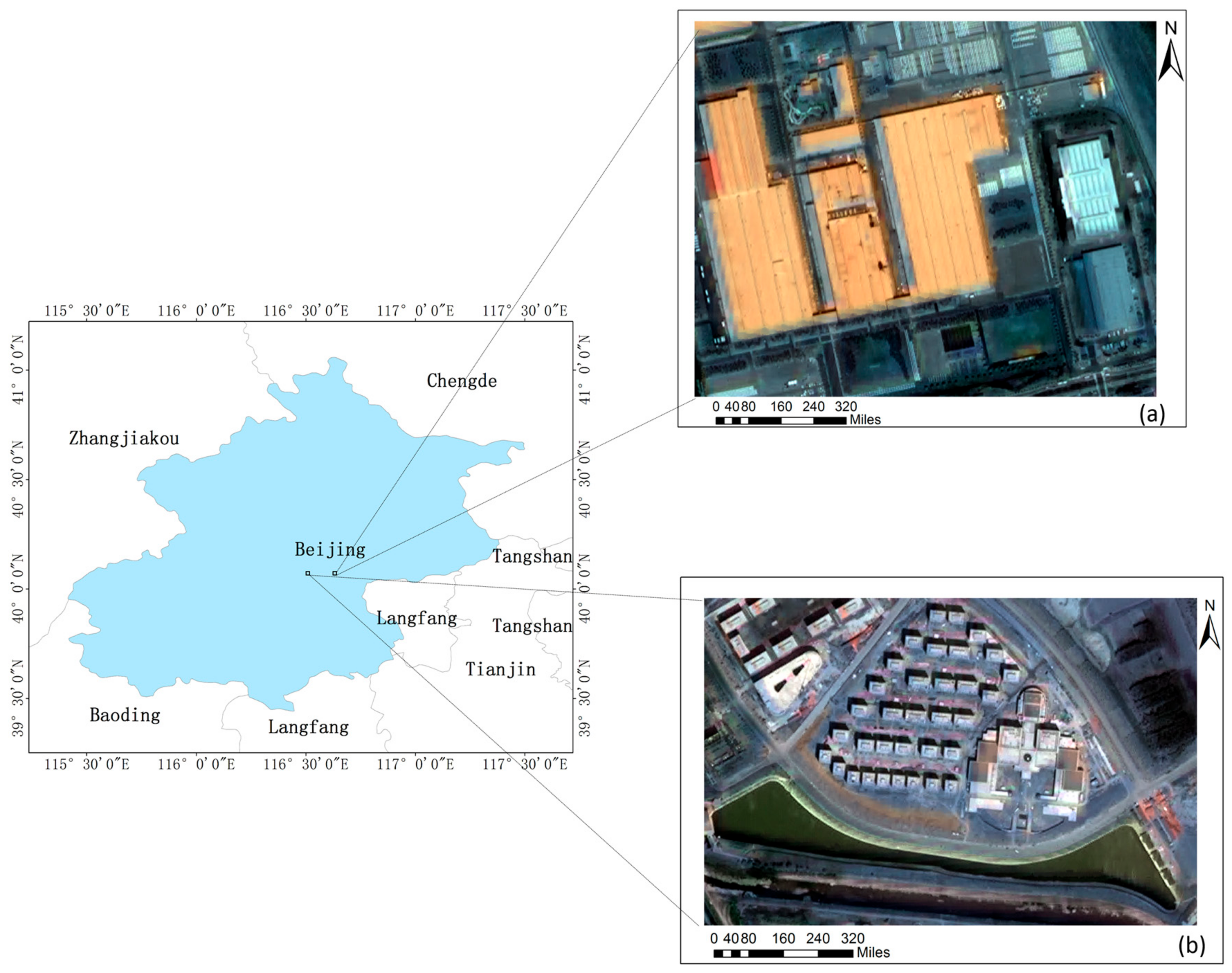
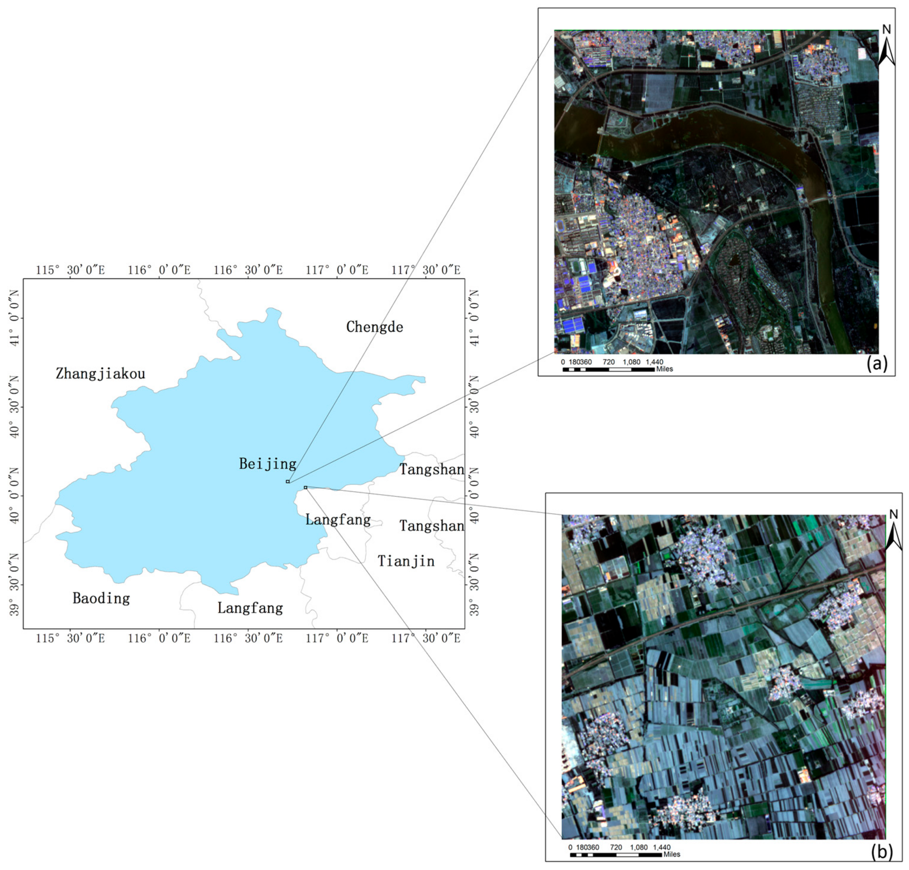
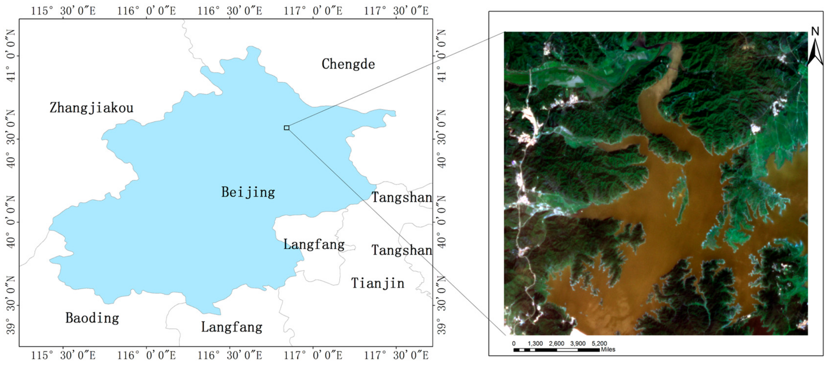
3.1. Study Area and Image
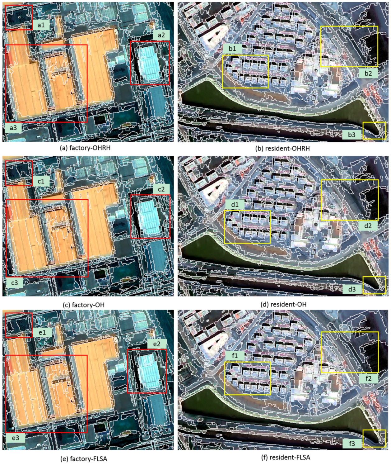
3.1.1. Urban Area
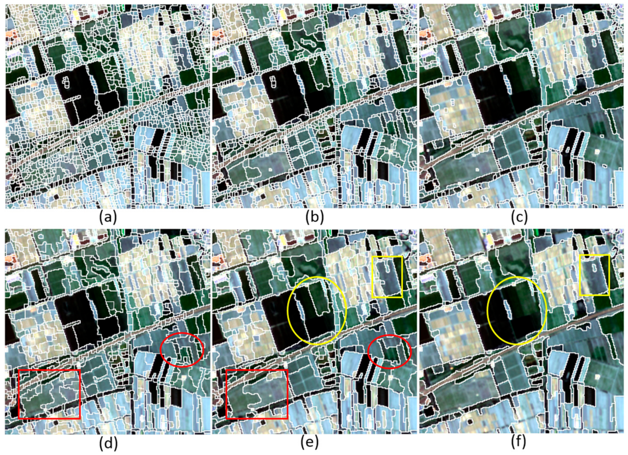
3.1.2. Rural Area
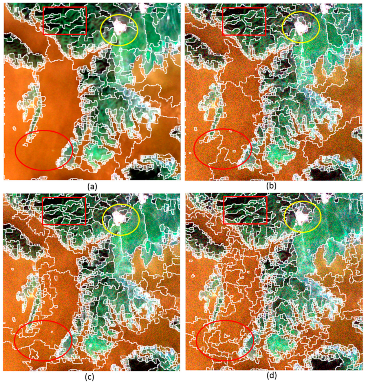
3.1.3. Forest Area
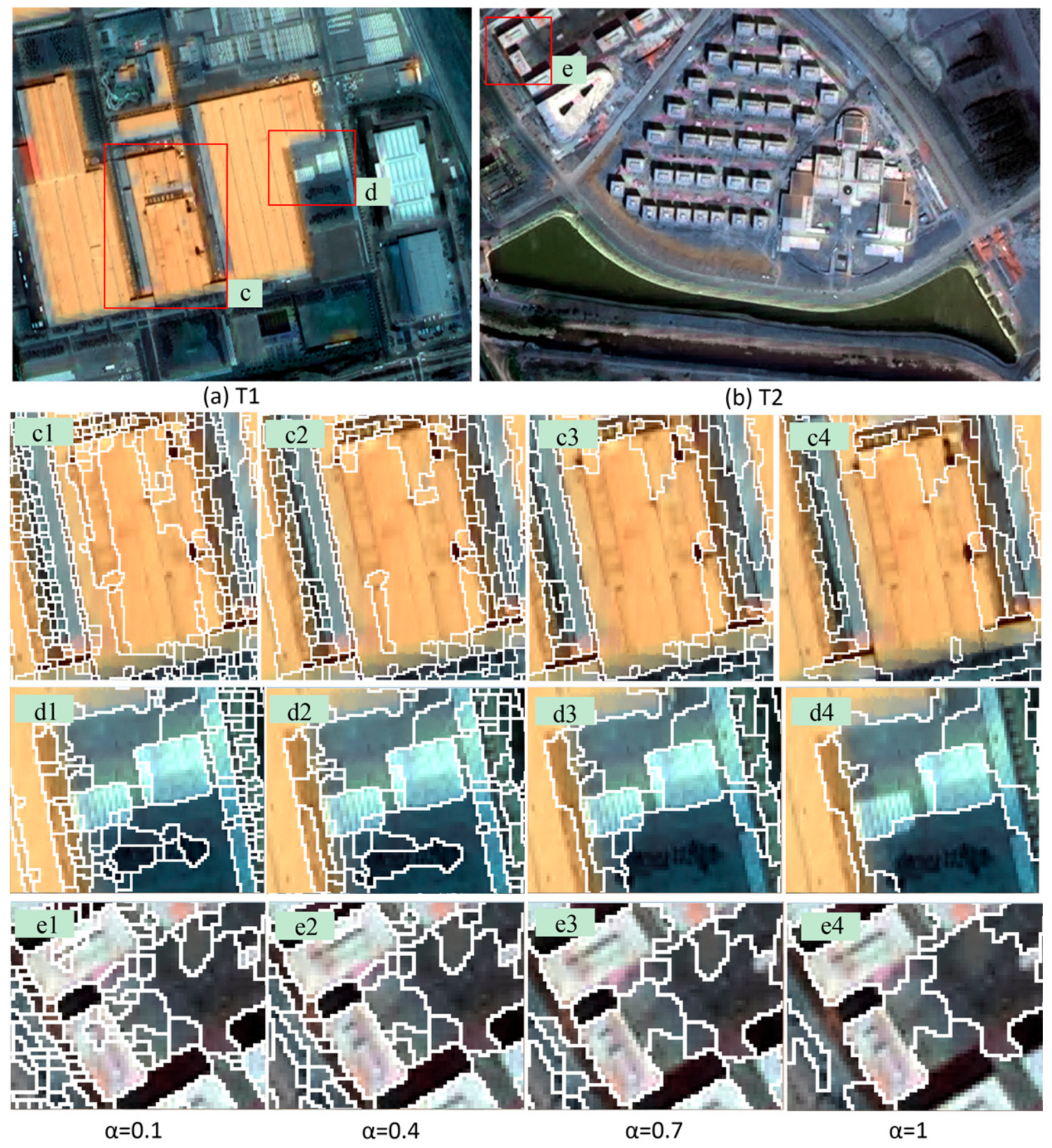
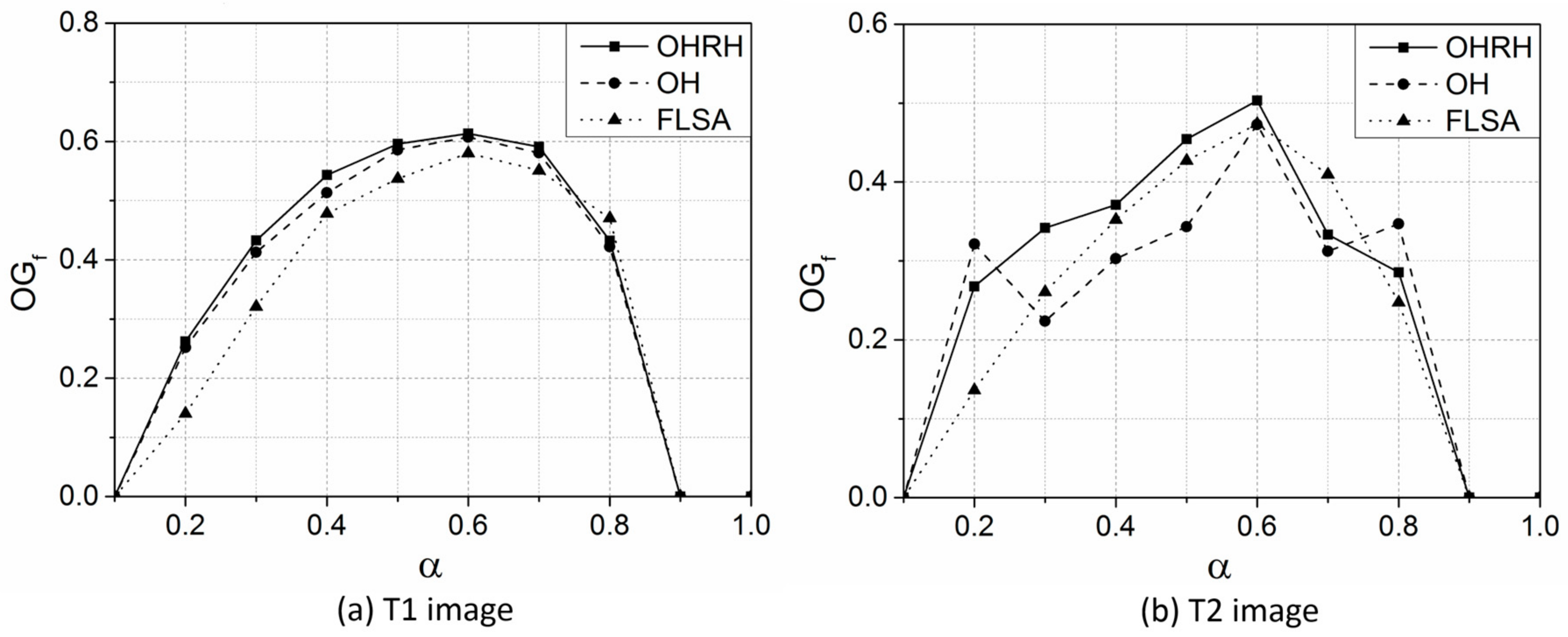
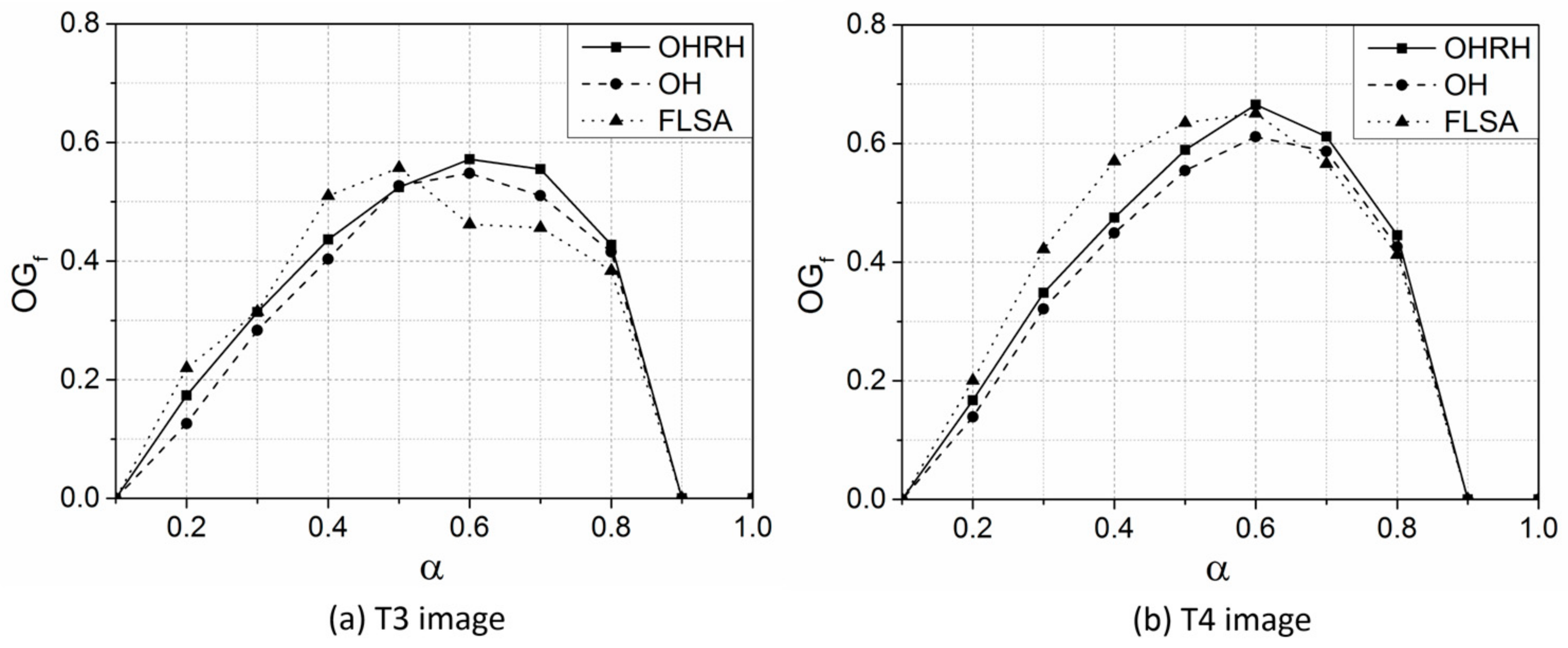
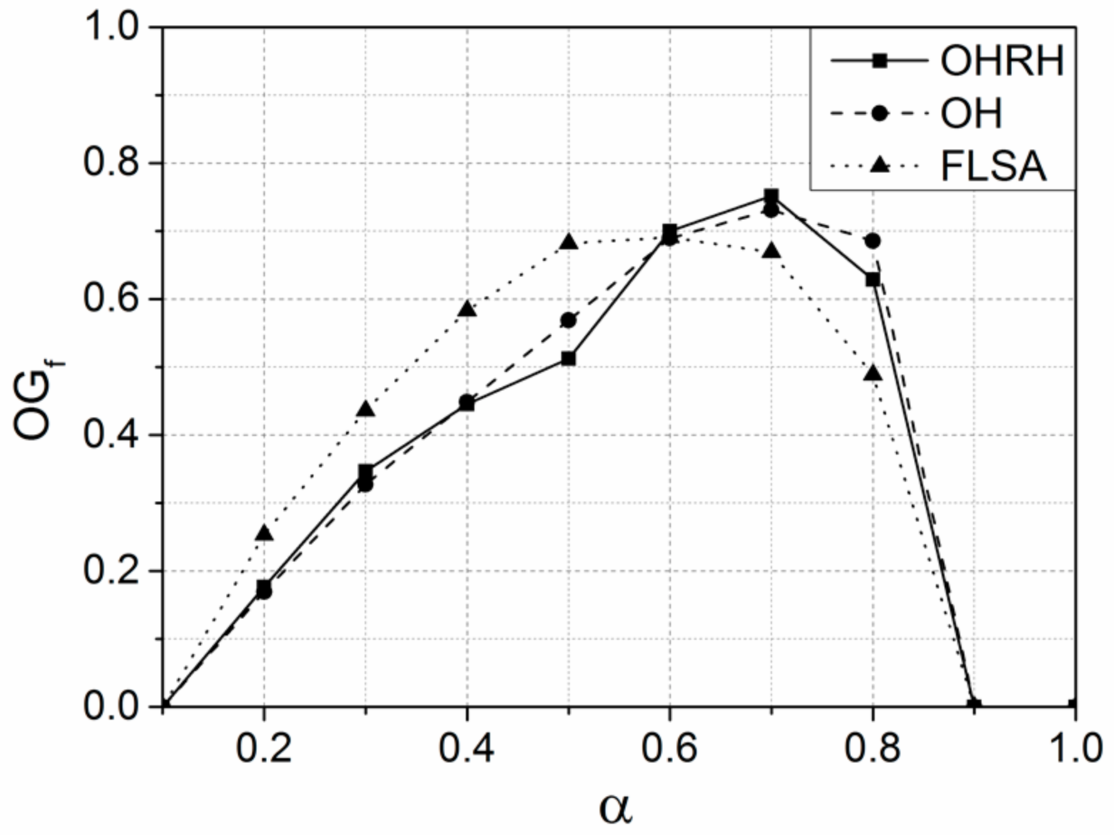
3.2. Sensitivity Analysis of the OHRH Method
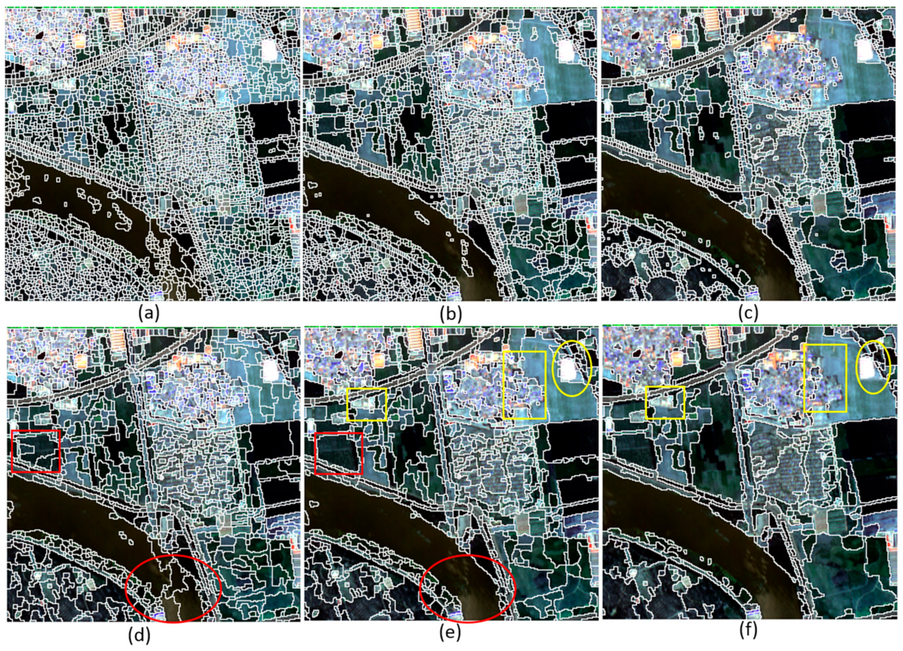
3.3. Comparative Analyses for the Three Region Merging Methods
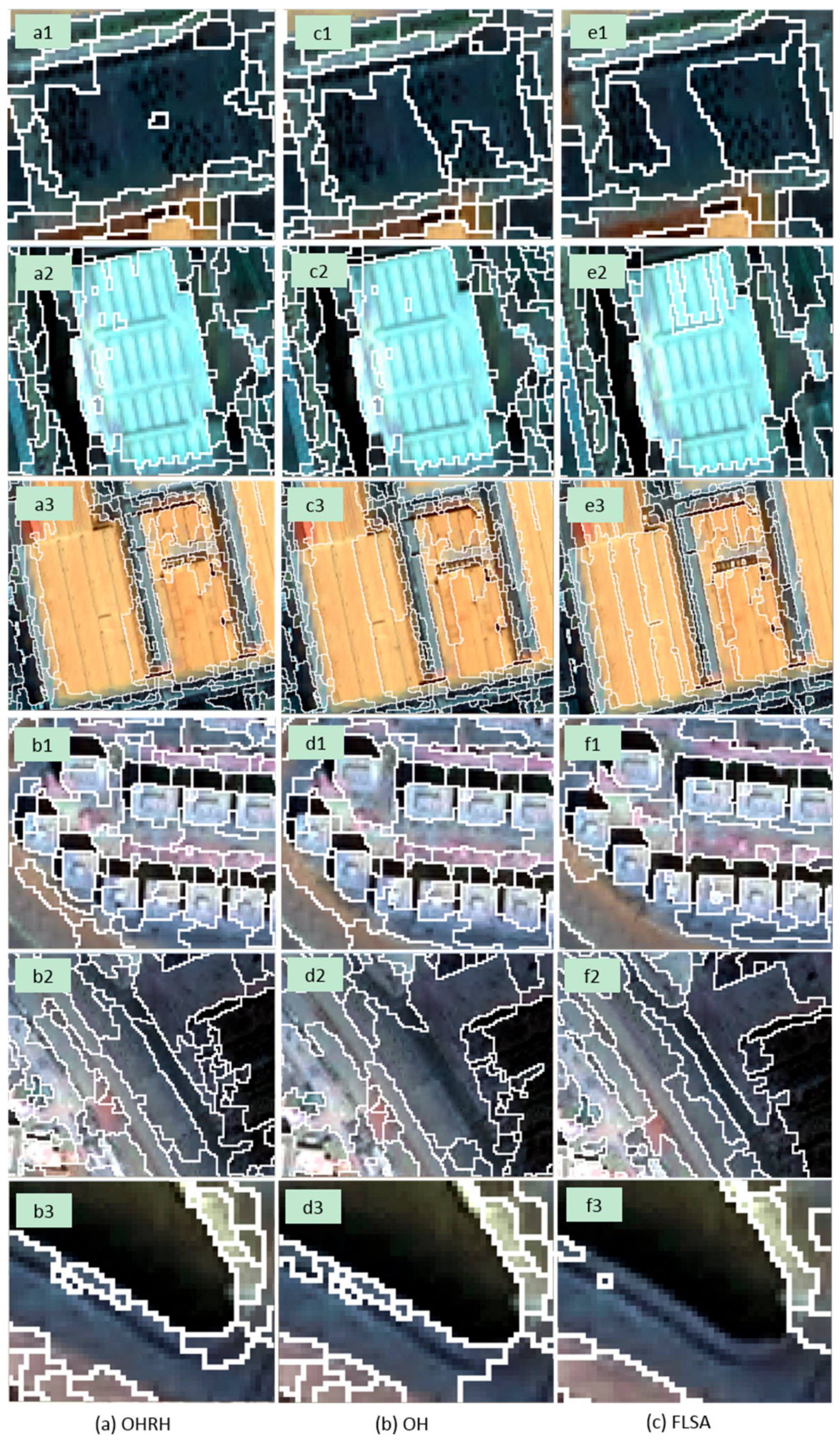
3.3.1. Urban Area
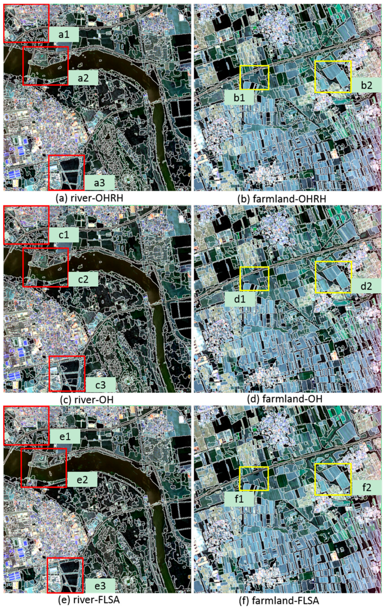
3.3.2. Rural Area
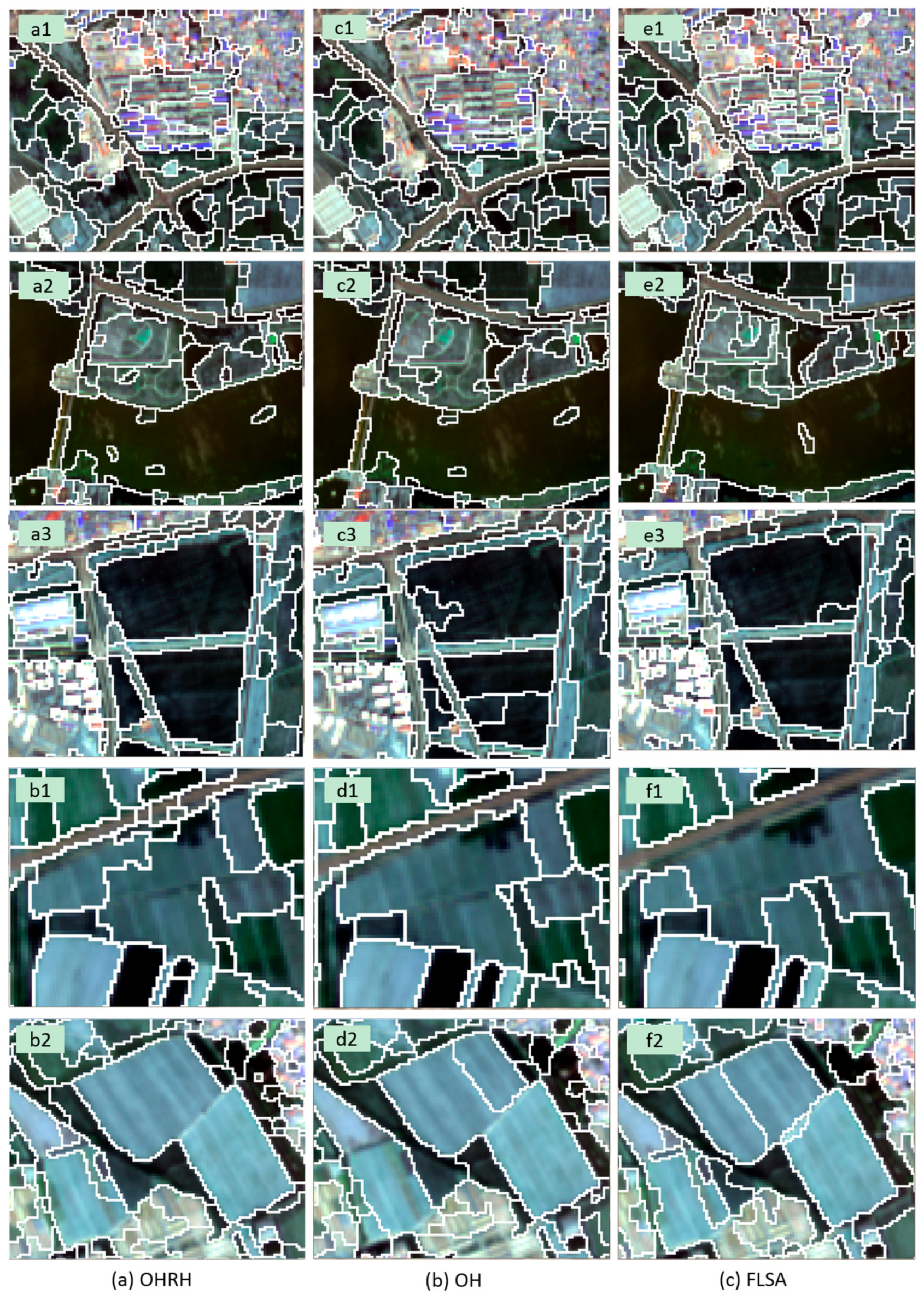
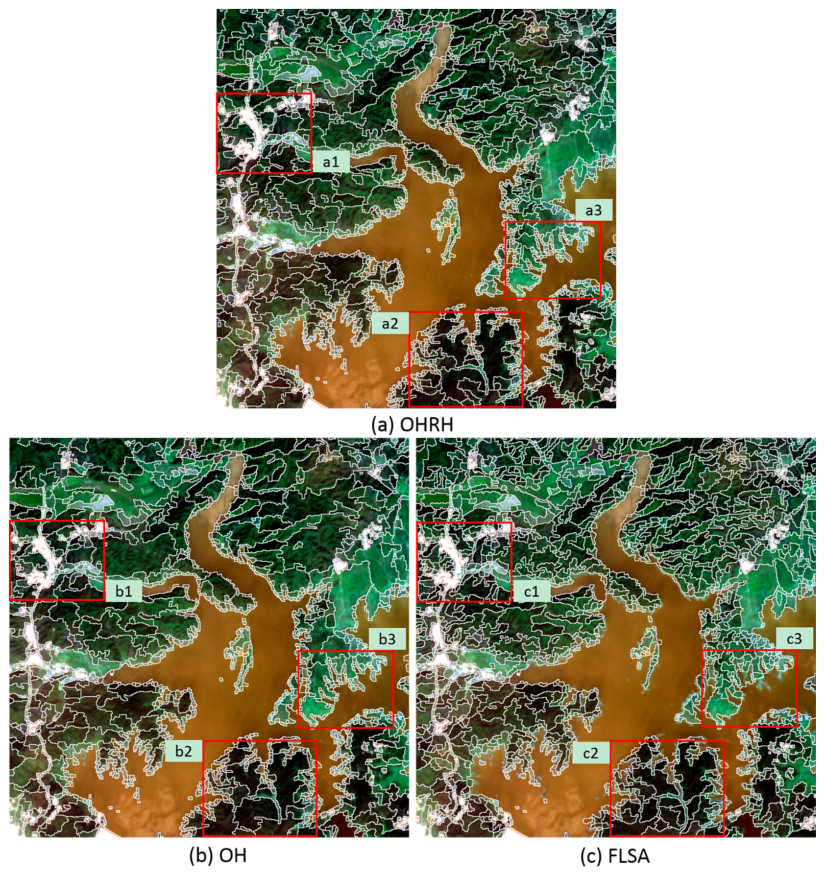
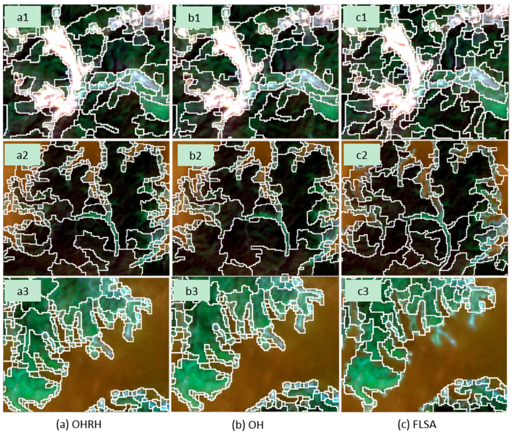
3.3.3. Forest Area
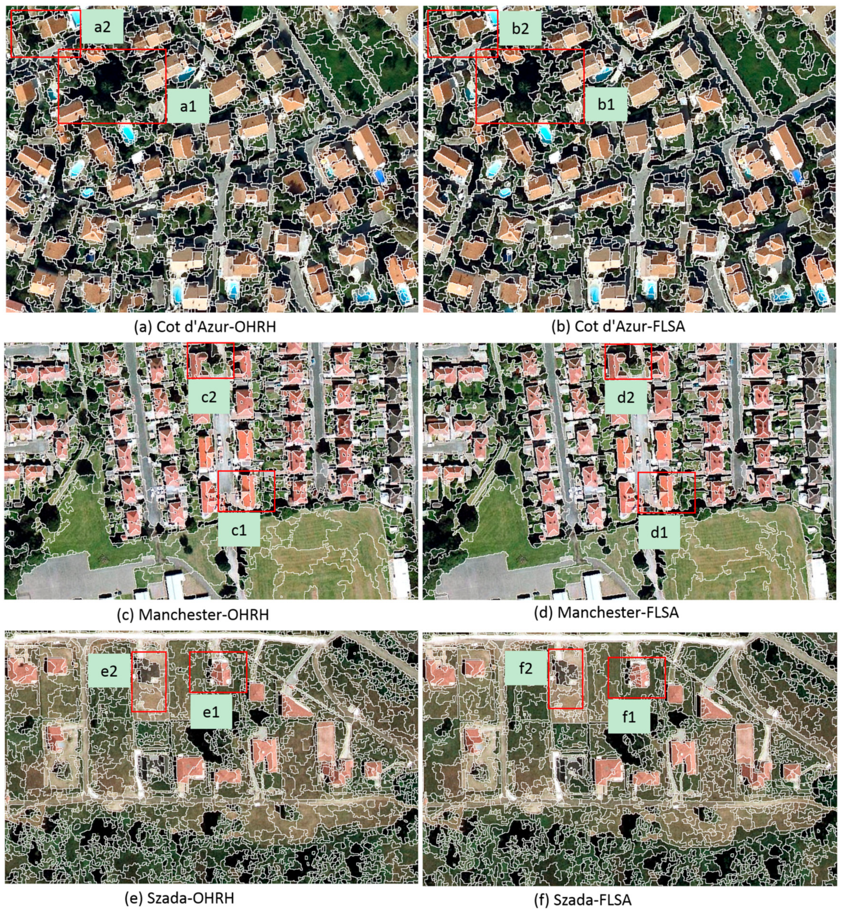
3.4. The Performance of the OHRH Method in Another Dataset
4. Discussion
5. Conclusions
Supplementary Materials
Author Contributions
Acknowledgments
Conflicts of Interest
References
- Blaschke, T. Object based image analysis for remote sensing. ISPRS J. Photogramm. 2010, 65, 2–16. [Google Scholar] [CrossRef]
- Blaschke, T.; Hay, G.J.; Kelly, M.; Lang, S.; Hofmann, P.; Addink, E.; Feitosa, R.Q.; van der Meer, F.; van der Werff, H.; van Coillie, F.; et al. Geographic object-based image analysis—Towards a new paradigm. ISPRS J. Photogramm. 2014, 87, 180–191. [Google Scholar] [CrossRef] [PubMed]
- Myint, S.W.; Gober, P.; Brazel, A.; Grossman-Clarke, S.; Weng, Q.H. Per-pixel vs. Object-based classification of urban land cover extraction using high spatial resolution imagery. Remote Sens. Environ. 2011, 115, 1145–1161. [Google Scholar] [CrossRef]
- Zhang, X.L.; Feng, X.Z.; Xiao, P.F.; He, G.J.; Zhu, L.J. Segmentation quality evaluation using region-based precision and recall measures for remote sensing images. ISPRS J. Photogramm. 2015, 102, 73–84. [Google Scholar] [CrossRef]
- Zhang, X.L.; Xiao, P.F.; Feng, X.Z.; Wang, J.G.; Wang, Z. Hybrid region merging method for segmentation of high-resolution remote sensing images. ISPRS J. Photogramm. 2014, 98, 19–28. [Google Scholar] [CrossRef]
- Hay, G.J.; Castilla, G.; Wulder, M.A.; Ruiz, J.R. An automated object-based approach for the multiscale image segmentation of forest scenes. Int. J. Appl. Earth Obs. 2005, 7, 339–359. [Google Scholar] [CrossRef]
- Johansen, K.; Arroyo, L.A.; Phinn, S.; Witte, C. Comparison of geo-object based and pixel-based change detection of riparian environments using high spatial resolution multi-spectral imagery. Photogramm. Eng. Remote Sens. 2010, 76, 123–136. [Google Scholar] [CrossRef]
- Liu, J.; Li, P.J.; Wang, X. A new segmentation method for very high resolution imagery using spectral and morphological information. ISPRS J. Photogramm. 2015, 101, 145–162. [Google Scholar] [CrossRef]
- Yang, J.; He, Y.H.; Caspersen, J.; Jones, T. A discrepancy measure for segmentation evaluation from the perspective of object recognition. ISPRS J. Photogramm. 2015, 101, 186–192. [Google Scholar] [CrossRef]
- Benz, U.C.; Hofmann, P.; Willhauck, G.; Lingenfelder, I.; Heynen, M. Multi-resolution, object-oriented fuzzy analysis of remote sensing data for GIS-ready information. ISPRS J. Photogramm. 2004, 58, 239–258. [Google Scholar] [CrossRef]
- Schiewe, J. Segmentation of high-resolution remotely sensed data-concepts, applications and problems. Int. Arch. Photogramm. Remote Sens. Spat. Inf. Sci. 2002, 4, 380–385. [Google Scholar]
- Zhou, Y.N.; Li, J.; Feng, L.; Zhang, X.; Hu, X.D. Adaptive scale selection for multiscale segmentation of satellite images. IEEE J.-Stars 2017, 10, 3641–3651. [Google Scholar] [CrossRef]
- Li, Y.; Cui, C.; Liu, Z.X.; Liu, B.X.; Xu, J.; Zhu, X.Y.; Hou, Y.C. Detection and monitoring of oil spills using moderate/high-resolution remote sensing images. Arch. Environ. Contam. Toxicol. 2017, 73, 154–169. [Google Scholar] [CrossRef] [PubMed]
- Li, Z.W.; Shen, H.F.; Li, H.F.; Xia, G.S.; Gamba, P.; Zhang, L.P. Multi-feature combined cloud and cloud shadow detection in gaofen-1 wide field of view imagery. Remote Sens. Environ. 2017, 191, 342–358. [Google Scholar] [CrossRef]
- Du, H.; Li, M.G.; Meng, J.A. Study of fluid edge detection and tracking method in glass flume based on image processing technology. Adv. Eng. Softw. 2017, 112, 117–123. [Google Scholar] [CrossRef]
- Tan, K.; Zhang, Y.; Tong, X. Cloud extraction from Chinese high resolution satellite imagery by probabilistic latent semantic analysis and object-based machine learning. Remote Sens. 2016, 8, 963. [Google Scholar] [CrossRef]
- Du, S.H.; Guo, Z.; Wang, W.Y.; Guo, L.; Nie, J. A comparative study of the segmentation of weighted aggregation and multiresolution segmentation. GISci. Remote Sens. 2016, 53, 651–670. [Google Scholar] [CrossRef]
- Grinias, I.; Panagiotakis, C.; Tziritas, G. Mrf-based segmentation and unsupervised classification for building and road detection in peri-urban areas of high-resolution satellite images. ISPRS J. Photogramm. 2016, 122, 145–166. [Google Scholar] [CrossRef]
- Zhao, H.H.; Xiao, P.F.; Feng, X.Z. Optimal gabor filter-based edge detection of high spatial resolution remotely sensed images. J. Appl. Remote Sens. 2017, 11, 015019. [Google Scholar] [CrossRef]
- Canny, J. A computational approach to edge-detection. IEEE Trans. Pattern Anal. 1986, 8, 679–698. [Google Scholar] [CrossRef]
- Comaniciu, D.; Meer, P. Mean shift: A robust approach toward feature space analysis. IEEE Trans. Pattern Anal. 2002, 24, 603–619. [Google Scholar] [CrossRef]
- Cheng, H.D.; Jiang, X.H.; Sun, Y.; Wang, J.L. Color image segmentation: Advances and prospects. Pattern Recogn. 2001, 34, 2259–2281. [Google Scholar] [CrossRef]
- Hong, T.H.; Rosenfeld, A. Compact region extraction using weighted pixel linking in a pyramid. IEEE Trans. Pattern Anal. 1984, 6, 222–229. [Google Scholar] [CrossRef]
- Leonardis, A.; Gupta, A.; Bajcsy, R. Segmentation of range images as the search for geometric parametric models. Int. J. Comput. Vis. 1995, 14, 253–277. [Google Scholar] [CrossRef]
- Zhu, S.C.; Yuille, A. Region competition: Unifying snakes, region growing, and bayes/mdl for multiband image segmentation. IEEE Trans. Pattern Anal. 1996, 18, 884–900. [Google Scholar]
- Khelifi, L.; Mignotte, M. Efa-bmfm: A multi-criteria framework for the fusion of colour image segmentation. Inform. Fusion 2017, 38, 104–121. [Google Scholar] [CrossRef]
- Su, T.F. A novel region-merging approach guided by priority for high resolution image segmentation. Remote Sens. Lett. 2017, 8, 771–780. [Google Scholar] [CrossRef]
- Zhou, C.B.; Wu, D.M.; Qin, W.H.; Liu, C.C. An efficient two-stage region merging method for interactive image segmentation. Comput. Electr. Eng. 2016, 54, 220–229. [Google Scholar] [CrossRef]
- Yang, J.; He, Y.H.; Caspersen, J. Region merging using local spectral angle thresholds: A more accurate method for hybrid segmentation of remote sensing images. Remote Sens. Environ. 2017, 190, 137–148. [Google Scholar] [CrossRef]
- Wang, M.; Li, R.X. Segmentation of high spatial resolution remote sensing imagery based on hard-boundary constraint and two-stage merging. IEEE Trans. Geosci. Remote 2014, 52, 5712–5725. [Google Scholar] [CrossRef]
- Canovas-Garcia, F.; Alonso-Sarria, F. A local approach to optimize the scale parameter in multiresolution segmentation for multispectral imagery. Geocarto Int. 2015, 30, 937–961. [Google Scholar] [CrossRef]
- Chen, J.; Deng, M.; Mei, X.M.; Chen, T.Q.; Shao, Q.B.; Hong, L. Optimal segmentation of a high-resolution remote-sensing image guided by area and boundary. Int. J. Remote Sens. 2014, 35, 6914–6939. [Google Scholar] [CrossRef]
- Johnson, B.; Xie, Z.X. Unsupervised image segmentation evaluation and refinement using a multi-scale approach. ISPRS J. Photogramm. 2011, 66, 473–483. [Google Scholar] [CrossRef]
- Robinson, D.J.; Redding, N.J.; Crisp, D.J. Implementation of a Fast Algorithm for Segmenting SAR Imagery; DSTO-TR-1242; Defence Science Technology Organisation: Fairbairn, Australia, 2002.
- Jin, X. Segmentation-Based Image Processing System. U.S. Patent 8,260,048, 4 September 2012. [Google Scholar]
- Chen, B.; Qiu, F.; Wu, B.F.; Du, H.Y. Image segmentation based on constrained spectral variance difference and edge penalty. Remote Sens. 2015, 7, 5980–6004. [Google Scholar] [CrossRef]
- Johnson, B.A.; Bragais, M.; Endo, I.; Magcale-Macandog, D.B.; Macandog, P.B.M. Image segmentation parameter optimization considering within- and between-segment heterogeneity at multiple scale levels: Test case for mapping residential areas using landsat imagery. ISPRS Int. J. Geo-Inf. 2015, 4, 2292–2305. [Google Scholar] [CrossRef]
- Yang, J.; He, Y.H.; Weng, Q.H. An automated method to parameterize segmentation scale by enhancing intrasegment homogeneity and intersegment heterogeneity. IEEE Geosci. Remote Sens. 2015, 12, 1282–1286. [Google Scholar] [CrossRef]
- Yang, J.; Li, P.J.; He, Y.H. A multi-band approach to unsupervised scale parameter selection for multi-scale image segmentation. ISPRS J. Photogramm. 2014, 94, 13–24. [Google Scholar] [CrossRef]
- Tremeau, A.; Colantoni, P. Regions adjacency graph applied to color image segmentation. IEEE Trans. Image Proc. 2000, 9, 735–744. [Google Scholar] [CrossRef] [PubMed]
- Cheng, B.; Yang, J.C.; Yan, S.C.; Fu, Y.; Huang, T.S. Learning with l(1)-graph for image analysis. IEEE Trans. Image Proc. 2010, 19, 858–866. [Google Scholar] [CrossRef] [PubMed]
- Haris, K.; Efstratiadis, S.N.; Maglaveras, N.; Katsaggelos, A.K. Hybrid image segmentation using watersheds and fast region merging. IEEE Trans. Image Proc. 1998, 7, 1684–1699. [Google Scholar] [CrossRef] [PubMed]
- Vincent, L.; Soille, P. Watersheds in digital spaces–an efficient algorithm based on immersion simulations. IEEE Trans. Pattern Anal. 1991, 13, 583–598. [Google Scholar] [CrossRef]
- Roerdink, J.B.T.M.; Meijster, A. The watershed transform: Definitions, algorithms, and parallelization strategies. Fundam. Inform. 2001, 41, 187–228. [Google Scholar]
- Wagner, B.; Dinges, A.; Muller, P.; Haase, G. Parallel volume image segmentation with watershed transformation. Lect. Notes Comput. Sci. 2009, 5575, 420–429. [Google Scholar]
- Piretzidis, D.; Sideris, M.G. Adaptive filtering of goce-derived gravity gradients of the disturbing potential in the context of the space-wise approach. J. Geodesy 2017, 91, 1069–1086. [Google Scholar] [CrossRef]
- Sun, Y.; He, G.J. Segmentation of high-resolution remote sensing image based on marker-based watershed algorithm. In Proceedings of the Fifth International Conference on Fuzzy Systems and Knowledge Discovery, Jinan, China, 18–20 October 2008; pp. 271–276. [Google Scholar]
- Liu, L.M.; Wen, X.F.; Gonzalez, A.; Tan, D.B.; Du, J.; Liang, Y.T.; Li, W.; Fan, D.K.; Sun, K.M.; Dong, P.; et al. An object-oriented daytime land-fog-detection approach based on the mean-shift and full lambda-schedule algorithms using eos/modis data. Int. J. Remote Sens. 2011, 32, 4769–4785. [Google Scholar] [CrossRef]
- Espindola, G.M.; Camara, G.; Reis, I.A.; Bins, L.S.; Monteiro, A.M. Parameter selection for region-growing image segmentation algorithms using spatial autocorrelation. Int. J. Remote Sens. 2006, 27, 3035–3040. [Google Scholar] [CrossRef]
- Mikelbank, B.A. Quantitative geography: Perspectives on spatial data analysis, by A. S. Fotheringham, C. Brunsdon, and M. Charlton. Geogr. Anal. 2001, 33, 370–372. [Google Scholar] [CrossRef]
- Xiao, L.; Wang, R.L.; Dai, B.; Fang, Y.Q.; Liu, D.X.; Wu, T. Hybrid conditional random field based camera-lidar fusion for road detection. Inf. Sci. 2018, 432, 543–558. [Google Scholar] [CrossRef]
- Iabchoon, S.; Wongsai, S.; Chankon, K. Mapping urban impervious surface using object-based image analysis with worldview-3 satellite imagery. J. Appl. Remote Sens. 2017, 11. [Google Scholar] [CrossRef]
- Benedek, C.; Descombes, X.; Zerubia, J. Building development monitoring in multitemporal remotely sensed image pairs with stochastic birth-death dynamics. IEEE Trans. Pattern Anal. 2012, 34, 33–50. [Google Scholar] [CrossRef] [PubMed] [Green Version]


| Input: Output: | Remote-Sensing Image, Preliminary Segments Obtained from Watershed Transformation, and α Final Segmentation Result |
|---|---|
| Step 1: | Create a region-adjacent graph (RAG) and nearest neighbor graph (NNG) and calculate the merging cost between each adjacent segment by Equation (7) |
| Step 2: | Calculate the merging value T by Equation (8), and then select the adjacent segments for which the merging cost (t(s1,s2)) is the lowest, and merge them if t(s1,s2) ≤ T |
| Step 3: | Repeating step 1 and step 2, the iterative process is stopped when t(s1,s2) > T ( must only be calculated once) |
| Step 4: | Output the final segmentation result |
| Image | OGf | |
|---|---|---|
| OHRH | FLSA | |
| Côte d’Azur | 0.5864 | 0.5902 |
| Manchester | 0.5151 | 0.5012 |
| Szada | 0.6983 | 0.6794 |
© 2018 by the authors. Licensee MDPI, Basel, Switzerland. This article is an open access article distributed under the terms and conditions of the Creative Commons Attribution (CC BY) license (http://creativecommons.org/licenses/by/4.0/).
Share and Cite
Wang, Y.; Meng, Q.; Qi, Q.; Yang, J.; Liu, Y. Region Merging Considering Within- and Between-Segment Heterogeneity: An Improved Hybrid Remote-Sensing Image Segmentation Method. Remote Sens. 2018, 10, 781. https://doi.org/10.3390/rs10050781
Wang Y, Meng Q, Qi Q, Yang J, Liu Y. Region Merging Considering Within- and Between-Segment Heterogeneity: An Improved Hybrid Remote-Sensing Image Segmentation Method. Remote Sensing. 2018; 10(5):781. https://doi.org/10.3390/rs10050781
Chicago/Turabian StyleWang, Yongji, Qingyan Meng, Qingwen Qi, Jian Yang, and Ying Liu. 2018. "Region Merging Considering Within- and Between-Segment Heterogeneity: An Improved Hybrid Remote-Sensing Image Segmentation Method" Remote Sensing 10, no. 5: 781. https://doi.org/10.3390/rs10050781