Remote Sensing of Coastal Upwelling in the South-Eastern Baltic Sea: Statistical Properties and Implications for the Coastal Environment

Abstract

A detailed study of wind-induced coastal upwelling (CU) in the south-eastern Baltic Sea is presented based on an analysis of multi-mission satellite data. Analysis of moderate resolution imaging spectroradiometer (MODIS) sea surface temperature (SST) maps acquired between April and September of 2000–2015 allowed for the identification of 69 CU events. The Ekman-based upwelling index (UI) was applied to evaluate the effectiveness of the satellite measurements for upwelling detection. It was found that satellite data enable the identification of 87% of UI-based upwelling events during May–August, hence, serving as an effective tool for CU detection in the Baltic Sea under relatively cloud-free summer conditions. It was also shown that upwelling-induced SST drops, and its spatial properties are larger than previously registered. During extreme upwelling events, an SST drop might reach 14 °C, covering a total area of nearly 16,000 km². The evolution of an upwelling front during such intensive events is accompanied by the generation of transverse filaments extending up to 70 km offshore. An analysis of the satellite optical data shows a clear decline in the chlorophyll-a concentration in the coastal zone and in the shallow Curonian Lagoon, where it drops down by an order of magnitude. It was also shown that a cold upwelling front alters the stratification in the atmospheric boundary layer, leading to a sudden drop of air temperature and near-surface winds.

1. Introduction

Coastal upwelling (CU), a phenomenon found in large stratified lakes, estuaries, and oceans [1], is an important process for ecologically sensitive regions of the global ocean, such as the Baltic Sea, a large brackish water body that has a very limited water exchange with the open ocean through the narrow and shallow Danish straits [2]. Its extensive coastlines oriented in many directions also mean that coastal upwelling can occur with sustained wind over the Baltic Sea in almost any direction [3], which makes upwelling quite a common process [4].

Coastal upwelling is one of the main factors affecting the circulation and the ecosystem of the Baltic Sea region. It is responsible for the mixing of water masses [5] as well as for water exchange between the coastal zone and the open sea; the formation of frontal zones with strong cross-front property gradients [6,7]; and the modification of biotic and abiotic conditions of marine ecosystems by bringing cold, nutrient rich waters from the depth to the euphotic layer [8]. The formation of upwelling fronts also importantly modifies the vertical stratification and turbulent regime in the marine–atmosphere boundary layer (MABL), resulting in a change in the surface wind stress and direction in the coastal zone [3,9].

Nutrient-rich waters brought up from deeper layers to the surface, particularly in the summer time, and the exposure of upwelled phytoplankton to surface radiation enhances the primary production and phytoplankton biomass during upwelling events [10,11], hence influencing the coastal pelagic communities and higher trophic levels [12]. Moreover, upwelling-related coastal ocean dynamics may eventually modify the spatial patterns of background algae blooms in the coastal zone by transporting them farther offshore.

During the summer-time holiday season, CU might also have a negative impact on particular tourist areas as a result of a rapid drop in water and air temperatures near the shore [2]. Furthermore, bathing tourism depends on good water quality, while post-upwelling phytoplankton blooms might significantly reduce it, making coastal waters unattractive for recreation [13].

The need to study coastal upwelling in the Baltic Sea is also essential in order to assess the regional variability of water and energy exchange, salinity dynamics, and the response of marine ecosystems to extreme events—some of the “Grand Challenges” of the Baltic Earth Science Plan [14], established in 2016. Thus, the upwelling phenomenon is indeed of certain interest to researchers, fishermen, and coastal managers [15]. The availability of wide spatial and temporal coverage multi-spectral satellite data comes in handy when gathering information on coastal upwelling properties, as conventional in situ monitoring methods are limited in space to resolve the full spatial patterns of upwelling properties, its dynamics, and implications to the coastal environment. Besides, the size and complexity of coastal waters makes it difficult to monitor them with ships and buoys alone, while satellites are proving to be cost-effective for observing large ocean and coastal areas [16]. Our study is primarily based on the utilization of satellite infrared and visible band data, which is now traditionally used for such studies (e.g., [1,9,17,18]), and has certain advantages over in situ measurements and models in that it provides the spatial details and dynamical features of the phenomena.

In general, Baltic Sea coastal upwelling has received considerable attention in the literature (e.g., [2,19,20,21]). In this work, our focus is on the south-eastern (SE) part of the Baltic Sea, a frequent location of upwelling development under northerly winds (see e.g., [2,4,19]). Yet, no comprehensive investigations of upwelling properties have been carried out so far in this region; most of the existing works have typically addressed CU across the entire Baltic Sea basin, providing limited information about its development and implications for the SE Baltic (SEB). Several model studies analyzed the upwelling generation and evolution process, and its vertical structure in the study region; however, their results appear to underestimate the horizontal upwelling parameters when compared to satellite-derived sea surface temperature (SST) maps [22,23,24]. More details about the fine horizontal structure of CU front in the SEB are available from two case studies based on high-resolution synthetic aperture radar (SAR) measurements combined with infrared (IR) SST maps and models [9,17]. Yet, these works have very limited temporal coverage and considered only a few upwelling events, and primarily addressed the mechanisms of upwelling manifestation in the satellite data.

Our aim here is to provide the first detailed record of coastal upwelling events and their statistical properties in the SE Baltic Sea during 16 years of satellite observations, from 2000–2015, with a special focus on a major upwelling event in the summer of 2006. As will be further shown, coastal upwelling has a significant influence on the environmental conditions not only of the SE Baltic Sea, but also in the shallow Curonian Lagoon. In Section 2, the data and methods are addressed, while the main results of the satellite-based analysis and discussion follow in Section 3. Section 4 contains a summary followed by conclusions.

2. Materials and Methods

2.1. Satellite Data

In this work, we used Terra/Aqua Moderate Resolution Imaging Spectroradiometer (MODIS) SST maps for the period 2000–2015 to characterize SE Baltic Sea coastal upwelling from the distribution and evolution of its surface thermal signatures. MODIS Level 2 daytime (MODIS thermal bands 31 (11 μ) and 32 (12 μ) images (L2_LAC_SST product)) covering the study site with a spatial resolution of about 1 km [25] were obtained from the NASA OceanColor website [26]. The validation of this product against in situ observations in the SE Baltic and the Curonian Lagoon carried out by the authors of [27] showed a very good correspondence between space-borne and conventional SST measurements, suggesting that MODIS-based SST retrievals can be further used to analyze SST development over the study region.

The MODIS SST images were processed using ESA BEAM and MathWorks © MATLAB software. A visual inspection was done to eliminate cloud-covered images. In total, about 1700 satellite images covering 16 years of observations between April and September were processed, from which 239 images were further used to analyze the statistical properties of CU in the SE Baltic Sea.

For the demonstration of the CU impact on the spatial distribution of the chlorophyll-a (chl-a) concentration in the coastal waters of the Baltic Sea during the major upwelling event in July 2006, a MERIS/Envisat (Medium Resolution Imaging Spectrometer onboard the Envisat satellite, European Space Agency) full resolution (300 m nadir) image acquired on 17 July was used. For the estimation of the chl-a concentration, a FUB processor (1.2.4 version, plug-in in BEAM/VISAT software) was applied, as described and validated in the literature [28]. This study showed a good agreement between the MERIS-derived and in situ measured chl-a with R² = 0.87, root mean square error (RMSE) = 14.44 mg m³ (N = 56).

Six MERIS/Envisat full resolution cloud free images acquired between 17 July–3 August 2006 were used to map the chl-a in the Curonian Lagoon. The chl-a concentration was estimated using a semi-empirical band ratio algorithm applied to the images after atmospheric correction with the Satellite Signal in the Solar Spectrum (6SV) code, as described and validated in the literature [29,30], and after revision in the literature [31]. The previous studies demonstrated a good agreement between the MERIS-derived and in situ measured chl-a in the Curonian Lagoon, with R² = 0.93.

To address the upwelling impact on the coastal wind conditions, high-resolution near-surface wind fields were derived from the corresponding Envisat Advanced SAR (ASAR) images acquired between 16 July and 19 July 2006, using the CMOD4 model function [32], and the wind direction from the NCEP GFS 0.5° six-hourly wind forecast.

2.2. In Situ Measurements

Three-hourly wind speed and direction data sampled at a height of 10 m at the Klaipeda coastal monitoring station, provided by the Lithuanian Hydrometeorological Service under the Ministry of Environment of the Republic of Lithuania, were used for the analysis of the upwelling-favorable meteorological conditions. The Klaipeda station was chosen as a representative point of wind conditions along the SE Baltic Sea coastline. The water temperature and salinity data from the Klaipeda, Nida, and Palanga hydrometeorological stations sampled 1–2 m from the coast in the upper 0.5 m of the water column, provided by the Department of Marine Research (Lithuanian Environmental Protection Agency), were used to trace the upwelling signatures in these records.

2.3. Satellite-Based Analysis of Upwelling Parameters

Following the methodology of previous research [20,33], a 2 °C threshold was used (temperature drop of ≥2 °C relative to the ambient waters) to identify the coastal upwelling events in the satellite SST images and to exclude other processes with temperature changes not associated with coastal upwelling (e.g., diurnal temperature changes, etc.).

The primary upwelling parameters derived from the analysis of the satellite data include the upwelling frequency and duration, upwelling-related SST drop, and cross-frontal horizontal SST gradient, as well as the main spatial parameters of the upwelling front—its cross-shore and alongshore extent, and the total area. The upwelling frequency was calculated as the number of upwelling events per single thermally-stratified period from April to September of any given year. The duration of a single upwelling event was calculated as the sum of the days that the upwelling signatures were detectable in the SST maps [1]. An upwelling-induced SST drop (∆T) was defined as the difference between the mean SST of the ambient (upwelling-free) waters and the minimum SST value over the particular transect across the upwelling front (Figure 1), while the total area of the upwelling-affected waters was calculated from the corresponding low-temperature pixels.

Horizontal SST gradient, SST drop, and the cross-shore extent of the upwelling front were retrieved from the SST data taken along eight transects that were normal to the SE Baltic Sea coast (shown in Figure 1). One transect is located next to the Sambian peninsula (denoted as Kaliningrad), three transects—along the Lithuanian coast (close to Nida, Klaipeda, and Palanga), and four along the Latvian coast (near Pape, Liepaja, Jurkalne, and Venstpils). As seen from Figure 1, the coastline of the study site is oriented so that northerly and north-easterly winds favor upwelling development. To evaluate the upwelling impact on the shallow hypereutrophic coastal lagoon, one transect was also located in the northern part of the Curonian Lagoon (Figure 1).

2.4. Ekman-Based Upwelling Index

The computations for deriving the upwelling indices were described by Bakun [34], and since then have been widely used to estimate the upwelling strength and seasonal variability, as well as for a better understanding of the physical–biological coupling [35,36,37,38].

As an additional tool for the identification of upwelling events in the observational data, we also used an upwelling index (UI), which allowed us to identify the number of upwelling events that could have evolved under the real wind conditions measured at the coastal stations. The UI represents a measure of the volume of water that upwells (positive values) or downwells (negative values) at the coast, owing to coastal divergence of geostrophic winds [35,36].

Following the authors of [37], the Ekman transport can be calculated in terms of wind speed at the 10 m level, W; seawater density, ρ_w = 1025 kg m⁻³; a dimensionless drag coefficient, $C_d=0.0012\left(0.066\left|W\right|+0.63\right)$ adapted for the Baltic Sea (according to [20]); and air density, ρ_a (assumed to be constant at 1.22 kg m⁻³), as follows:

$$Q_x=\frac{{\rho }_a{C}_d}{{\rho }_{w}f}{(W_x^2+W_y^2)}^{1/2}{W}_y$$

(1)

$$Q_y=-\frac{{\rho }_a{C}_d}{{\rho }_{w}f}{(W_x^2+W_y^2)}^{1/2}{W}_x$$

(2)

where f is the Coriolis parameter, defined as twice the vertical component of the Earth’s angular velocity, Ω, about the local vertical given by f = 2Ω sin (θ) at latitude θ. Finally, the subscript $x$ corresponds to the zonal component and the subscript $y$ to the meridional one. Then, UI can be defined as the Ekman transport component in the direction perpendicular to the shoreline, as follows:

$$\mathrm{UI}=Q\perp =-\sin \left(\mathsf{\theta }\right)Q_x+\cos \left(\mathsf{\theta }\right)Q_y$$

(3)

where θ = π/2 + φ, and φ is the angle of the unitary vector perpendicular to the shoreline pointing landward (at the Klaipeda station φ = 90°).

In this work, the calculations of UI were carried out using observational data from the Klaipeda station, as it has a central location over the study region. The time-span of the analysis was limited to the upwelling-favorable season, from April to September 2000–2015. To calculate the daily upwelling indices, three-hourly wind data were averaged daily to better fulfil the Ekman conditions, and later, the UI values were multiplied by a factor of 10³ to represent the displacement of volume for each kilometre of the coast (m³ s⁻¹ km⁻¹). The start and end of the upwelling favorable conditions were defined as the date when the daily mean upwelling index became positive (started to decrease). The cumulative upwelling index (CUI) (i.e., the sum of daily values before the start of each upwelling event when UI was positive) was calculated in order to better understand the response of upwelling to favorable meteorological conditions.

3. Results and Discussion

An analysis of the satellite SST images allowed for the identification of 69 distinct coastal upwelling events during the study period, from April to September 2000–2015. In this section, we first compared the satellite-based upwelling identification with the use of the upwelling index calculated from in situ measurements (Section 3.1), followed by an analysis of the upwelling-favorable meteorological conditions presented in Section 3.2. A detailed description of the main spatial and temporal parameters of coastal upwelling in the SEB, including the upwelling-induced modulation of SST, are given in Section 3.3. Section 3.4 describes the major upwelling event recorded in the summer of 2006, as well as its impact on the spatial properties of the chl-a distribution and near-surface wind field.

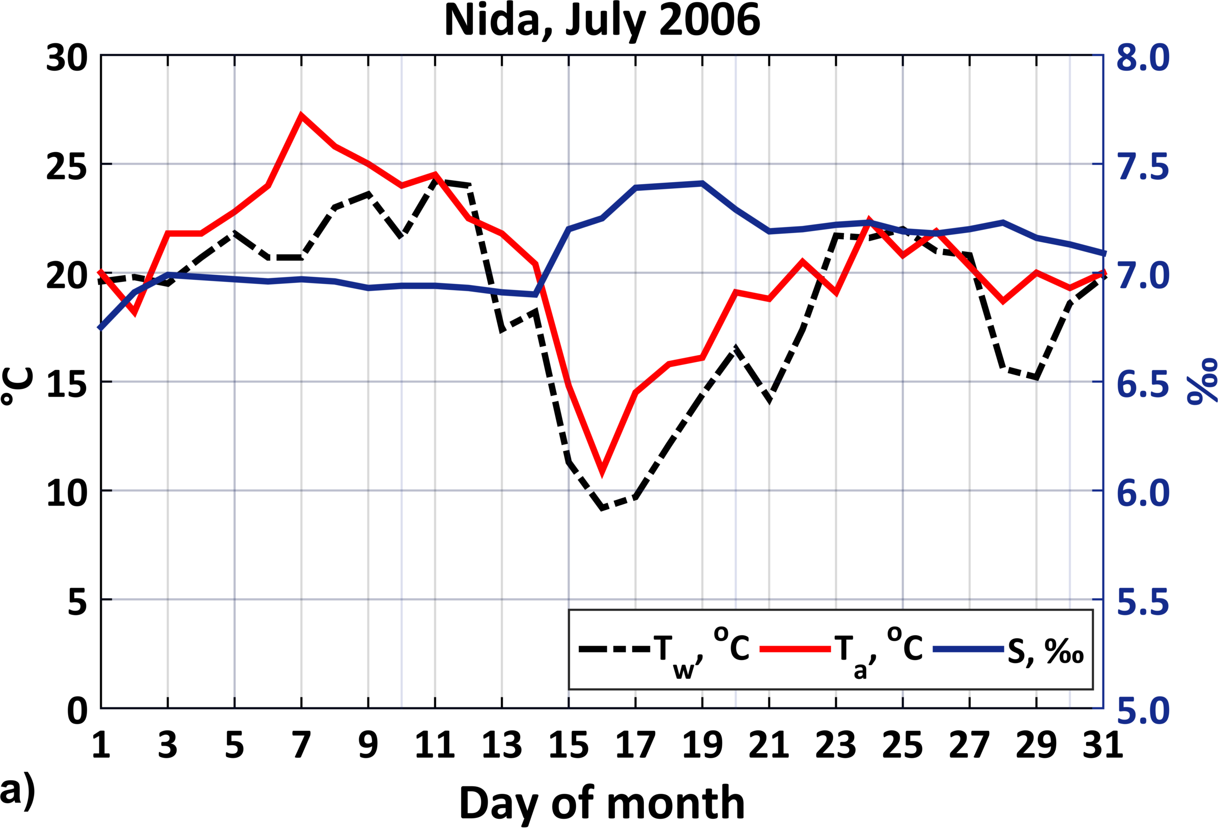
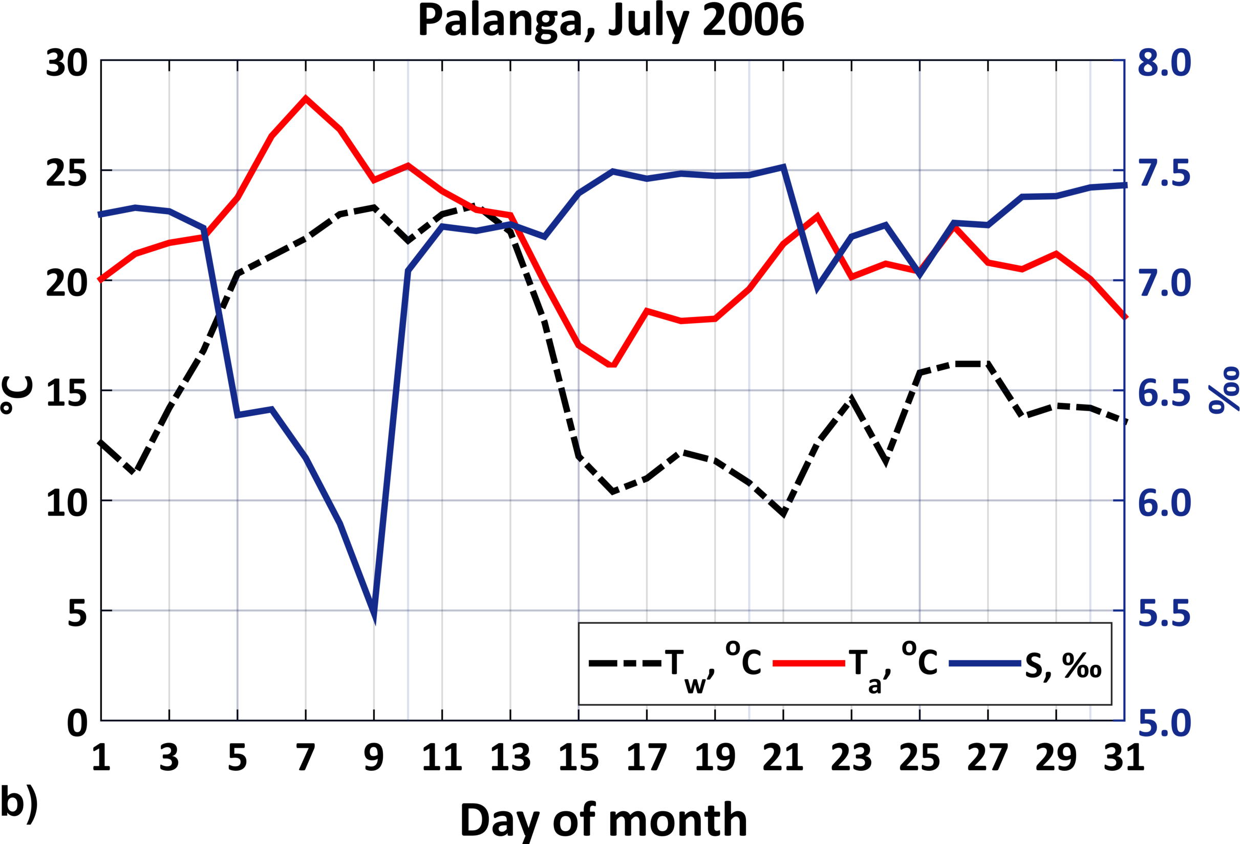
3.1. Satellite Observations vs. Coastal Measurements

To evaluate the effectiveness of the satellite infrared (IR) SST measurements for upwelling detection in the SE Baltic Sea, we analyzed the daily water temperature (T_w) records and upwelling index values calculated from in situ wind measurements, and compared them to our satellite-based statistics. According to the authors of [39], it usually takes about 60 h of mild, permanent direction winds to cause upwelling in the Baltic Sea. We therefore considered positive UI values observed for several days in a row and formed under northerly winds as the conditions eligible for upwelling formation. The evaluation of UI enabled the identification of 96 upwelling events, meaning that satellite-based results represent about 72% of the total of all possible UI-based events. As Figure 2 shows, the largest discrepancies between these two are found in April and September. In April, this might be attributed to the fact that the background water temperature is relatively low during this month, $\overline{T}=6$°C (see, e.g., Figure 4 in the literature [27]), and, hence, the SST contrast between the ambient and upwelled waters is not well pronounced in the satellite data. A possible reason for missing CU events in September might be a deepening of the mixed layer as a result of the thermal convection and turbulent mixing during autumn [40], making it difficult to distinguish low intensity upwelling events in IR SST data. The last and most important reason is a relatively small number of cloud-free satellite data during these months (see Figure 2). In turn, the analysis of satellite data enables us to observe 87% of the upwelling events identified with UI during the May–August period, implying that the satellite IR imagery is a rather effective tool for upwelling studies in the SE Baltic Sea under relatively cloud-free summer conditions.

As some existing coastal upwelling studies rely only on direct water temperature records made at coastal stations (see, e.g., [41]), this might eventually result in some upwelling events being missed. As further shown in Figure 2, the use of water temperature measurements from coastal stations allowed for the identification of only 58 upwelling events, which is 40% less than the number of theoretical events and about 15% less than those detected in the satellite data.

Furthermore, the analysis of in situ T_w measurements from the coastal monitoring stations enabled the authors of [41] to identify only 20 upwelling events along the Lithuanian coast during the summer periods of 1993–2011 (i.e., significantly fewer than in our study during a shorter time period). The reason behind such a small number of upwelling detections in the coastal T_w records might be a possible location of an upwelling front at some distance from the coast. Moreover, even in cases when upwelling is clearly recorded in the direct measurements, an upwelling-associated temperature drop will be underestimated anyway, as the cold upwelling core lies some distance from the coast. This is well exemplified in the SST profiles shown in Figure 3, where, depending on the season, the first few pixels near the coast usually have higher SST values and do not represent upwelling core temperatures, especially in the locations where the bottom slope is not very steep. For example, near Pape, where the slope is not as steep as it is near Klaipeda and Nida, the cold upwelling core might be as far as 3–8 km from the coast. The largest difference of 2–3 °C between the near-coast and the upwelling-core SST values is observed across all of the stations in spring and summer, while in autumn, this effect is almost negligible. One may conclude that the satellite data are indeed efficient tools for observing and quantifying the upwelling parameters, as the coastal T_w records might miss some upwelling events or underestimate the upwelling-associated water temperature drop. Even though conventional measurements and theoretical calculations are effective under cloud cover, they are not able to provide any information on the spatial properties of the upwelling front described below.

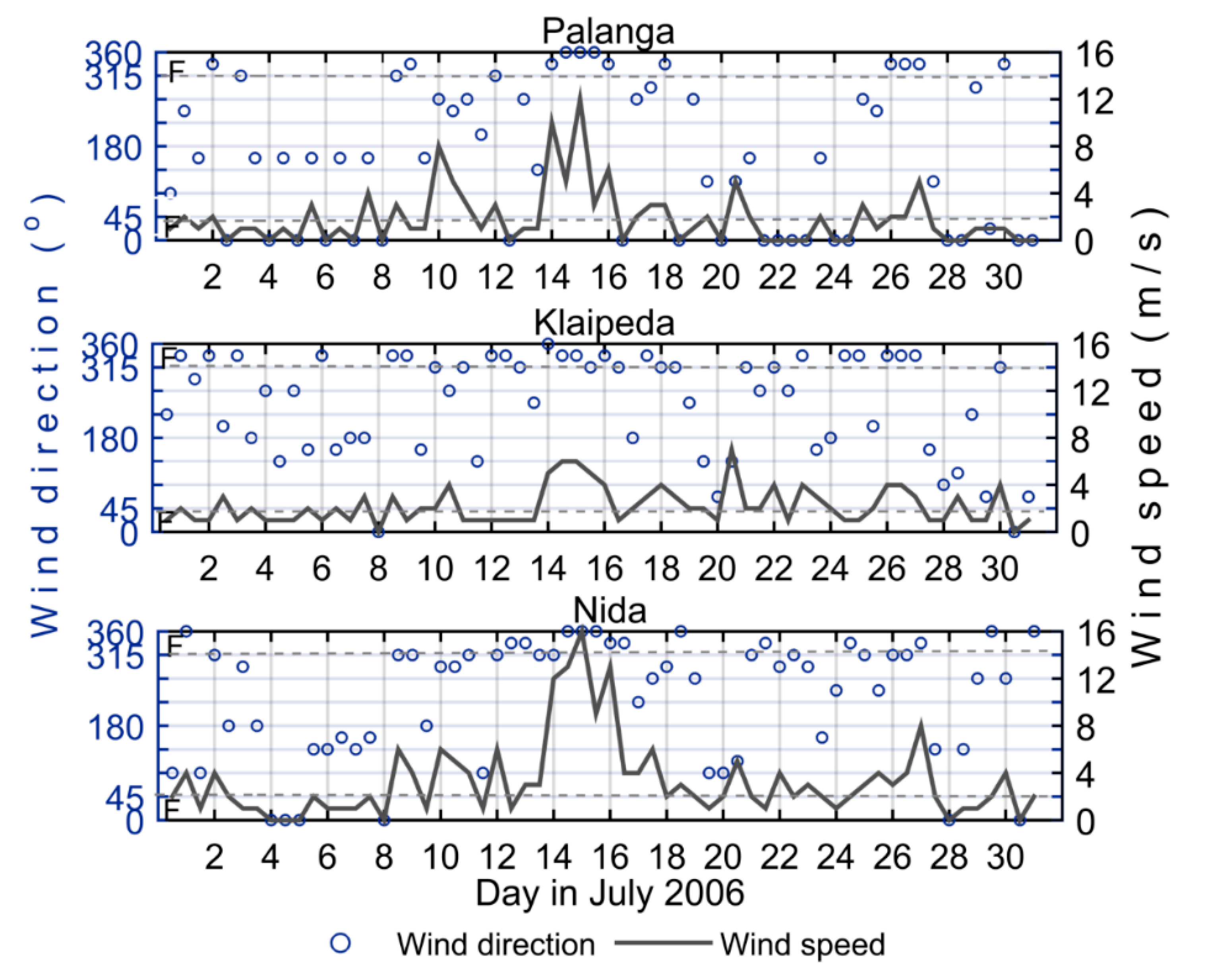
3.2. Meteorological Conditions Prior to Upwelling Development

In general, wind conditions in the Baltic Sea region are dominated by westerlies [42] with south-westerly (SW), northerly (N), and north-easterly (NE) winds occurring most frequently over the entire Baltic Sea basin [43]. However, upwelling events are rather episodic here [44], varying in accordance with the local winds and coastline configuration. The N and NE winds are known to trigger coastal upwelling in the SE Baltic Sea, and in only in the northernmost part of Latvia and along the Polish coast it is favored by winds from other directions.

Some monthly patterns of upwelling-favorable winds might be seen in the coastal records (Figure 4), providing useful information on the phenology of coastal upwelling phenomena over the study site. Figure 4 shows the monthly wind roses for April–September 2000–2015, built from the wind field data taken at the Klaipeda station. As seen, westerly winds clearly prevailed during the warm period. In turn, upwelling-favorable northerly winds were more pronounced during the spring months, with N–NE winds comprising 21% in April and 18% in May. In June and July, the recurrence of northerly winds decreased to about 15–17%, rising again to about 20% in August and September. In general, upwelling-favorable winds are usually mild, not exceeding 9 m s⁻¹, and it was only in April that a small portion of stronger winds of 9–12 m s⁻¹ was observed.

Furthermore, to analyze the upwelling response to the meteorological conditions, an upwelling index and cumulative upwelling index (CUI) are used. Figure 5a shows that in ~23% of the events, the upwelling system might respond quite rapidly, and the first surface signatures of cold upwelled waters appear just one day after positive UI values start to be recorded. Yet, more generally, about 1–3 days of positive UI values are needed for the upwelling front to be manifested in SST data, in agreement with the literature [39]. In about 35% of cases, usually observed in April and September (Figure 5c), the upwelling signatures are manifested only four or more days after the favorable wind conditions have been established. As seen in Figure 5b, the CUI values prior to the upwelling development range from 50 to 900 m³ s⁻¹ km⁻¹. More than half (63%) have values of up to 200 m³ s⁻¹ km⁻¹, and only 9% are much larger, in the range of 600–900 m³ s⁻¹ km⁻¹.

Figure 5c shows the intra-seasonal variation of the CUI and the number of days with positive UI before the upwelling manifestation in the satellite data. As seen, both parameters have a clear seasonal pattern—milder upwelling-favorable winds with a shorter duration are required to generate an upwelling event during the summer months when the seasonal thermocline is shallow and the vertical stratification of the water column is at its strongest, and a longer and stronger wind impulse is needed in the spring and in early autumn. It takes only about 2.5 days with an average CUI of 150–220 m³ s⁻¹ km⁻¹ to cause the upwelling in June and July, and more persistent yet weaker winds in August (Figure 5c). In late spring and early autumn, the positive UI values should last one–two days longer (3.5–4.5 days) with CUI values near 300 m³ s⁻¹ km⁻¹, implying that more wind energy is needed to trigger the upwelling over the less stratified water column [39].

3.3. Statistical Parameters of Coastal Upwelling in the SE Baltic Sea

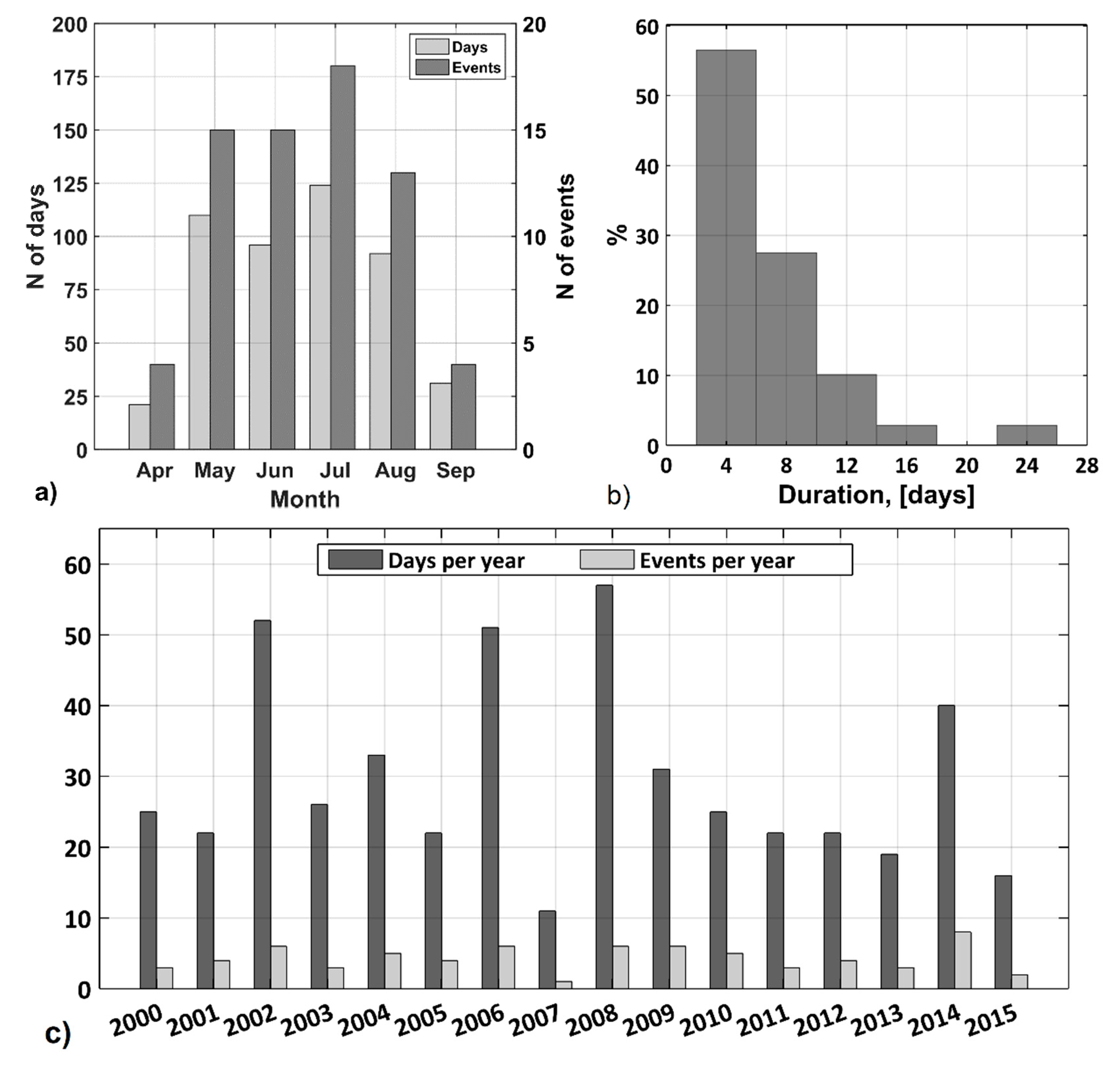
3.3.1. Upwelling Season, Frequency, and Duration

Figure 6a shows the monthly distribution of the total number of upwelling events and the number of days with upwelling identified over the entire study period. In general, upwelling events were detected during the thermally stratified season between April and September, with the earliest registered on 14 April 2010 and the latest on 23 September 2008. About 90% of the events were observed between May and August, with a clear peak in July, when 18 events were registered. As expected, July is also characterized by the maximum number of upwelling days (124 days) during 2000–2015, equal to eight upwelling days per month on average. For the high upwelling season (from May to August), the monthly averaged value is about seven upwelling days per month, or 20–25% of the month.

It is interesting to note, that although the N and NE winds and associated Ekman transport were rather strong in April and September (Figure 4 and Figure 5c), the number of identified upwelling events is low during these months, which is perhaps related to the weak vertical stratification in April and the wind-induced deepening of the mixed layer in September.

Figure 6b shows a histogram distribution of the upwelling duration. As seen, short-lived upwelling events that are two–six days long clearly dominate (57% of the total number), while about 27% of the events persisted for seven–ten days. Yet, in some distinct cases, the coastal upwelling may last up to 23 days, as observed in summer 2006 and 2008, and may result from the chain of consecutive upwelling events. In such a case, the first upwelling event may contribute significantly to the formation of the initial stratification setup for the next one, when the relatively weak winds can lead to upwelling [45]. While not so frequent, such long-lasting events might be of great importance for the whole region, influencing both the natural (e.g., weather, ecosystems) and socio-economic (e.g., tourism) environment of the coastal area.

The frequency of coastal upwelling ranged from one (in 2007) to several events per thermally stratified period, occurring about four times per season on average (Figure 6c). The highest number of upwelling events was recorded in 2014 (eight events), but these were rather short, covering only about 20% of the warm period. The longest upwelling seasons were recorded in 2002, 2006, and 2008, with six upwelling events each year lasting for 52, 51, and 57 days, respectively, covering about 30% of the warm period.

The authors of [21] analyzed the upwelling frequencies for different Baltic Sea regions based on the visual analysis of the satellite SST data from May to September 1990–2009. They found the highest upwelling frequencies (up to 25%) along the Swedish coast in the western Gotland Basin and in the Bornholm Basin. Frequencies of 10–15% were found along the western Finish and Estonian coast, while the SE Baltic coast had a range of frequency of 5–12%. In our study, the season mean number of upwelling days accounted for about 16% of the warm season (~30 days), that is, somewhat longer than reported by the authors of [21] and [24], who recorded 27 upwelling days from the re-analysis data for 1970–2010 in this part of the Baltic Sea. Our results also show that the CU in the SE Baltic Sea is more frequent than, for example, along the nearby Polish coast, with 23 upwelling days (13% of the warm period from April to September), as recorded in the literature [46].

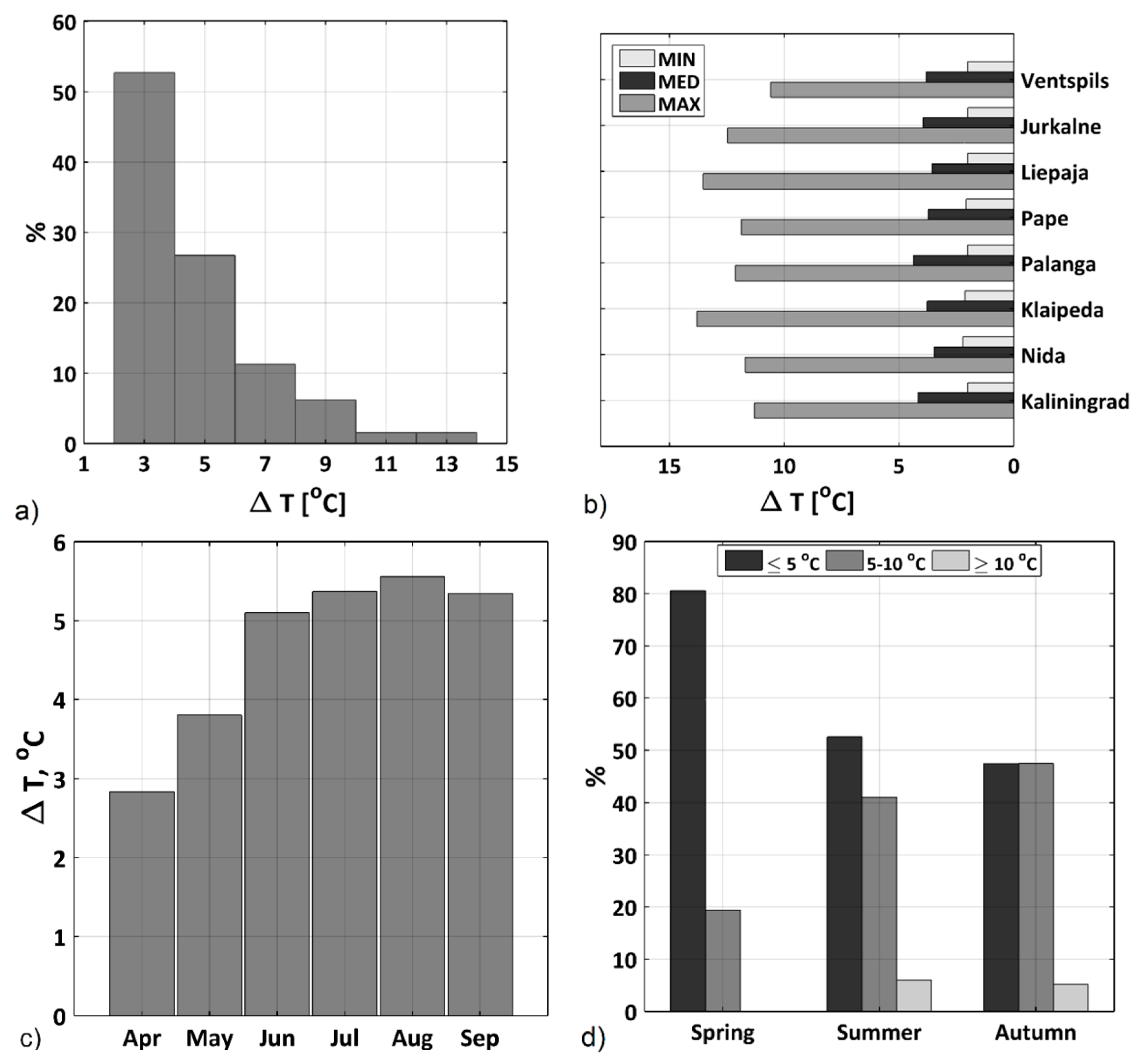
3.3.2. Modulation of Sea Surface Temperature

One of the key changes induced by coastal upwelling in the marine environment is a rapid drop of sea surface temperature, which might strongly influence the coastal ecosystems through the direct effects of temperature on species performance, and indirectly through species interactions [47]. In order to evaluate the modulation of the sea surface temperature during coastal upwelling events, we defined it in terms of the SST drop (∆T) and the horizontal SST gradient calculated from the SST values taken along eight cross-frontal transects, as shown in Figure 1.

According to the authors of [41], the temperature drop during the upwelling events near the Lithuanian and Latvian coasts is about 4–8 °C. A similar range of ∆T values is observed in our records, but the maximal values can reach up to 10–14 °C (Figure 7a). As Figure 7b shows, there are no significant latitudinal differences in ∆T values along the SEB coast, with maximum and median values of about 12 °C and 4 °C, respectively. At the same time, one can clearly see a distinct seasonal variability of ∆T, shown in Figure 7c,d. For instance, the average value of the SST drop is around 3.5 °C in spring, while in summer and autumn, when the surface layer is already warmed up, it is ~5.3 °C (Figure 7c). The number of ∆T values of 5–10 °C gradually rise from spring to autumn, while the highest SST drop values (>10 °C) are more frequently observed in the summer than in autumn (Figure 7d).

The typical values of the SST gradient across the upwelling front range between 0.2 and 0.5 °C km⁻¹ (Figure 8a). In 25% of cases, they are larger than 0.6 °C km⁻¹, with maximum recorded values of about 1.6 °C km⁻¹. These values are somewhat lower than those given in the literature [4], and they agree with the results presented by the authors of [19,48].

Moreover, considerable spatial variations of the SST gradient are evident (Figure 8b). As seen, the strength of the local SST gradient changes and depends on the width of the upwelling zone over a particular location (Figure 8b), even though the upwelling-associated SST drop is nearly similar along the SEB coast (Figure 7b). Higher values of the SST gradient are observed across relatively narrow parts of the upwelling front near Ventspils, Palanga, and Klaipeda, where the maximum (median) values of the SST gradient are about 1.5 °C km⁻¹ (0.5 °C km⁻¹). Moderate SST gradients were observed near Pape, Nida, and Kaliningrad, while the lowest values were found near Jurkalne and Liepaja, where the upwelling zone is widest (see Figure 9 and Figure 10).

Furthermore, the seasonal variations of the SST gradients are also visible (Figure 8c,d). In spring, weak (<0.25 °C km⁻¹) SST gradients are dominant (in about 52% of the cases), while in summer and autumn, SST gradients that are higher than 0.25 °C km⁻¹ clearly prevail (58% in summer, 63% in autumn). The highest values (>0.75 °C km⁻¹) are observed more frequently in the summer than in spring or autumn. Accordingly, the lowest monthly mean SST gradients are recorded in April (0.21 °C km⁻¹), and gradually become higher throughout the warm season, with a clear peak in July (0.43 °C km⁻¹). Starting from August, a decreasing tendency is observed towards autumn, with a monthly mean SST gradient of 0.36 °C km⁻¹ observed in September.

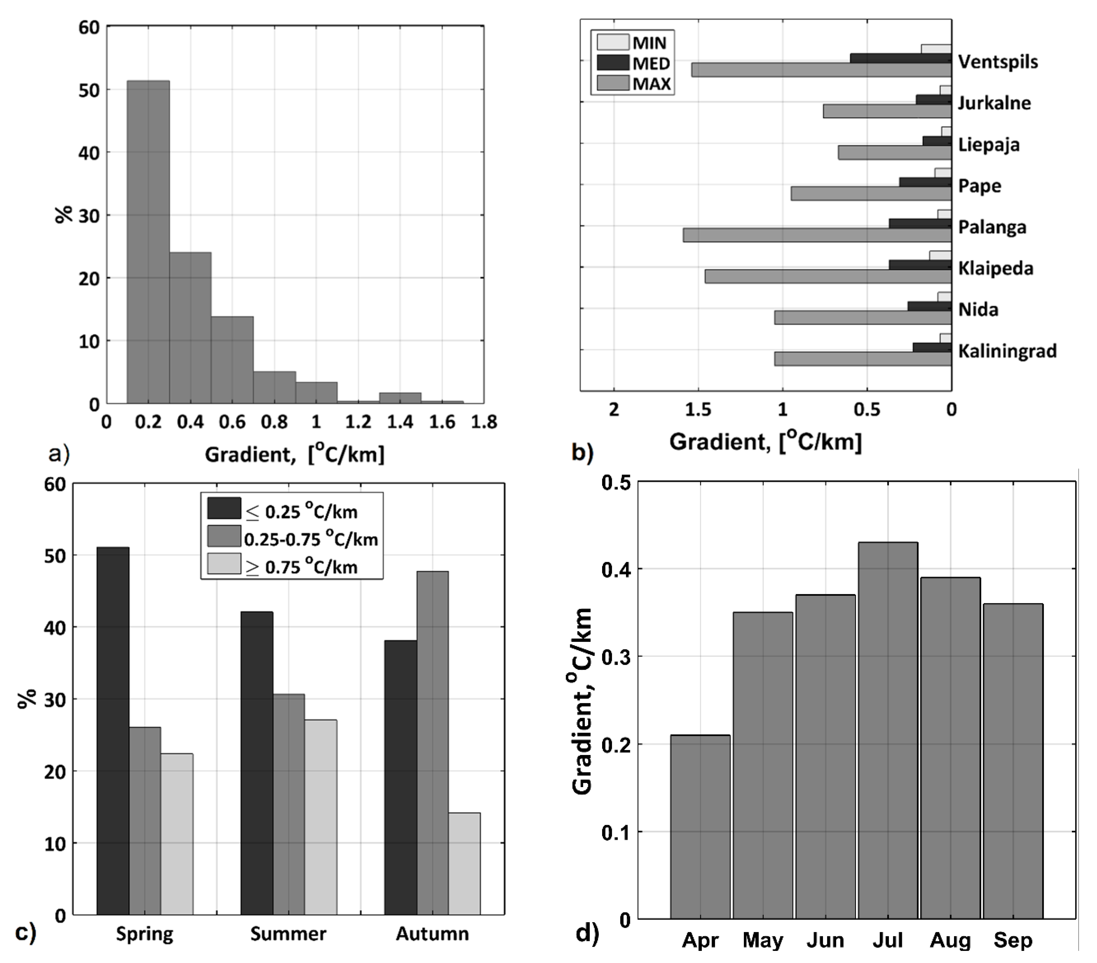
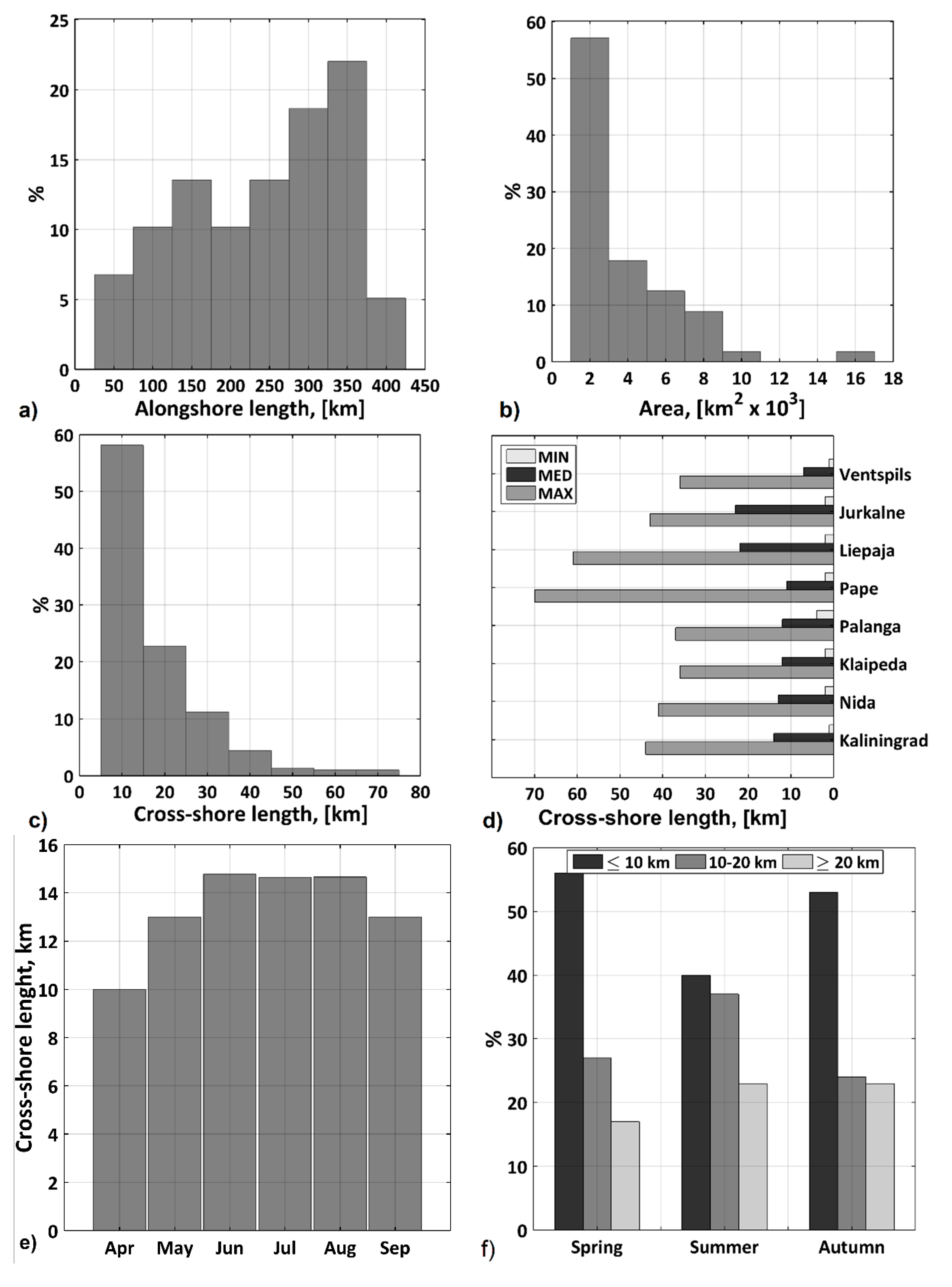
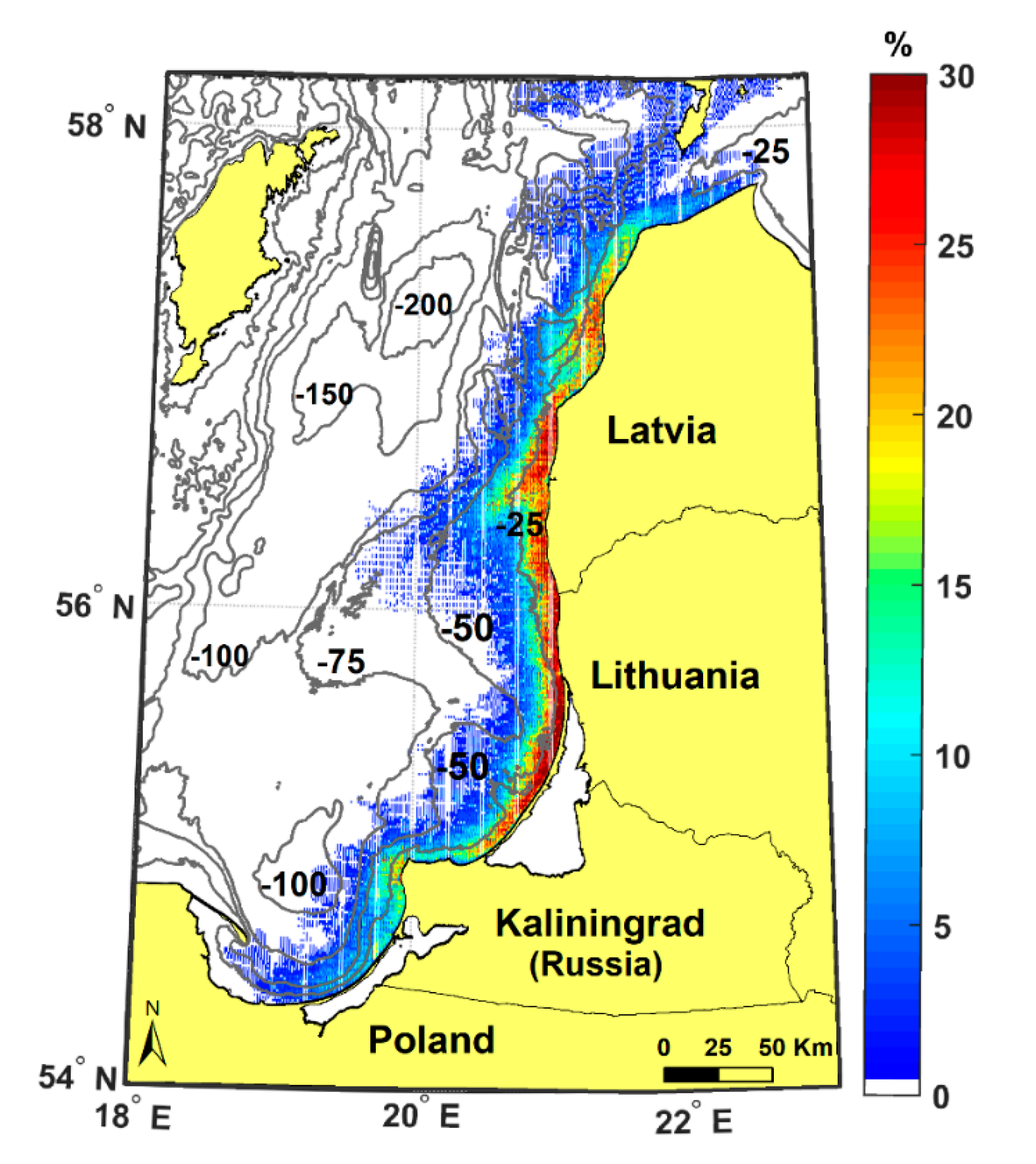
3.3.3. Spatial Properties of the Upwelling Front

As Figure 9a shows, the observed along-shore length of the upwelling front ranges from 50 to 400 km, which is presumably governed by the direction of the upwelling-favorable winds and the local configuration of the coast. The most frequent values, of about 300–350 km, covering almost the entire coastal zone of the SE Baltic Sea, are somewhat longer than what was previously reported in the literature [2,19,33]. The area of upwelling-affected waters varies among the events, ranging from several hundred up to several thousand square kilometers. In 57% of the cases, the upwelling extent is up to 3000 km², covering mainly the Lithuanian and Latvian coastal waters. Yet it may reach up to 16,000 km² (Figure 9b) in some extreme cases, extending over a significant part of Gdansk and the eastern Gotland Basins (Figure 10).

The cross-shore extent (width) of the upwelling front in the SE Baltic Sea ranges between 5 and 70 km (Figure 9c,d). The typical mean values are 10–20 km (Figure 9d), while a 5–15 km width is observed most frequently (Figure 9c), being very close to the internal Rossby radius of 2–10 km for the Baltic Sea [42]. Similar results were also reported in the literature [2,4,33]. However, during the intensive long-lasting events, the cross-shore width of the upwelling front may exceed 30–40 km everywhere, and reach 60–70 km in some locations (Figure 9d), strongly exceeding the maximum values of the internal Rossby radius observed in the summer [49]. The formation of such a wide frontal zone is very important for enhancing the exchange of biological properties between coastal and open sea waters, and is presumably linked to the evolution of the upwelling front over the topography and the generation of elongated transverse filaments extending far offshore [22], as further shown in Figure 11.

Some distinct latitudinal differences of the upwelling cross-shore extent related to the changing bathymetry of the study site are clearly seen in Figure 9d. The maximum values of the cross-shore extent were recorded along the Latvian coast near Pape (70 km) and Liepaja (61 km). They were about 37 km from the Lithuanian coast, with slightly larger values observed next to Nida (41 km). Similar values were recorded near Kaliningrad, Jurkalne, and Ventspils.

Similar to other upwelling properties, the monthly mean upwelling cross-shore extent also has some seasonal variation, rising from 10 km in April up to 15 km during summer months (Figure 9e). The portion of narrow upwelling fronts (<10 km wide) clearly dominates in the spring and autumn months, and wider upwelling fronts (>10–20 km) are observed in the summer (Figure 9f).

Figure 10 shows a map of the coastal upwelling frequency in the SE Baltic Sea derived from the space-borne SST measurements taken between 2000 and 2015. The frequency map was calculated as a ratio between the sum of the upwelling-affected pixels, recorded at every 1 × 1 km grid cell for every single upwelling event at the time of its maximal spatial development, and the total number of upwelling events.

As seen, the coastal upwelling developing under northerly winds has a typical width of the frontal zone of around 10–20 km, and covers the entire Lithuanian and Latvian coasts in 30% of the cases. It is also rather frequent near Kaliningrad, but not so pronounced along the Polish and northern Latvian coasts, having different geographic orientations (see Figure 10).

The overall pattern shown in Figure 10 is somewhat similar to the one drawn in the literature [19]. The frontal zone has numerous filamentary features located between 20° and 21°E, spreading up to 50–70 km offshore along isobaths (see Figure 11 for more details). The generation of such cold-water jets and transverse filaments was reported earlier [9,19,22], but the length reported was twice as short as the one recorded here. For any upwelling of a moderate intensity, one would observe similar characteristics—it starts just in the vicinity of the coast, and then spreads toward the open sea following the bathymetry contours. More details of the upwelling front development and evolution are presented below, considering the major coastal upwelling event that took place in the summer of 2006.

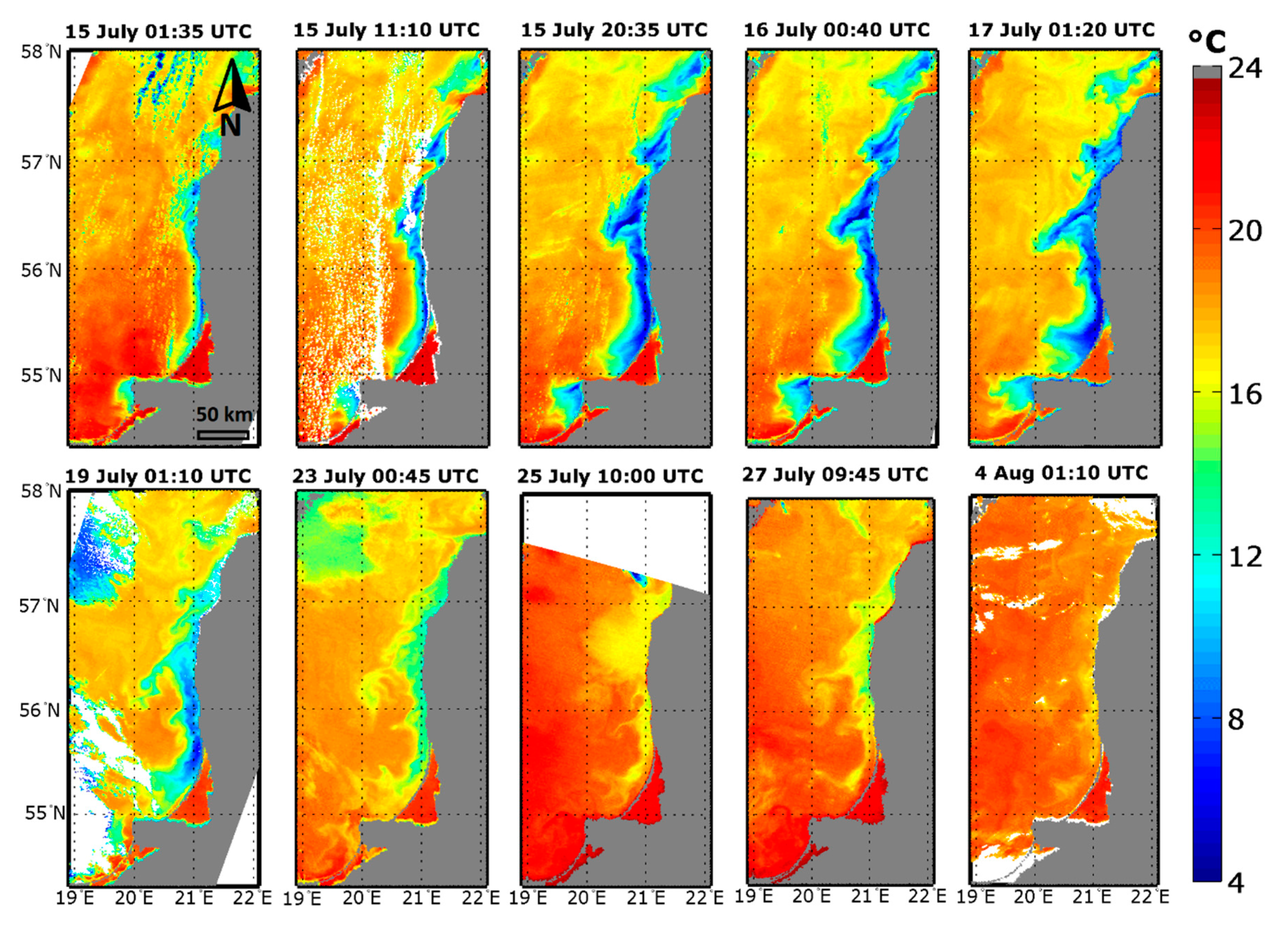
3.4. Major Upwelling Event in the Summer of 2006

An analysis of 16-year satellite observations clearly shows that a major upwelling event in the SE Baltic Sea took place in the summer of 2006 (Figure 11), similar to what was detected, for example, along the southern coast of the Gulf of Finland [18,50].

The development of this upwelling event is illustrated in Figure 11, Figure 12 and Figure 13. The available satellite data enabled the upwelling development to be captured both during the active phase, when persistent northerly winds brought cold deep waters up to the surface, and during relaxation, when the wind direction changed, but strong temperature/density gradients persisted for about two weeks.

The satellite data show the first signatures of coastal upwelling on 13 July 2006, after the northerly winds started to dominate over the study region during 10–12 July 2006 (Figure 12).

The beginning of upwelling is also well seen in water salinity (S) and air temperature (T_a) records made at Nida and Palanga coastal stations (Figure 13). An increase in salinity comes with a rapid drop of water temperature (T_w), marking the beginning of the upwelling event. An adjustment of the marine atmosphere boundary layer to the presence of the cold upwelling front is also clearly seen in T_a profiles (Figure 13) nicely following a sudden drop of water temperature at both stations.

As further seen, an intensive rise of cold deep waters up to the sea surface was observed between 15–17 July 2006. During this period, the temperature of the cold upwelling core at the surface was as low as 5–7 °С, while the associated SST difference between the ambient and upwelling waters was up to 14 °С (Figure 11). The largest increase of salinity was observed at both coastal stations during 14–21 July, and coincided with the maximal drop of T_w. However, these salinity changes were relatively small, ∆S ≤ 0.5% in agreement with the literature [39], suggesting that the surface salinity changes during the upwelling events in the Baltic Sea usually do not exceed 0.5%

Figure 13 further shows that the cooling of the surface waters is responsible for the air temperature drop down to 10 °С, and so is prone to affecting the formation and frequency of sea fog [42,51]. The latter, in turn, might have implications for the Klaipeda Port activities in terms of a reduction of visibility, hampering and restricting the navigational abilities in the port.

During 17–18 July, the wind direction changed (Figure 12), and the upwelling entered the relaxation phase, accompanied by a gradual SST increase and the further widening of the upwelling front. Elongated transverse filaments developed at the frontal boundary and spread up for about 70 km seaward. Later, these filamentary jets became unstable, meandered, and evolved into cyclonic eddies that detached from the main upwelling front on 23 July (see Figure 11). At the same time, the salinity gradually began to settle and the air temperature increased, even though, as the satellite data show in Figure 11, the cold upwelling waters persisted for about two more weeks.

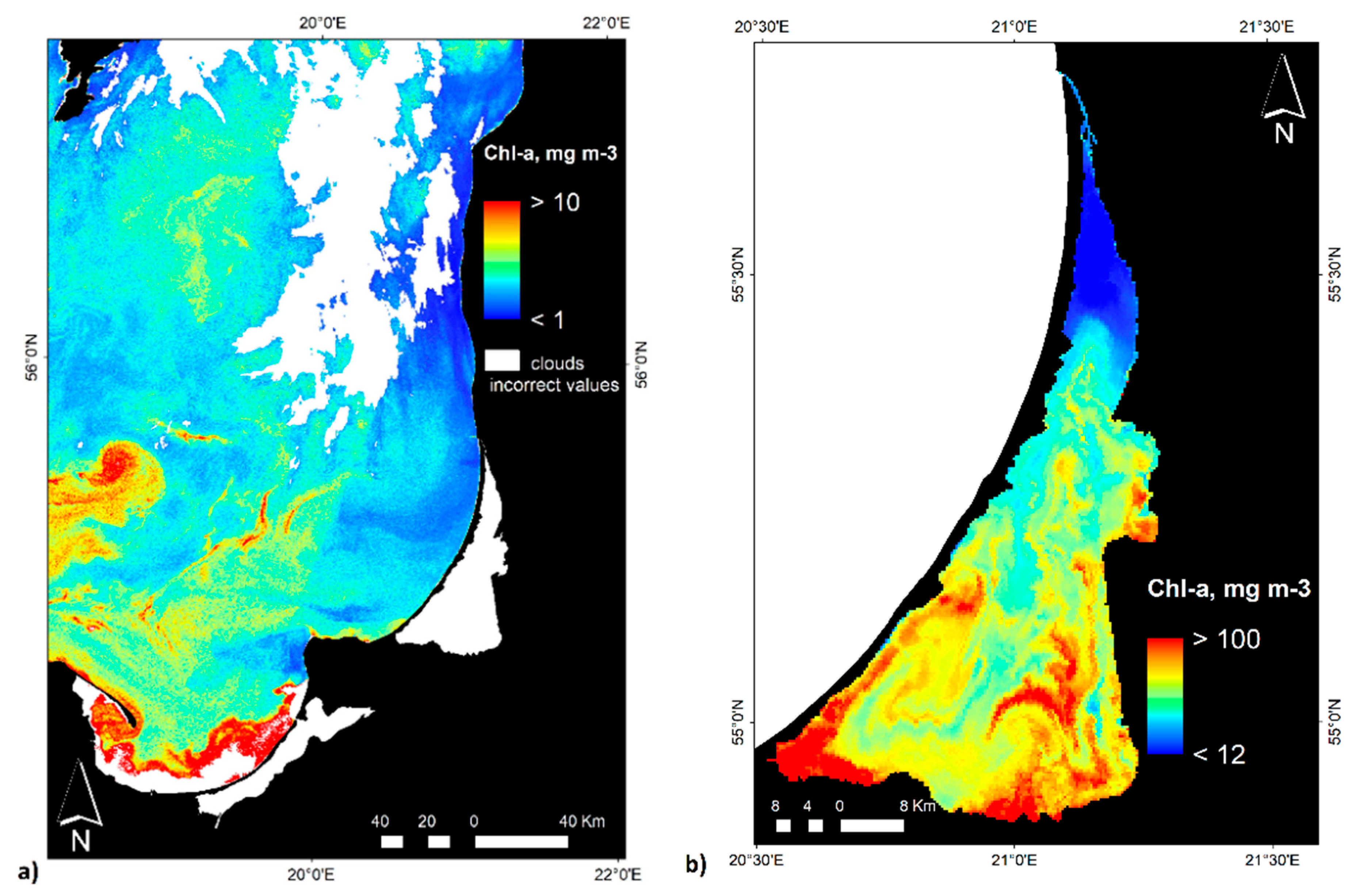
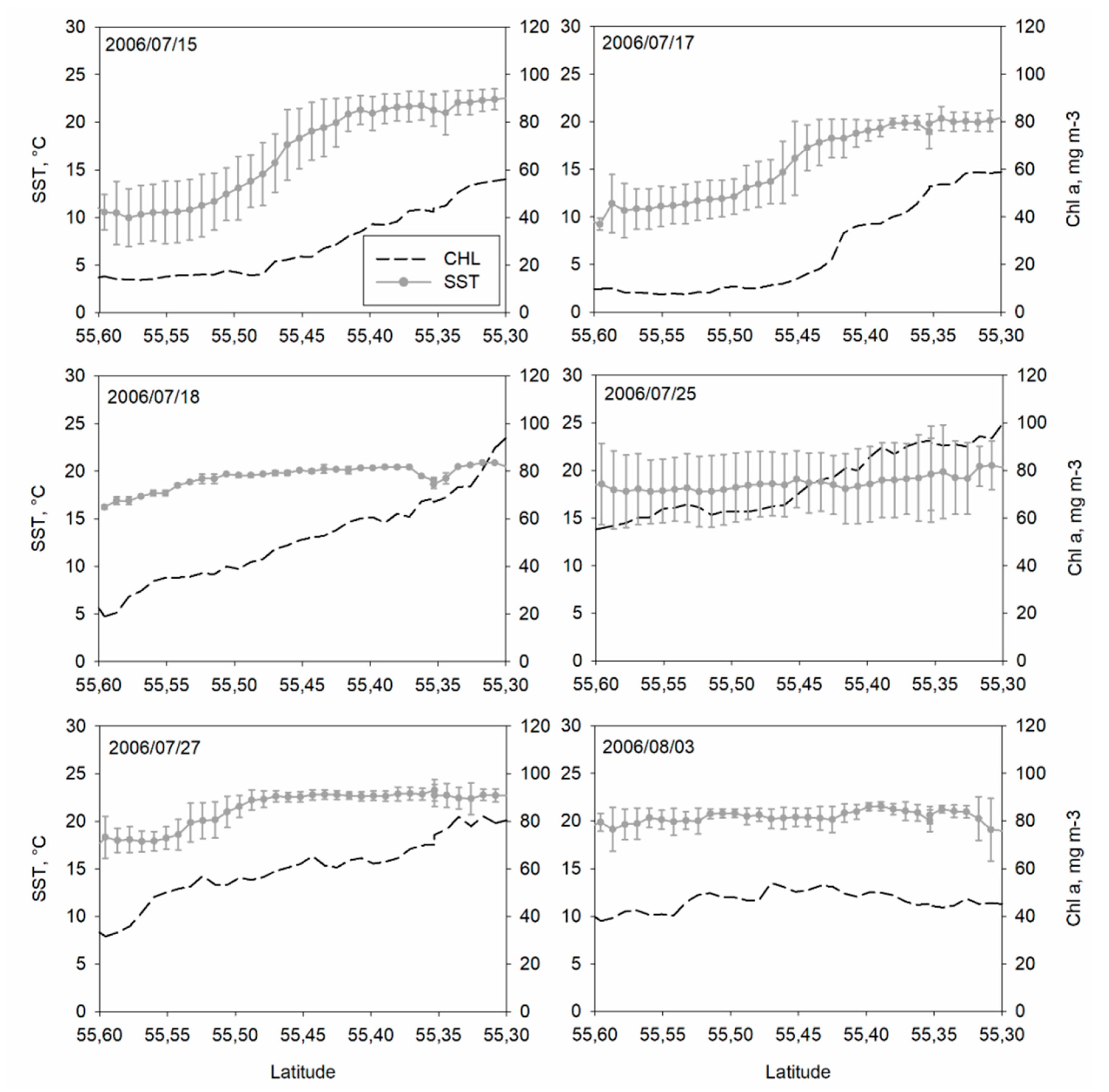
3.4.1. Upwelling Influence on the chl-a Concentration in the SE Baltic and in the Curonian Lagoon

As has already been mentioned, a wind-driven upwelling in the Baltic Sea may occur at any time of the year, although the thermal effects may not be noticeable when the sea waters are not thermally stratified [46], and upwelling may have no significant biological impact [52]. On the other hand, upwelling events during the warm season are of great importance and are recognized as efficient contributors to the exchange processes between the coastal and offshore waters [53]. At an early development stage of upwelling, more productive and turbid surface waters are often washed away from the shore, causing a significant increase in water transparency [54]. Changes in the chl-a concentration during the upwelling events were recorded along the Polish coast of the Baltic Sea [11]. The results based on a time series of synoptic SeaWiFS images revealed significantly higher chl-a concentrations during non-upwelling periods than during upwelling events in the Hel, Łeba, and Kołobrezeg regions.

In addition to the analysis of the SST data, we further determined whether the ecosystem productivity of the study area might be influenced by the coastal upwelling. Figure 14 illustrates the effect of upwelling on the spatial distribution of chl-a in the SEB coastal zone and the Curonian Lagoon during the major event in the summer of 2006. As retrieved from the satellite images acquired on 17 July 2006, a clear decline of the chl-a concentration is observed in the coastal zone (<1 mg m⁻³), relative to the ambient waters (~2.5 mg m⁻³) that are not affected by upwelling. Upwelling, at the same time (July–August 2006) taking place in the Gulf of Finland, was investigated in terms of the MERIS-derived chl-a maps [55]. A detailed spatio-temporal analysis reviled the evident influence of upwelling on the chl-a concentration, with relatively lower values during the upwelling and a significant increase during the relaxation phase, most likely because of the proliferation of phytoplankton promoted by the nutrient input, and the northward Ekman transport of surface waters caused by easterly wind forcing [55].

A strong chl-a gradient resulting from the inflow of the upwelled water masses was identified in the northern part of the Curonian Lagoon (Figure 14b). Here, the chl-a concentration dropped down by an order of magnitude relative to the ambient waters inside the lagoon (Figure 14 and Figure 15).

The investigation of cloud-free MERIS/Envisat images for the entire period of the intensive upwelling event in the summer of 2006 evidently reveals a temporal impact of the latter on the chl-a concentration in the Curonian Lagoon (Figure 15). Cold and less productive sea waters entering the lagoon pushed away and diluted the highly productive waters of the lagoon as early as on 15 July 2006. The temporal changes of the chl-a concentration derived from the MERIS/Envisat data along the transect in the lagoon (see Figure 1) also illustrates the active and relaxation phases of upwelling (Figure 15). The large upwelling-related drop of the chl-a concentration from ~60 mg m⁻³ to ~5–10 mg m⁻³ was observed on 17 July, when the upwelling was still in its active phase, and an intense rise of cold deep waters was observed along the SEB coast (Figure 11). After a few days of upwelling inflow to the lagoon, the maximum chl-a concentration in the lagoon rose from ~60 mg m⁻³ to 90–100 mg m⁻³ (Figure 15). Unlike the SST profile that almost returned to its pre-upwelling values during 18–25 July, chl-a had a very distinct sloping profile until it stabilized around a nearly constant value of 45 mg m⁻³ on 3 August 2016. As a result, the overall drop in the background chl-a concentration before and after the upwelling event was ~15 mg m⁻³.

On the other hand, nutrient-rich water masses brought from the deeper layers to the surface, and the higher level of available radiation, significantly enhanced the primary production [10,11,56] and caused changes in the phytoplankton community during the coastal upwelling events [12,57,58]. These changes and the rate of production, however, depend on various environmental variables (e.g., season, water temperature, concentration of nutrients, weather conditions), and are of great importance to the entire coastal environment, and therefore should be addressed in future studies.

3.4.2. Upwelling Impact on Near-Surface Wind Field

As mentioned in Section 3.4.1, the presence of a cold upwelling front along the SEB coast has a direct impact on the near-surface air temperature (Figure 13) associated with the marine atmosphere boundary layer (MABL) adjustment to the local SST across the upwelling front. The cold upwelling front alters the stratification in the MABL, which becomes more stable, and subsequently lowers the near-surface wind speed and surface stress [9,59,60]. The suppression of near-surface wind speed over the cold sector of the front is well demonstrated in Figure 16, where SST maps are shown together with time-collocated high-resolution SAR-derived wind field maps.

The wind field map acquired on 16 July 2006 shows background northerly winds of 4–7 m s⁻¹ over the study site (Figure 16b). As can be seen, the wind speed over the cold water in the upwelling region drops to 2–4 m s⁻¹ as the MABL stratification becomes stable. The SAR-based wind map of 19 July 2006 exhibits the presence of an atmospheric front that intercepts the upwelling area (Figure 16d). This wind front is partly accompanied by a 50-km-wide band of clouds (Figure 16c) that mask the thermal expressions in the SST map in a northwesterly direction. Note that, unlike the SST data affected by clouds, the SAR-derived wind maps provide valuable information on the thermal front location over the cloud-contaminated region, and clearly demonstrate the upwelling-induced wind speed changes in the MABL (Figure 16d). In the upper part of the SAR-wind image, the northeasterly winds range from 4 to 6 m s⁻¹, whereas the lower part of the map is characterized by light winds. Here, again, one can see a clear drop in the wind speed down to calm conditions in the lower part of the wind map, and down to 1–3 m s⁻¹ in the upper part (Figure 16d).

The impact of the Baltic Sea upwelling on the atmosphere boundary layer in a wider context was detailed in a model study in the literature [31]. In particular, the authors show that the upwelling influence is generally small, and results in only small changes in the summer-mean conditions of the boundary layer (i.e., 2-m height air temperature reductions of up to 2 °C, wind speed reductions of up to 0.25 m s⁻¹, and reductions in mean boundary layer height of up to 100 m). Nevertheless, they importantly point out that the upwelling influence can be significant locally over areas where upwelling is the most common. Given that the upwelling frequency is rather high along the SEB during the warm half of the year, the reported upwelling-induced reduction of wind speed by 2–4 m s⁻¹ in the coastal zone seems to be important (e.g., for offshore and near-shore wind farming that is planned in this area in the near future).

4. Summary and Conclusions

This study provides a detailed analysis of wind-induced coastal upwelling and its properties in the SE Baltic Sea based on multi-mission satellite data. Upwelling events were detected during the thermally stratified season between April and September, with the earliest registered on 14 April 2010 and the latest on 23 September 2008. About 90% of events were observed between May and August, with a clear peak in July characterized by eight upwelling days on average. For the high upwelling season from May to August, the monthly average value is about seven upwelling days per month, or 20–25% of the month.

An evaluation of the Ekman-based upwelling index enabled the identification of 96 upwelling events, meaning that the satellite-based CU detection represents about 72% of the total of all possible upwelling events. The use of satellite data is more effective during May–August, allowing for the observation of about 87% of all UI-based upwelling events under relatively cloud-free summer conditions. In general, about one to three days of positive UI values are needed for the upwelling front to be manifested in the SST data. As has been found, the milder upwelling-favorable winds of a shorter duration are required to cause upwelling during the summer months when the seasonal thermocline is shallow and the vertical stratification of the water column is at its strongest, and a longer and stronger wind impulse is needed in the spring and early autumn.

The obtained results show that short-lived upwelling events that are two to six days long clearly dominate in the record, while about 27% of the events persist for seven to ten days. In some distinct cases, the coastal upwelling may last up to 23 days, as a result of a chain of consecutive upwelling events. The frequency of coastal upwelling ranged from one to several events per year, occurring about four times per season on average. The longest upwelling season was up to 57 days per year, covering about 30% of the warm period.

As has been further shown, no significant latitudinal differences in upwelling-induced ∆T values along the SEB coast were observed with maximum and median values of about 12 °C and 4 °C, respectively. At the same time, considerable spatial variations of the SST gradient were observed with a maximum value of about 1.5 °C km⁻¹. In the summer and autumn months, higher SST gradients clearly prevail, while the highest values (more than 0.75 °C km⁻¹) are observed more frequently in the summer than in the spring or autumn.

The most frequent values of the along-shore length of the upwelling front are about 300–350 km, covering almost the entire coastal zone of the SE Baltic Sea. In 57% of the cases, the upwelling extent is up to 3000 km², covering mainly the Lithuanian and Latvian coastal waters. Yet, it may reach up to 16,000 km² during some extreme events, extending over a significant part of Gdansk and the eastern Gotland Basins.

The cross-shore extent of the upwelling front in the SE Baltic Sea ranges between 5 and 70 km, yet during intensive long-lasting events, it may exceed 30–40 km everywhere, and reach 60–70 km in some locations. This is quite significant considering that the average width of the Baltic Sea is around 190 km. Furthermore, the generation of such filamentary patterns results in mixing between coastal and open waters, and enhances the exchange of biological properties between them. The maximum values of the cross-shore extent are recorded along the Latvian coast near Pape (70 km) and Liepaja (61 km). The generation of such cold-water jets and transverse filaments was reported earlier, but the length that was reported was twice as short as the one recorded here.

An analysis of the satellite optical data during the major upwelling event in the summer of 2006 clearly shows a clear three-fold decrease in the chl-a concentration in the coastal zone, relative to the ambient waters. Similarly, a strong chl-a gradient resulting from the inflow of upwelled water masses is identified in the northern part of the Curonian Lagoon, where the chl-a concentration drops down by an order of magnitude. As a result, the overall drop in the background chl-a concentration in the Curonian Lagoon before and after an upwelling event is ~15 mg m⁻³.

As has been further shown, the presence of a cold upwelling front might significantly alter the stratification of the marine atmosphere boundary layer and result in a significant drop of air temperature and near-surface winds in the coastal zone. As such, it is prone to affect the formation and frequency of sea fog, which might have implications for the Klaipeda Port activities as well as the offshore and near-shore wind farming that is planned in this area in the near future.

The study outcomes suggest that the satellite-derived SST, wind, and chl-a products could be used to analyze the intensity of the coastal upwelling and its biological and atmospheric response, and, moreover, yield significant information about sea–lagoon interaction.

References

1. Plattner, S.; Mason, D.M.; Leshkevich, G.A.; Schwab, D.J.; Rutherford, E.S. Classifying and Forecasting Coastal Upwellings in Lake Michigan Using Satellite Derived Temperature Images and Buoy Data. J. Great Lakes Res. 2006, 32, 63–76. [Google Scholar] [CrossRef] [Green Version]
2. Lehmann, A.; Myrberg, K.; Hoflich, K. A statistical approach to coastal upwelling in the Baltic Sea based on the analysis of satellite data for 1990–2009. Oceanologia 2012, 54, 369–393. [Google Scholar] [CrossRef] [Green Version]
3. Sproson, D.; Sahlée, E. Modelling the impact of Baltic Sea upwelling on the atmospheric boundary layer. Tellus A Dyn. Meteorol. Oceanogr. 2014, 66. [Google Scholar] [CrossRef] [Green Version]
4. Lehmann, A.; Myrberg, K. Upwelling in the Baltic Sea—A review. J. Mar. Syst. 2008, 74, S3–S12. [Google Scholar] [CrossRef] [Green Version]
5. Zhurbas, V.; Laanemets, J.; Vahtera, E. Modeling of the mesoscale structure of coupled upwelling/downwelling events and the related input of nutrients to the upper mixed layer in the Gulf of Finland, Baltic Sea. J. Geophys. Res. 2008, 113. [Google Scholar] [CrossRef] [Green Version]
6. Kahru, M.; Hakansson, B.; Rud, O. Distributions of the sea-surface temperature fronts in the Baltic Sea as derived from satellite imagery. Cont. Shelf Res. 1995, 15, 663–679. [Google Scholar] [CrossRef]
7. Alenius, P.; Myrberg, K.; Nekrasov, A. The physical oceanography of the Gulf of Finland: A review. Boreal Environ. Res. 1998, 3, 97–125. [Google Scholar]
8. Fuchs, R.; Pinazo, C.; Douillet, P.; Fraysse, M.; Grenz, C.; Mangin, A.; Dupouy, C. Modelling ocean–lagoon interaction during upwelling processes in the South West of New Caledonia. Estuar. Coast. Shelf Sci. 2013, 135, 5–17. [Google Scholar] [CrossRef]
9. Kozlov, I.E.; Kudryavtsev, V.N.; Johannessen, J.A.; Chapron, B.; Dailidiene, I.; Myasoedov, A.G. ASAR imaging for coastal upwelling in the Baltic Sea. Adv. Space Res. 2012, 50, 1125–1137. [Google Scholar] [CrossRef]
10. Kowalewski, M. The influence of the Hel upwelling (Baltic Sea) on nutrient concentrations and primary production—The results of an ecohydrodynamic model. Oceanologia 2005, 47, 567–590. [Google Scholar]
11. Krężel, A.; Szymanek, L.; Kozłowski, Ł.; Szymelfenig, M. Influence of coastal upwelling on chlorophyll a concentration in the surface water along the Polish coast of the Baltic Sea. Oceanologia 2005, 47, 433–452. [Google Scholar]
12. Vahtera, E.; Laanemets, J.; Pavelson, J.; Huttunen, M.; Kononen, K. Effect of upwelling on the pelagic environment and bloom-forming cyanobacteria in the western Gulf of Finland, Baltic Sea. J. Mar. Syst. 2005, 58, 67–82. [Google Scholar] [CrossRef]
13. Schernewski, G.; Behrendt, H.; Neumann, T. An integrated river basin-coast-sea modelling scenario for nitrogen management in coastal waters. J. Coast. Conserv. 2008, 12, 53–66. [Google Scholar] [CrossRef]
14. Baltic Earth. Available online: https://www.baltic-earth.eu/ (accessed on 1 September 2018).
15. Jiang, L.; Breaker, L.C.; Yan, X.-H. A model for estimating cross-shore surface transport with application to the New Jersey Shelf. J. Geophys. Res. 2010, 115. [Google Scholar] [CrossRef] [Green Version]
16. Klemas, V. Remote Sensing Techniques for Studying Coastal Ecosystems: An Overview. J. Coast. Res. 2011, 27, 2–17. [Google Scholar] [CrossRef] [Green Version]
17. Gurova, E.; Lehmann, A.; Ivanov, A. Upwelling dynamics in the Baltic Sea studied by a combined SAR/infrared satellite data and circulation model analysis. Oceanologia 2013, 55, 687–707. [Google Scholar] [CrossRef] [Green Version]
18. Uiboupin, R.; Laanemets, J. Upwelling characteristics derived from satellite sea surface temperature data in the Gulf of Finland, Baltic Sea. Boreal Environ. Res. 2009, 14, 297–304. [Google Scholar]
19. Bychkova, I.; Viktorov, S. Use of satellite data for identification and classification of upwelling in the Baltic Sea. Oceanology 1987, 27, 158–162. [Google Scholar]
20. Myrberg, K.; Andrejev, O. Main upwelling regions in the Baltic Sea—A statistical analysis based on three-dimensional modelling. Boreal Environ. Res. 2003, 8, 97–112. [Google Scholar]
21. Bychkova, I.; Viktorov, S.; Shumakher, D.A. A relationship between the large-scale atmospheric circulation and the origin of coastal upwelling in the Baltic Sea. Meteorol. Gidrol. 1988, 10, 91–98. [Google Scholar]
22. Zhurbas, V.M.; Stipa, T.; Mälkki, P.; Paka, V.T.; Kuzmina, N.P.; Sklyarov, E.V. Mesoscale variability of the upwelling in the southeastern Baltic Sea: IR images and numerical modelling. Oceanology 2004, 44, 619–628. [Google Scholar]
23. Zhurbas, V.; Oh, I.S.; Park, T. Formation and decay of a longshore baroclinic jet associated with transient coastal upwelling and downwelling: A numerical study with applications to the Baltic Sea. J. Geophys. Res. 2006, 111. [Google Scholar] [CrossRef] [Green Version]
24. Golenko, M.N.; Golenko, N.N. Structure of dynamic fields in the Southeastern Baltic during wind forcings that cause upwelling and downwelling. Oceanology 2012, 52, 604–616. [Google Scholar] [CrossRef]
25. Brown, O.B.; Minnett, P.J. MODIS Infrared Sea Surface Temperature Algorithm; Tech. Report ATBD25, FL 33149-1098; University of Miami: Coral Gables, FL, USA, 1999. [Google Scholar]
26. NASA OceanColor Website. Available online: https://oceancolor.gsfc.nasa.gov/ (accessed on 1 September 2018).
27. Kozlov, I.; Dailidiene, I.; Korosov, A.; Klemas, V.; Mingelaite, T. MODIS-based sea surface temperature of the Baltic Sea Curonian Lagoon. J. Mar. Syst. 2014, 129, 157–165. [Google Scholar] [CrossRef]
28. Vaičiūtė, D.; Bresciani, M.; Bučas, M. Validation of Meis bio-optical products with in situ data in the turbid Lithuanian Baltic Sea coastal waters. J. Appl. Remote Sens. 2012, 6, 1–20. [Google Scholar] [CrossRef]
29. Giardino, C.; Bresciani, M.; Pilkaitytė, R.; Bartoli, M.; Razinkovas, A. In situ measurements and satellite remote sensing of case 2 waters: First results from the Curonian Lagoon. Oceanologia 2010, 52, 197–210. [Google Scholar] [CrossRef]
30. Bresciani, M.; Giardino, C.; Stroppiana, D.; Pilkaitytė, R.; Zilius, M.; Bartoli, M.; Razinkovas, A. Retrospective analysis of spatial and temporal variability of chlorophyll-a in the Curonian Lagoon. J. Coast. Conserv. 2012, 16, 511–519. [Google Scholar] [CrossRef]
31. INFORM. INFORM Prototype/Algorithm Validation Report Update. 2016. D5.15. p. 140. Available online: http://inform.vgt.vito.be/files/documents/INFORM_D5.15_v1.0.pdf (accessed on 5 November 2018).
32. Stoffelen, A.; Anderson, D. Scatterometer data interpretation: Estimation and validation of the transfer function CMOD4. J. Geophys. Res. 1997, 102, 5767–5780. [Google Scholar] [CrossRef] [Green Version]
33. Gidhagen, L. Coastal upwelling in the Baltic Sea—Satellite and in situ measurements of sea-surface temperatures indicating coastal upwelling. Estuar. Coast. Shelf Sci. 1987, 24, 449–462. [Google Scholar] [CrossRef]
34. Bakun, A. Coastal Upwelling Indices, West Coast of North America, 1946–71; NOM Tech. Rep. NMFS SSRF-671; Scientific Publications Office: Seattle, WA, USA, 1973; 103p. [Google Scholar]
35. Chenillat, F.; Riviere, P.; Capet, X.; Di Lorenzo, E.; Blanke, E. North Pacific Gyre Oscillation modulates seasonal timing and ecosystem functioning in the California Current upwelling system. Geophys. Res. Lett. 2012, 39. [Google Scholar] [CrossRef]
36. Bograd, S.J.; Schroeder, I.; Sarkar, N.; Qiu, X.; Sydeman, W.J.; Schwing, F.B. Phenology of coastal upwelling in the California Current. Geophys. Res. Lett. 2009, 36. [Google Scholar] [CrossRef] [Green Version]
37. Gomez-Gesteira, M.; Moreira, C.; Alvarez, I.; deCastro, M. Ekman transport along the Galician coast (northwest Spain) calculated from forecasted winds. J. Geophys. Res. 2006, 111. [Google Scholar] [CrossRef] [Green Version]
38. Cropper, T.E.; Hanna, E.; Bigg, G.R. Spatial and temporal seasonal trends in coastal upwelling off Northwest Africa, 1981–2012. Deep-Sea Res. I 2014, 86, 94–111. [Google Scholar] [CrossRef]
39. Haapala, J. Upwelling and its Influence on Nutrient Concentration in the Coastal Area of the Hanko Peninsula, Entrance of the Gulf of Finland. Estuar. Coast. Shelf Sci. 1994, 38, 507–521. [Google Scholar] [CrossRef]
40. Myrberg, K.; Lehmann, A. Topography, Hydrography, Circulation and Modelling of the Baltic Sea. In Preventive Methods for Coastal Protection: Towards the Use of Ocean Dynamics for Pollution Control; Soomere, T., Quak, E., Eds.; Springer: Berlin, Germany, 2013; pp. 31–64. [Google Scholar]
41. Jurkin, V.; Kelpsaite, L. Upwelling by the Lithuanian coast: Numerical prediction using GIS methods. IEEE/OES Balt. Int. Symp. 2012. [Google Scholar] [CrossRef]
42. Leppäranta, M.; Myrberg, K. Physical Oceanography of the Baltic Sea; Springer-Praxis: Heidelberg, Germany, 2009; ISBN 978-3-540-79702-9. [Google Scholar]
43. Soomere, T.; Keevallik, S. Directional and extreme wind properties in the Gulf of Finland. Proc. Est. Acad. Sci. Eng. 2003, 9, 73–90. [Google Scholar]
44. Karstensen, J.; Liblik, T.; Fisher, J.; Bumke, K.; Krahmann, G. Summer upwelling at the Boknis Eck time-series station (1982 to 2012)—A combined glider and wind data analysis. Biogeosciences 2014, 11, 3603–3617. [Google Scholar] [CrossRef] [Green Version]
45. Myrberg, K.; Andrejev, O.; Lehmann, A. Dynamic features of successive upwelling events in the Baltic Sea—A numerical case study. Oceanologia 2010, 52, 77–99. [Google Scholar] [CrossRef]
46. Bednorz, E.; Półrolniczak, M.; Czernecki, B. Synoptic conditions governing upwelling along the Polish Baltic coast. Oceanologia 2013, 55, 767–785. [Google Scholar] [CrossRef]
47. Iles, A.C.; Gouhier, T.C.; Menge, B.A.; Stewart, J.S.; Haupt, A.J.; Lynch, M.C. Climate-driven trends and ecological implications of event-scale upwelling in the California Current System. Glob. Chang. Biol. 2012, 18, 783–796. [Google Scholar] [CrossRef]
48. Esiukova, E.E.; Chubarenko, I.P.; Stont, Z.I. Upwelling or Differential Cooling? Analysis of Satellite SST Images of the Southeastern Baltic Sea. Water Resour. 2017, 44, 69–77. [Google Scholar] [CrossRef]
49. Fennel, W.; Seifert, T.; Kayser, B. Rossby radii and phase speeds in the Baltic Sea. Cont. Shelf Res. 1991, 11, 23–36. [Google Scholar] [CrossRef]
50. Suursaar, U.; Aps, R. Spatio-temporal variations in hydro-physical and -chemical parameters during a major upwelling event off the southern coast of the Gulf of Finland in summer 2006. Oceanologia 2007, 49, 209–228. [Google Scholar]
51. Dietze, H.; Loptien, U. Effects of surface current–wind interaction in an eddy-rich general ocean circulation simulation of the Baltic Sea. Ocean Sci. 2016, 12, 977–986. [Google Scholar] [CrossRef] [Green Version]
52. Pisoni, J.P.; Rivas, A.L.; Piola, A.R. Satellite remote sensing reveals coastal upwelling events in the San Matías Gulf—Northern Patagonia. Remote Sens. Environ. 2014, 152, 270–278. [Google Scholar] [CrossRef]
53. Lévy, M. The Modulation of Biological Production by Oceanic Mesoscale Turbulence. In Transport and Mixing in Geophysical Flows; Lecture Notes in Physics; Weiss, J.B., Provenzale, A., Eds.; Springer: Berlin/Heidelberg, Germany, 2008; Volume 744, pp. 219–261. [Google Scholar]
54. Nowacki, J.; Matciak, M.; Szymelfenig, M.; Kowalewski, M. Upwelling characteristics in the Puck Bay (the Baltic Sea). Oceanol. Hydrobiol. Stud. 2009, 38, 3–16. [Google Scholar] [CrossRef]
55. Uiboupin, R.; Laanemets, J.; Sipelgas, L.; Raag, L.; Lips, I.; Buhhalko, N. Monitoring the effect of upwelling on the chlorophyll a distribution in the Gulf of Finland (Baltic Sea) using remote sensing and in situ data. Oceanologia 2012, 54, 395–419. [Google Scholar] [CrossRef]
56. Cravo, A.; Relvas, P.; Cardeira, S.; Rita, F.; Madureira, M.; Sanches, R. An upwelling filament off southwest Iberia: Effect on the chlorophyll a and nutrient export. Cont. Shelf Res. 2010, 30, 1601–1613. [Google Scholar] [CrossRef]
57. Gromisz, S.; Szymelfenig, M. Phytoplankton in the Hel upwelling Region (the Baltic Sea). Oceanol. Hydrobiol. Stud. 2005, 34, 115–135. [Google Scholar]
58. Kanoshina, I.; Lips, U.; Leppänen, J.-M. The influence of weather conditions (temperature and wind) on cyanobacterial bloom development in the Gulf of Finland (Baltic Sea). Harmful Algae 2003, 2, 29–41. [Google Scholar] [CrossRef]
59. Kudryavtsev, V.N.; Grodsky, S.A.; Dulov, V.A.; Malinovsky, V.V. Observations of atmospheric boundary layer evolution above the Gulf Stream frontal zone. Bound.-Layer Meteorol. 1996, 79, 51–82. [Google Scholar] [CrossRef]
60. Kudryavtsev, V.; Kozlov, I.; Chapron, B.; Johannessen, J.A. Quad-polarization SAR features of ocean currents. J. Geophys. Res. 2014, 119, 6046–6065. [Google Scholar] [CrossRef] [Green Version]
Figure 1. Map of the study site in the south-eastern (SE) Baltic Sea showing the locations of the cross-frontal transects and hydrometeorological stations (HMS).
Remotesensing 10 01752 g001
Figure 2. Overall number of upwelling events identified in the satellite infrared (IR) imagery (denoted as SST, for sea surface temperature), from the water temperature (Tw) measurements at the Klaipeda monitoring station and based on the upwelling index (UI) in the SE Baltic Sea from April to September 2000–2015. The blue line with diamonds shows the number of satellite images available per month.
Remotesensing 10 01752 g002
Figure 3. Typical SST and bathymetry profiles in the Baltic Sea near Pape, Klaipeda, and Nida. The green-dashed line denotes the spring SST, the red solid line denotes the summer SST, and the blue dotted line denotes the autumn SST. The black solid line corresponds to the bathymetry profiles (denoted as “Depth”).
Remotesensing 10 01752 g003
Figure 4. Monthly wind roses for April–September 2000–2015, based on the data from the Klaipeda coastal meteorological station. Wind directions framed in red indicate upwelling favorable winds.
Remotesensing 10 01752 g004
Figure 5. Meteorological conditions prior to coastal upwelling development in the SE Baltic Sea. (a) Number of days with positive UI values before the first manifestation of coastal upwelling in thee satellite data; (b) cumulative upwelling index for all of the coastal upwelling events identified in the satellite data; (c) seasonal distribution of (a,b).
Remotesensing 10 01752 g005aRemotesensing 10 01752 g005b
Figure 6. Upwelling season and duration in the SE Baltic Sea in 2000–2015: (a) Total number of upwelling events/days with upwelling per single month; (b) Histogram of upwelling duration; (c) Interannual changes of upwelling duration and frequency.
Remotesensing 10 01752 g006
Figure 7. Upwelling induced SST modulations for the period 2000–2015: (a) upwelling induced SST drop (∆T); (b) spatial distribution of ∆T along the SE Baltic (SEB) coast; (c) mean monthly ∆T; (d) seasonal changes of ∆T.
Remotesensing 10 01752 g007
Figure 8. Upwelling-induced SST gradients for the period 2000–2015: (a) histogram of horizontal SST gradients; (b) spatial distribution of SST gradients along the SEB coast; (c) seasonal changes of SST gradients; (d) mean monthly SST gradients.
Remotesensing 10 01752 g008
Figure 9. Spatial properties of coastal upwelling front in the SE Baltic Sea. Histogram distributions of (a) along-shore length; (b) upwelling area; (c) cross-shore length; (d) spatial distribution of cross-shore length; (e) monthly-mean cross-shore length; and (f) seasonal variation of cross-shore length.
Remotesensing 10 01752 g009
Figure 10. The spatial frequency of coastal upwelling generated by northerly winds along the SE Baltic Sea coast. Grey lines show bathymetry contours.
Remotesensing 10 01752 g010
Figure 11. Development of a major coastal upwelling event in the SE Baltic Sea in the summer of 2006.
Remotesensing 10 01752 g011
Figure 12. Wind speed and direction recorded in July 2006 at the Palanga, Klaipeda, and Nida coastal stations. F in the left corner of each of the panels indicates upwelling-favorable northerly winds.
Remotesensing 10 01752 g012
Figure 13. Sea water temperature (Tw), air temperature (Ta), and salinity (S) changes recorded at the Nida and Palanga coastal stations in July 2006.
Remotesensing 10 01752 g013aRemotesensing 10 01752 g013b
Figure 14. Spatial distribution of the chl-a concentration during the major upwelling event, as retrieved from MERIS/Envisat (Medium Resolution Imaging Spectrometer onboard the Envisat satellite, European Space Agency) (a) in the Baltic Sea coastal waters (b) and in the Curonian Lagoon on 17 July 2006.
Remotesensing 10 01752 g014
Figure 15. Spatial distribution of SST and the chl-a concentration along the transect in the Curonian Lagoon (shown on Figure 1) during the major upwelling event in the summer of 2006. The grey line with circles indicates the mean SST derived from the Moderate Resolution Imaging Spectroradiometer (MODIS)/Aqua and MODIS/Terra images of the day, and the error bars indicate the standard deviation of the SST. The black dashed line shows the chl-a concentration derived from the MERIS data.
Remotesensing 10 01752 g015
Figure 16. Upwelling impact on the near-surface wind field in the SE Baltic Sea. (a) MODIS/Aqua SST map of 16 July 2006 (19:40 UTC); (b) synthetic aperture radar (SAR)-derived near-surface wind field of 16 July 2006 (20:05 UTC); (c) same as (a), but for 19 July 2006 (20:10 UTC); (d) same as (b), but for 19 July 2006 (20:11 UTC).
Remotesensing 10 01752 g016