Multi-Layered Local Dynamic Map for a Connected and Automated In-Vehicle System

Abstract

Automated Driving (AD) has been receiving considerable attention from industry, the public, and researchers for its ability to reduce accidents, emissions, and congestion. The purpose of this study is to extend the standardized Local Dynamic Map (LDM) by adding two new layers, and develop efficient and accurate algorithms designed to enhance AD by exploiting the LDM coupled with Cooperative Perception (CP). The LDM is implemented as a Neo4j graph database and extends the standard four-layer structure by adding a detection layer and a prediction layer. A custom Application Programming Interface (API) manages all incoming data, generates the LDM, and runs the algorithms. Currently, the API can match detected entities coming from different sources, correctly position them on the map even in the presence of high uncertainties in the data, and predict their future actions. We tested the developed LDM with real-world data, which we collected using a prototype vehicle from Centro Ricerche FIAT (CRF) Trento Branch—the supporting research center for this work—in urban, suburban, and highway areas of Trento, Italy. The results show that the developed solution is capable of accurately matching and predicting detected entities, is robust to high uncertainties in the data, and is efficient, achieving real-time performance in all scenarios. From these results we can conclude that the LDM and CP have the potential to be core parts of AD, bringing improvements to the development process.

1. Introduction

Road transport ensures the mobility of people and goods, although it still poses several challenges. For instance, the European Union’s policies address, amongst other problems, those of traffic congestion, safety, pollution and carbon footprint. The goal is to foster sustainability of road transport which is de facto the most common means of displacement in the EU [1]. One of the main research fields that is focused on these issues is Automated Driving (AD), the goal of which is to deploy Automated Vehicles (AVs) to decrease accidents, emissions, and congestion, amongst other things. Examples of AVs exist [2], but they are still far from a globally adoptable solution mainly due to their limitations in complex environments (e.g., crowded urban areas, emergency manoeuvres). Coping with the real world is one of the biggest challenges for an AV, and current research suggests that the solution could be the Cooperative Intelligent Transport Systems (C-ITSs). These systems are based on communication between vehicles, other road users, road infrastructure as well as back-end Information and Communication Technologies (ICT) systems and services, which cooperate with one another, exchanging information (e.g., positions, detections, warnings, recommendations). The enabling technology is vehicle-to-everything communication (V2X) which can be performed by the vehicle either directly with local elements such as other vehicles (V2V), road side units (V2I), vulnerable users’ devices (V2P), or indirectly through internet-based services dispatching messages to/from users (V2N). With such pre-conditions, V2X enhances and extends the AV local sensing with information such as other vehicles’ and vulnerable road users’ motion; static, temporary, and dynamic signs; traffic light phases and related timing; local high definition (HD) map elements and map changes; predicted hazards. Amongst the recently standardized messages to share V2X data, the Collective Perception Message (CPM) is an outstanding means for AV to share not only their position but also their sensed objects. Within AVs, one way to ingest and manage all this data, and in particular Collective Perception (CP) data, is through the use of the Local Dynamic Map (LDM), which is essentially a database storing information about the environment of interest.

The concept of the LDM was born from the cooperation between the SAFESPOT [3] and CVIS projects [4]. In particular, the LDM was a product of the SINTECH project, a SAFESPOT subproject, and was developed to store static/dynamic sensor and communication information after an appropriate data fusion process. The LDM was structured as a geo-referenced local database in which each node contained the aforementioned data to be served to all the applications that needed it. After these projects ended, the LDM was first introduced in the Technical Report ETSI TR 102 863 [5] in 2011 and then standardized in the European Standard ETSI EN 302 895 [6] in 2014 by the European Telecommunications Standards Institute (ETSI). The technical report defines the LDM as a

“conceptual data store which is embedded in an ITS (Intelligent Transport System) Station (ITS-S) and which contains topographical, positional and status information related to ITS-Ss within a geographic area surrounding the host station”

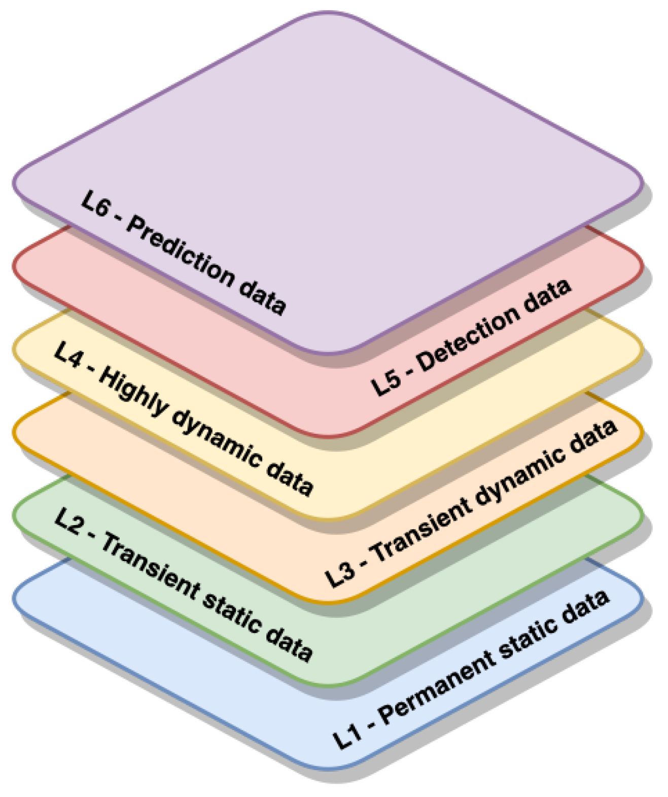
and was organized in a four-layer structure that stores data with different levels of dynamicity:

• Permanent static data (e.g., road topography);
• Transient static data (e.g., position of traffic signs);
• Transient dynamic data (e.g., temporary speed limits due to roadworks);
• Highly dynamic data (e.g., other ITS-Ss information).

Research on the LDM can be divided into two main branches: research that built on top of the existing standardized structure, and research that did not. Regarding the former, the most notable works are from Hideki Shimada et al. [7], who followed ETSI guidelines to implement the LDM; Nicole El Zoghby et al. [8], who increased the Field of View (FoV) of communicating vehicles by fusing the fourth layer of shared LDMs; Fatima Almheiri et al. [9], who paved the way to higher levels of AD by extending the LDM with additional layers for information gathered externally; Carlos Mateo Risma Carletti et al. [10], who extended the standard LDM with their Platoon LDM, a shared database system that efficiently manages data within autonomous vehicle platoons, reducing redundancy and computational demands. A greater amount of research has instead focused on modifying and redefining the standardized LDM. The main works include Bart Netten et al. [11], who saw ETSI LDM as primarily meant for in-vehicle applications and proposed DynaMap, a LDM specialised for roadside applications; Mikel García et al. [12], who presented a data model for the LDM which is both scalable and flexible using a Neo4j graph database and OpenLABEL as a common data format; Maike Scholtes et al. [13], who developed a six-layer LDM that increases the granularity of the information and enriches its contents; Kun Jiang et al. [14], who proposed a seven-layer structure that solves the lane-level map model and route planning problems.

The LDM represents a great tool to efficiently store the data needed and collected by an AV, but it is limited to remaining local to the ITS it runs on. To overcome this issue, the idea is to combine it with CP, allowing ITSs to share data and combine their respective local information. CP is defined by ETSI in [15] as

“the concept of actively exchanging locally perceived objects between different ITS-Ss by means of V2X communication technology”

By means of CP, ITS-Ss can share information to be merged in their LDM, resulting in wider FoVs and more accurate detection, amongst other things, without the need for prohibitively expensive sensor systems.

Significant contributions to CP research include the following: Seong-Woo Kim et al. [16,17,18], who created a framework to extend perception beyond line-of-sight, a cooperative driving system using CP, and methods for improving AD safety and smoothness; Pierre Merdiganc et al. [19], who integrated perception and vehicle-to-pedestrian communication to enhance Vulnerable Road Users’ (VRUs) safety; Aaron Miller et al. [20], who developed a perception and localization system allowing vehicles with basic sensors to leverage data from those with advanced sensors, thus elevating AD capabilities; Xiaboo Chen et al. [21,22], who proposed a recursive Bayesian framework for more reliable cooperative tracking, and a robust framework for multi-vehicle tracking under inaccurate self-localization; Adamey et al. [23], who introduced a method for collaborative vehicle tracking in mixed-traffic settings; Francesco Biral et al. [24], who demonstrated how the SAFE STRIP EU project technology aids in deploying the LDM for Cooperative ITS safety applications; and Stefano Masi et al. [25], who developed a cooperative roadside vision system to enhance the perception capabilities of an AV; Sumbal Malik et al. [26], who highlight the need for advanced CP to overcome challenges in achieving level 5 AD; Tania Cerquitelli et al. [27], who discussed in a special issue the integration of machine learning and artificial intelligence technologies to empower network communication, analysing how computer networks can become smarter; Andrea Piazzoni et al. [28], who discuss how to model CP errors in AD, focusing on the impact of occlusion on safety and how CP may address it; Zhiying Song et al. [29], who presented a framework for evaluating CP in connected AVs, emphasizing the importance of CP in increasing vehicle awareness beyond sensor FoV; Mao Shan et al. [30], who introduced a novel framework for enhancing CP in Connected AVs by probabilistically fusing V2X data, improving perception range and decision-making in complex environments.

The VeDi 2025 project (Mise—Ministero dello Svilippo Economico, actually Ministero delle imprese e del, made in Italy) used V2X communication for manoeuvre negotiation between connected and Automated Vehicles. Amongst the enabling technologies, VeDi 2025 studied Local Dynamic Maps as a means to efficiently store perception data within the vehicle and then make those data available to applications. Given the need for Automated Vehicles to improve their awareness horizon, CPMs were used to enhance vehicle perception beyond the sensors also considering that not all road users (e.g., vehicles, pedestrians) are equipped with V2X communication. Using CPM, as demonstrated, e.g., in 5G CARMEN, the ego vehicle can be aware of the surrounding environment by means of its own sensors and shared sensors’ data.

The purpose of this study, carried out within the VeDi 2025 project, is to add two layers to the standardized LDM, and develop efficient and accurate algorithms designed to enhance AD by exploiting the LDM coupled with CP. To achieve this, we designed, implemented, and tested a six-layer LDM that extends the standardized four-layer structure. The fifth layer maps detected non-connected entities (e.g., VRUs), whilst the sixth maps the predicted future actions of such detected entities. The LDM is implemented as a Neo4j graph database with a custom Application Programming Interface (API), developed with the Python language, that manages it and implements the algorithms. Finally, the implementation is tested on real-world data which we collected with a prototype vehicle from Centro Ricerche FIAT (CRF) in the urban, suburban, and highway scenarios of the Trento area, Italy. Aside from this brief introduction, the rest of the article is organized as follows: Section 2 describes with sufficient detail the design, the implementation, and the testing framework of the developed multi-layered LDM; Section 3 reports and interprets the results obtained from the conducted tests; Section 4 discusses the developed solution analysing the obtained results; Section 5 summarizes the main results, and discusses the possible future works, concluding the article. The abbreviations used in this paper are listed in the Abbreviations section at the end of the paper, just above the appendices.

2. Materials and Methods

2.1. Design

This section describes the design of the developed LDM by discussing: the overall structure, the digital maps utilized, the collected real-world data, and the developed algorithms.

2.1.1. Structure

The developed LDM has the following six-layer structure (Figure 1).

In which each layer holds:

• Termanent static data typically provided by a map data supplier (e.g., road topography);
• Transient static data obtained during operation (e.g., position of traffic lights);
• Transient dynamic data (e.g., traffic light signal phase),
• Highly dynamic data (e.g., other ITS-Ss information);
• Detection data (e.g., the position of a detected legacy vehicle);
• Prediction data (e.g., the predicted future position of a detected legacy vehicle).

2.1.2. Digital Maps

The foundational two layers of the LDM consist of static data sourced from a digital map provider. OpenStreetMap (OSM) was selected for this purpose because of its robust community support, high-quality maps, and its compatibility with Python.

As detailed in [31], OSM maps are characterized by three primary elements: nodes, ways, and relations. Nodes represent specific points of interest (such as traffic lights), ways are sequences of nodes (like a road), and relations are combinations of nodes, ways, and other relations (an example being a park). Additionally, each of these elements can be further defined using tags.

2.1.3. Collected Real-World Data

We collected the real-world data with a prototype AV from CRF Trento Branch in different scenarios covering the urban, suburban, and highway areas of Trento, depicted in Figure 2. They were chosen based on features that would test the algorithms and performance of the LDM on different levels of difficulty.

Urban Scenario

The urban scenario, shown in Figure 2a, has a high number of tightly packed detected entities, mainly pedestrians, but a road network with only 90° turns. Tracking pedestrians is harder than tracking vehicles due to their smaller size, the limitations of the camera to track grouped targets, and the uncertainties associated with the prediction of their trajectories. Moreover, its OSM map has a high density of nodes and ways. These features heavily test the capability of the match detection Algorithm 1 and of the entity positioning Algorithm A5.

Algorithm 1 Match Detection

1: function match_detection($m_k,P_k,m\_r_{k-1},P\_r_{k-1},dt$)                    ▹ k omitted for clarity 2:      for $i=0..length\left(m\right)$ do 3:            for $j=0..length(m\_r)$ do 4:                  $m\_r_j,P\_r_j\leftarrow predict\_state(m\_r_{{k-1}_j},P\_r_{{k-1}_j},dt)$ 5:                  $m\_f_{ij},P\_f_{ij}\leftarrow update(m\_r_j,P\_r_j,m_i,P_i)$ 6:                  $cos{t}_{ij}\leftarrow -log\_likelihood(m_i,m\_f_{ij},P_i)$ 7:            $-log\_likelihood(m\_r_j,m\_f_{ij},P\_r_j)$ 8:            end for 9:      end for 10:     $best\_matches\leftarrow HungarianAlgorithm\left(cost\right)$ 11:     $m\_out,P\_out\leftarrow unique(m\_f,P\_f,m,P,m\_r,P\_r,best\_matches)$ 12:     return $m\_out,P\_out$ 13: end function

where m and $m_r$ are lists of local (i.e., from the ego vehicle) and received state estimates, P and $P_r$ are lists of local and received state estimated covariances, and $dt$ is the prediction time step.

Suburban Scenario

The suburban scenario, shown in Figure 2b, has a road network with some slight turns to exit the main road, but few sparse detected entities. In addition, its OSM map was the only one to contain roundabouts. These features heavily test the capability of the action prediction Algorithm A3 and of the entity positioning Algorithm A5.

Highway Scenario

The highway scenario, shown in Figure 2c, has a high number of sparse detected entities, mainly vehicles, and the road network only has slight turns to exit the highway. Its OSM map is relatively simple, but contains roads that overlap at different altitudes. These features heavily test the match detection Algorithm 1, the action prediction Algorithm A3, and the entity positioning Algorithm A5.

The data comprise information about the ego vehicle and the entities it detected, and comes from sensors such as a Global Navigation Satellite System (GNSS) and cameras. GNSS is the standard generic term for satellite navigation systems that provide geo-spatial positioning with global coverage. Examples are Europe’s Galileo, the USA’s GPS, Russia’s GLONASS, and China’s BeiDou. These data are pre-processed with MATLAB before being used to make it more usable from Python. Processing includes reordering of the data and Geodetic coordinates conversion to Earth-Centered Earth-Fixed (ECEF), amongst other things. A complete description of the collected data can be found in Appendix A.

It is important to specify that some drift in the filtering system, caused by the challenging environmental conditions (e.g., mountains and tall buildings) in which we collected the data, resulted in higher uncertainties than expected. Moreover, due to difficulties in collecting data with more than one vehicle, this dataset does not include proper CP data, only data coming from the ego vehicle. However, we overcame the absence of proper CP data using past data present in the database, and the high uncertainties proved to be useful in developing robust algorithms. Further details on these aspects are provided in the following sections.

2.1.4. Algorithms

Hereafter, a brief explanation of the five algorithms developed to handle detected entities is presented. They predict their next state and action, unequivocally match and position them on the map, and avoid possible collisions.

Predict State

This algorithm predicts the next state of an entity using the prediction step of an Extended Kalman Filter (EKF) [33] which uses an augmented quasi-constant turn dynamical model which also estimates the longitudinal acceleration and the yaw rate; the details of the dynamical model can be found in Appendix B.1.

Match Detection

This algorithm, which has been adapted from the one found in [20], unequivocally matches detected entities between different time instants and data sources (i.e., AVs sharing CP data). Hereafter, the steps the algorithm performs to achieve this are presented.

• It takes as input two lists of detected entities (i.e., state estimates and state estimated covariances); one for the entities detected by the ego vehicle and one for every other detected entity that needs to be matched (e.g., past data present in the database, received data from other vehicles).
• Then, it makes sure to predict the received entities at the current time step using the Predict State Algorithm 2.
• Afterwards, it fuses those estimates in pairs via the update step of a Kalman Filter (KF) [33] which uses a linear measurement model; the details of the measurement model can be found in Appendix B.2. The result is a matrix of fused pairs of estimates.
• Then, it computes a cost matrix by calculating the cost of each pair using the logarithmic likelihood.
• Lastly, it determines the best matches using the Hungarian Algorithm [34] on that cost matrix. If the cost of the best match is negative, the two estimates are considered to be from the same entity; otherwise, they are not not.

Algorithm 2 Predict State

1: function predict_state($m_{k-1},P_{k-1},dt$) 2:     $m_k,P_k\leftarrow EKF\_predict(m_{k-1},P_{k-1},dt)$ 3:     return $m_k,P_k$ 4: end function

where $m_k$ is the state estimate at time step k, $P_k$ is the state estimated covariance at time step k, and $dt$ is the prediction time step.

Action Prediction

Before explaining this algorithm, we first need to understand the basic concept that supports it. It is built upon the concept of motion primitives and action selection [35]. Motion primitives are obtained from the solution of an Optimal Control Problem (OCP) that minimises the longitudinal jerk, which is known to model human-like manoeuvres [35,36] and also used to predict driver intention [37]. Their solution yields longitudinal trajectories for space, velocity, acceleration, and jerk. The motion primitives are analytical polynomials parameterised with initial and final states and few parameters associated with manoeuvre urgency or completion time. Thus, they represent a family of manoeuvres and in this work we used stop and pass manoeuvres At each time instant, multiple motion primitives can be generated. To choose one (i.e., action selection), we used the minimal intervention principle (i.e., Human-Directed jerk) which prioritises the solution with the lowest initial jerk. The complete description of the motion primitives and action selection can be found in Appendix B.3.

Now that the concept of motion primitives and action selection is clear, we can move on to the Action Prediction algorithm. Due to the size of this algorithm, hereafter, only a summary of its steps is reported; for the full version of the algorithm, please refer to Appendix B.4.

• The input is a list of detected entities along with all the possible actions they could take (e.g., turn left, go straight).
• For each possible action, a good approximation for the final distance $s_f$ is the length of a clothoid that connects the starting point to the point of interest. Combining this information with the initial conditions taken from the data (i.e., $v_0$ and $a_0$) we can compute the stop motion.
• The velocity range can be estimated from $a_0$. If it is positive, the entity is likely to increase its final velocity. If it is negative, the entity is likely to decrease its final velocity. Lastly, if it is zero, we can not make any assumptions about the final velocity. With the estimate of the final velocity, we can heuristically assign a velocity interval based on road regulations and the vehicle’s initial velocity.
• We directly compute the time range from the velocity range and the distance to the point of interest. We can now compute the pass motion.
• The chosen motion is the one with the minimum initial longitudinal jerk.

Using only information on the longitudinal jerk is not enough to distinguish which action would be more likely to be taken (e.g., turn right or go straight might have the same initial longitudinal jerk). Therefore, we need to introduce information on the lateral motion of the vehicle. Instead of complicating the OCP, we introduce a second weighting term—for the action selection—based on the maximum lateral acceleration. A reliable estimate of the lateral acceleration can be achieved by multiplying the longitudinal velocity profile, squared, by the curvature of the clothoid representing the manoeuvre as mentioned earlier. This second weighting factor ensures that the action most likely to be selected is the one that minimizes both the initial longitudinal jerk and the peak lateral acceleration.

Collision Avoidance

Once we obtain the most likely actions the detected entities might take, we can use them to predict possible future collisions with the ego vehicle. Due to the size of this algorithm, hereafter, only a summary of its steps is reported; for a full version of the algorithm, please refer to Appendix B.5.

• Leveraging the fact that the database is a graph, find all map nodes that are an intersection between the ego vehicle and the detected entities’ possible paths. The input to the algorithm is a list composed of these nodes, data on the ego vehicle, and data on the detected entities (e.g., velocity).
• A good approximation of the path length (i.e., $s_f$) can be computed by joining each map node of the path using clothoids. With the path length we can compute the stop motion for all the detected entities involved in the possible collision.
• The velocity and time ranges are computed in the same way as described in the action prediction algorithm. We can now compute the pass motion for each detected entity as well.
• If the best motion primitive (i.e., the one with minimum initial jerk) is a stop motion, then there should be no risk of collision. Instead, if the best motion primitive is a pass motion, that primitive will be saved as a collision primitive.
• We can use the final time of the collision primitive to compute the velocity and time ranges for the ego vehicle and evaluate stop and pass motions to avoid that collision. The choice is once again made using the minimum intervention principle.

Entity Positioning

This algorithm positions an entity in the correct way by using only its absolute position and its Course Over Ground (COG). It was developed to correctly position an entity even in the presence of high uncertainties in the absolute position, when the closest way, in a Euclidean distance sense, may not be the correct one. Due to the size of this algorithm, hereafter, only a summary of its steps is reported; for a full version of the algorithm, please refer to Appendix B.6.

Let us look at Figure 3. The black dots are map nodes, the orange dot is an entity, the dashed green lines represent an imaginary segment between two map nodes (i.e., a way), the dashed purple lines indicate which segment the entity is considered to be on, the orange arrow is the direction of the entity (i.e., its COG). Let us now look at the two nodes of the way the entity is on. The map node the entity is moving towards is considered the node it is on, whilst the other node (i.e., the node it is moving away from) is the node it was on. We can now move on to explaining the main steps of this algorithm.

• If the entity has already been positioned before, the perpendicular distance between the entity and the way it is on is under $8m$, and has not yet crossed the map node it is on, there is no need to reposition the entity.
• If the entity has already been positioned before, the perpendicular distance between the entity and the way it is on is under $8m$, and has crossed the map node it is on, the entity will be re-positioned to an adjacent way which is the one best aligned compared to the vehicle COG.
• Otherwise, the entity needs to be positioned from scratch. To do so, the algorithm retrieves the pair of map nodes that creates a way which is the closest and best aligned to the entity’s movement. To make the two metrics comparable, they have been normalized using the values of $4m$ (i.e., the common width of a street) and ${90}^{\circ }$ (i.e., the maximum angle between the entity COG and the way).

2.2. Implementation

In this section, we describe the implementation of the developed LDM by discussing: the database used to implement the LDM and the API created to interface between the database and the ego vehicle. The code of the developed LDM is available at https://github.com/SebastianoTaddei/Multi-Layered-Local-Dynamic-Map-for-a-Connected-and-Automated-in-Vehicle-System/tree/main (accessed on 16 January 2024).

2.2.1. Database

In terms of implementation, the LDM is essentially a database (DB). Amongst the several types of DBs that exist, the graph DB model was chosen due to its effectiveness in representing real-world scenarios. Neo4j (version 5.10.0.) (https://neo4j.com (accessed on 16 January 2024)), identified as one of the top software options for constructing a graph DB, was our preferred choice due to its demonstrated performance, as noted in [12], and its seamless compatibility with Python.

2.2.2. Interface between Database and Ego vehicle

The API has been developed completely in Python with the main tasks of creating and managing the LDM. It is composed of three main files that handle the requests to the Neo4jDB, the utility functions that to not query the DB, and the processing of incoming data. Without entering the details, let us look at the API block diagram in Figure 4 to better understand how it works.

At the top of Figure 4 we have incoming data which contain information on the ego vehicle (e.g., position and velocity), on the connections (e.g., position of other AVs that share information with the ego vehicle), and on the detected entities (e.g., any entity detected by either the ego vehicle or another connected entity). Afterwards, the map information is loaded (through the osmfunction) based on the ego vehicle position; the map data goes directly into the DB. Before positioning the entities with the entity positioning algorithm, the detection data undergo the process of matching through the function match and the algorithm match detections; after being positioned, these data are saved in the DB as well as going to other stages. In addition, the future state of each detected entity is predicted and saved in the DB. The last stages involve the prediction of the actions for each detected entity using the action prediction algorithm, and the avoidance of collisions by combining the predicted actions, the ego vehicle data, and the predicted future states of the detected entities into the collision avoidance algorithm.

2.3. Test and Validation

This section describes the test setup and the metrics utilized to validate the developed LDM. We tested the LDM in simulation by replaying real-world data logged at a frequency of 0.1 s by a prototype AV from CRF. As such, each step of our simulation corresponds to 0.1 s of real-world time and assumes that to be the real-time threshold. The simulation is run completely in Python.

2.3.1. Testing Hardware

Each test has been run on a 16” MacBook Pro with an M2 Max chip (12-core CPU, 30-core GPU, 32 GB RAM, and 1 TB SSD).

2.3.2. Test Setup

Let us first analyse in detail a couple of frames taken from an output video generated by the simulation to ease the discussion and interpretation of the results that come later on.

Looking at Figure 5, we can see that each frame has the following features:

• A dynamically changing map;
• Each map node is represented as a green dot;
• The ego vehicle is viewed as an orange dot;
• Each detected entity which has been matched is reported as a black dot, which are usually shadowed by the ground truth blue dot;
• The ground truth (i.e., the received measurements at every time step) for each detected entity is reported as a blue dot, which usually shadows the detected entity black dot;
• The purple dashed line indicates the node an entity will go to;
• The blue dashed line indicates the node an entity is going away from;
• The grey dot-dashed line pictures the predicted trajectory of a detected entity;
• The name for each entity is reported in black text;
• The type of predicted action (i.e., type of motion primitive) is reported in magenta text.

Moreover, in case any collision might occur, the trajectories for each involved entity will be drawn in red alongside the type of action (i.e., motion primitive) to prevent it, as can be seen in Figure 6.

2.3.3. Key Performance Indicators

To evaluate the performance of the LDM, several metrics have been devised that are described next.

Matching accuracy measures how accurate the match detection algorithm is, and is computed as

$$\mathit{Matching}\mathit{accuracy}=\frac{\mathit{correct}\mathit{matches}}{\mathit{total}\mathit{matches}}.$$

Processing time allows us to determine whether the LDM is capable of real-time operation or not. It is divided into three Key Performance Indicators (KPIs) to better understand the behaviour of the LDM. The first KPI is the average time took by the LDM to process one step of the simulation composed of M steps over N runs

$${\overline{\mathit{Processing}\mathit{time}}}_{\mathit{one}\mathit{step}}=\frac{{\sum }_N{\sum }_M\mathit{LDM}\mathit{one}\mathit{step}\mathit{processing}\mathit{time}}{MN}.$$

We will report this KPI alongside $3\overline{\sigma }$ (i.e., three times the average standard deviation over N runs) to cover approximately $99.7\%$ of the step times. The second KPI is the average time over N runs

$${\overline{\mathit{Processing}\mathit{time}}}_{\mathit{full}\mathit{sim}}=\frac{{\sum }_N\mathit{LDM}\mathit{full}\mathit{sim}\mathit{processing}\mathit{time}}{N}.$$

The last KPI is the average number of simulation steps that the LDM could not process in real-time over N runs

$$\overline{\mathit{Steps}\mathit{not}\mathit{real}-\mathit{time}}=\frac{{\sum }_N\mathit{steps}\mathit{not}\mathit{real}-\mathit{time}}{N}.$$

Data persistence corresponds to the maximum number of prediction steps the LDM can take when predicting the future state of a detected entity without receiving any new measurement. We computed it as the maximum number of prediction steps the LDM can make before degrading the matching performance

$$\mathit{Data}\mathit{persistence}=\mathit{prediction}\mathit{steps}\mathit{until}\mathit{match}\mathit{fails}.$$

Knowing the size of the prediction step (i.e., 0.1 s in our case), one can easily convert this metric to time and understand for how long the LDM accurately predicts the movement of a detected entity.

Action prediction accuracy measures the accuracy of the action prediction algorithm and is computed as

$$\mathit{Action}\mathit{prediction}\mathit{accuracy}=\frac{\mathit{correct}\mathit{action}\mathit{predictions}}{\mathit{total}\mathit{actions}}.$$

3. Results

The LDM has been tested on the three scenarios described in Section 2.1.3 which cover an urban, a suburban, and a highway area of Trento. Let us analyse the results obtained for each of the KPIs.

3.1. Matching Accuracy

Before looking at the results, we need to disclose how the correct matches are defined and counted. The sensing system of the vehicle is capable of tracking an entity over time. When it first detects an entity, it assigns it a unique identifier (ID) that will be kept constant over time. Unfortunately, whenever the system loses sight of that entity, the unique ID is freed and ready to be used for another entity in a matter of seconds. Even though this prevents us from using that ID as an absolute ground truth, we can exploit that time window. To overcome this limitation, we devised the following strategy to identify correct matches between simulation steps.

• The match is considered correctif the IDs are equal.
• The match is considered wrong if the IDs are different and an entity with the an equal ID was available to be matched.
• If the IDs are different, but there was no entity with that ID to be matched, the match is considered correct but is counted separately as maybe since we can not be certain of its correctness.
• Any entity that was not matched (i.e., identified as new entity) is considered correct but is reported separately as unmatched.

The results obtained for each scenario are reported in

Table 1. Matching accuracy.

Scenario	Total	Correct	Maybe	Unmatched	Wrong	Accuracy
Urban	4010	3159	114	147	590	$\approx 85\%$
Suburban	1001	928	13	15	45	$\approx 96\%$
Highway	4201	3821	32	56	292	$\approx 93\%$
Overall	9212	7908	159	927	218	$\approx 90\%$

.

The reason the scenarios have different accuracy is twofold. The first reason is the type of entities and their density. The urban scenario is the most challenging one due to the presence of many pedestrians which are harder to predict than vehicles and are often found in tightly packed groups. Instead, the suburban and highway scenarios mostly had sparse vehicles resulting in a higher matching accuracy. The second reason is the number of times there were matches to make. Whilst the urban and highway scenarios had to perform 4010 and 4201 matches, respectively, the suburban one only had to perform 1001. Moreover, these matches where “ideal” in the sense that this scenario mostly saw one entity at a time. These reasons combined allowed the suburban scenario to obtain the highest matching accuracy overall.

3.2. Processing Time

To measure the processing time, we ran the simulation $N=100$ times for each scenario with a time step of 0.1 s. In particular, the urban scenario was run for 162.5 s resulting in $M=1625$ time steps; the suburban scenario was run for 200 s resulting in $M=2000$ time steps; the highway scenario was run for 200 s resulting in $M=2000$ time steps. The results can be found in

Table 2. Processing time (PT) with a time step of 0.1 s and real-time threshold of 0.1 s.

Scenario	${\overline{\mathit{PT}}}_{\mathit{one}\mathit{step}}+3\overline{\mathit{\sigma }}$	${\overline{\mathit{PT}}}_{\mathit{full}\mathit{sim}}$	$\overline{\mathit{Steps}>0.1\mathbf{s}}$
Urban	0.011 s + 0.045 s < 0.1 s	18.525 s	8
Suburban	0.005 s + 0.021 s < 0.1 s	10.560 s	2
Highway	0.010 s + 0.036 s < 0.1 s	19.146 s	7
Average	$0.008\mathrm{s}+0.035\mathrm{s}<0.1\mathrm{s}$	$15.914\mathrm{s}$	6

.

Let us focus on the second column of Table 2. This column reports the average processing time for one step of the simulation plus three times the average standard deviation, covering approximately $99.7\%$ of the simulation steps. Values below 0.1 s represent real-time capability, whilst values above indicate the opposite. We can clearly see that the LDM is capable of real-time operation under all the considered scenarios. The reasons for the different performances in the scenarios are multiple, but the main two are the density of map nodes and detected entities to match. The urban scenario has the highest density of both map nodes and detected entities, resulting in a higher computational cost. The suburban scenario has the lowest density of both, therefore costing the least computationally speaking. Lastly, the highway scenario has roughly the same amount of detected entities as the urban scenario but fewer map nodes, and are both rather sparse, obtaining processing times slightly better than the urban scenario. The third column of Table 2 emphasizes the real-time capabilities of the LDM by reporting the total average time the LDM took to process the entire simulation. All scenarios are well below the respective total real-world time.

Shifting the focus to the fourth column of Table 2, we can see that there are some instances in which the LDM is not real-time. Whilst these steps could be considered outliers, we must explain them. The reason we believe they are above the real-time threshold are many, such as the communication to the Neo4j database and the slow loading of OSM maps. Whilst using an external DB has its benefits (e.g., modularity, reuse of data from multiple clients), it comes with inevitable communication delays. This forces us to reduce calls to the DB to a minimum and maximize the data sent in each call. However, since the amount of data managed by the local LDM is low, the communication delay ends up dominating the processing time. In addition, the procedure we implemented to quickly ingest the OSM maps in the Neo4j DB, is not as optimized as one we could make with an embedded DB. Therefore, to verify these assumptions we implemented a preliminary version of the LDM using the NetworkX Python package [38] instead of Neo4j to manage the graph DB directly in Python, removing calls to the external DB. From the preliminary results shown in

Table 3. Preliminary processing time (PT) with a time step of 0.1 s and real-time threshold of 0.1 s.

Scenario	${\overline{\mathit{PT}}}_{\mathit{one}\mathit{step}}+3\overline{\mathit{\sigma }}$	${\overline{\mathit{PT}}}_{\mathit{full}\mathit{sim}}$	$\overline{\mathit{Steps}>0.1\mathbf{s}}$
Urban	0.009 s + 0.033 s < 0.1 s	14.539 s	0
Suburban	0.002 s + 0.006 s < 0.1s	3.152 s	0
Highway	0.005 s + 0.024 s < 0.1 s	10.381 s	2
Average	$0.005\mathrm{s}+0.024\mathrm{s}<0.1\mathrm{s}$	$9.357\mathrm{s}$	1

, we can see that using an embedded DB, and a better map ingestion procedure, almost entirely removes the steps that were above the real-time threshold of 0.1 s, indicating that those two aspects were indeed amongst the main reasons for the rare drop in performance of the LDM.

3.3. Data Persistence

By default, the LDM can predict the next state of a detected entity for 2 time steps, after which it deletes that entry from the LDM. By changing the maximum number of allowed prediction steps, we can determine for how long the LDM can predict the next state of an entity by noticing when the matching performance worsens (i.e., when the number of wrong matches increases).

Let us look at

Table 4. Data persistence.

Scenario	Persistence	Total	Correct	Maybe	Wrong	Unmatched
Urban	6	$-4$	$+23$	$-12$	$+0$	$-15$
Suburban	5	$+2$	$+1$	$+0$	$+0$	$+1$
Highway	2	$+0$	$+0$	$+0$	$+0$	$+0$
Average	4	-	-	-	-	-

, which reports the differences between the default performance (i.e., obtained with maximum 2 prediction steps) and the performance obtained by increasing the number of prediction steps, as well as the persistence metric. Remembering that the prediction step is fixed at 0.1 s, we can easily convert the persistence metric to time. We can see that in the urban scenario, the LDM was able to predict the movement of an entity for $6\mathit{steps}=0.6\mathrm{s}$, improving the number of correct matches whilst reducing the uncertainty in the maybe and unmatched matches. In the suburban scenario, it was able to predict the movement for $5\mathit{steps}=0.5\mathrm{s}$, also improving its performance but only marginally. Instead, the highway scenario was unable to improve over the default maximum prediction steps of $2\mathit{steps}=0.2\mathrm{s}$. The reason the LDM could not increase the persistence over the default value is due to the difficulty of predicting the movement of an entity at higher speeds. In fact, the faster a vehicle goes, the more distance it will cover in the same amount of time, making it harder to predict its next state precisely.

3.4. Action Prediction Accuracy

To compute this metric we selected sub-portions of the three scenarios and manually counted the times the LDM was able to correctly predict the next action of an entity. The results for each scenario are reported in

Table 5. Action prediction accuracy.

Scenario	Total	Correct	Accuracy
Urban	101	92	$\approx 91\%$
Suburban	91	83	$\approx 91\%$
Highway	36	27	$\approx 75\%$
Overall	228	202	$\approx 89\%$

, whilst the selected portion of each scenario is reported in Figure 7.

The findings indicate that the LDM is more effective in predicting actions near T-junctions as compared to bifurcations. This outcome aligns with expectations, as it is generally simpler to predict whether an entity will proceed straight or make a ${90}^{\circ }$ turn, rather than determining if it will make a slight right turn to leave a highway.

3.5. Collision Avoidance

Even though we were unable to gather proper CP data to thoroughly test the collision avoidance algorithm, there was an example in our test data which clearly shows its potential and is reported in Figure 6. Note that this occurrence was only possible thanks to high uncertainty in the position of a detected entity which forced the LDM to position it on the wrong way, while it should have been in front of the ego vehicle instead.

Looking at Figure 6 we can see the ego vehicle and a legacy vehicle approaching the same junction. The LDM correctly identifies the junction node as a possible collision point, draws the trajectories of all entities involved and suggests the ego vehicle the motion primitive to avoid that collision. Whilst this example does not validate the algorithm, it shows its capabilities and potential.

4. Discussion

In this section, we discuss the the results we reported in Section 3 that show, via the KPIs, the effectiveness of using the LDM as a DB for both data generated by the AV and incoming data from other entities.

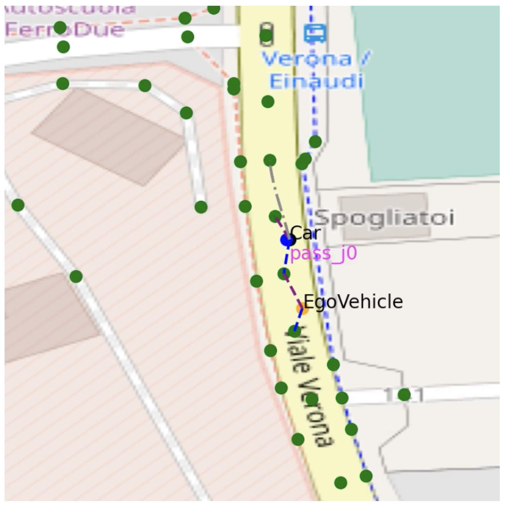
Regarding the matching accuracy, whose results are reported in Table 1, we obtained an overall accuracy of $\approx 90\%$ across the scenarios, meaning we could correctly match entities coming from different (simulated with past DB data) sources. This result is significant on its own, and is especially so after considering the challenging conditions in which we collected the data. As it is often the case with GNSS-related data, the uncertainty in the received measurements is heavily dependent on environmental aspects. Having conducted the tests in Trento, an Italian city with relatively high buildings and surrounded by mountains, we knew in advance that the resulting measurements would not have had the ideal performance of the sensor system. This resulted in position errors of at least 2 m, which are especially relevant for the tight urban area of Trento. Given that the incoming data of the sensor system was already filtered, and we were working in post-processing, we decided to take it “as is”, as this would be the case for incoming measurements received via CP. However, once we deploy our solution on the prototype vehicle and use it online, we will consider the use of additional advanced estimation techniques, such as the robust lateral velocity estimator developed by Mauro Da Lio et al. in [39], to reduce the uncertainty of the GNSS system.

Moving on to the processing time Table 2, we obtained an average computation time per step of only 0.008 s + 0.035 s < 0.1 s, less than half of our real-time threshold. However, we did have six steps which were above the 0.1 s threshold. After developing a prototype of our LDM using NetworkX instead of Neo4j, whose results are reported in Table 3, we were able to say that the communication between the external Neo4j DB and the loading of OSM maps were key factors in making those steps surpass the real-time threshold. While developing the prototype with NetworkX, we also identified the main weakness of Neo4j. Although Neo4j is incredibility fast with large graphs (i.e., millions of nodes and edges), the delay it takes to send a request to the database is not worth it for smaller graphs like ours (i.e., tens of thousands of nodes and edges). Therefore, we came to the conclusion that a graph DB managed directly in Python, such as NetworkX, better suits the needs of the small graph we keep local to the AV. On the other hand, Neo4j would make more sense to be deployed on the infrastructure side; if the graph size was likely to be far greater, the communication delay would be less noticeable, and the scalability of Neo4j would immediately show its benefits. Lastly, changing to a DB managed directly inside the API would allow us to convert the codebase to C++ and use the igraph package [40], which would increase our performance by at least one order of magnitude.

The data persistence KPI, whose results are reported in Table 4, tells us the maximum number of prediction steps the LDM can take when predicting the future state of a detected entity without receiving any new measurement. Since the prediction step corresponds to 0.1 s, we can conclude that on average the LDM was able to predict the movement of detected entities for $4\mathit{steps}=0.4\mathrm{s}$ across all scenarios. This is crucial as it enables the LDM to not lose “sight” of an entity even if it momentarily disappears behind a blind corner or a bus. Although the prediction window is not wide, $0.4\mathrm{s}$ is enough to fill in the blanks that may emerge from communication delays/interruptions or temporary occlusions of entities, just to name a few. Improving the positioning of the ego vehicle and/or of detected entities, for example, using additional advanced estimation techniques like the one mentioned a few lines above [39], will undoubtedly improve the data persistence capabilities as well.

Lastly, the action prediction accuracy, whose results are reported in Table 5, shows us how accurate the LDM is in predicting where a detected entity will go next. With an overall accuracy of $\approx 89\%$, we can confidently say we know where an entity will be most of the time. This is also an area that would benefit from additional advance estimation techniques, just like with data persistence. Moreover, at the moment, we are focusing only on predicting actions at each time step, but we could try to use multiple past predictions to have a more reliable estimate after some time steps.

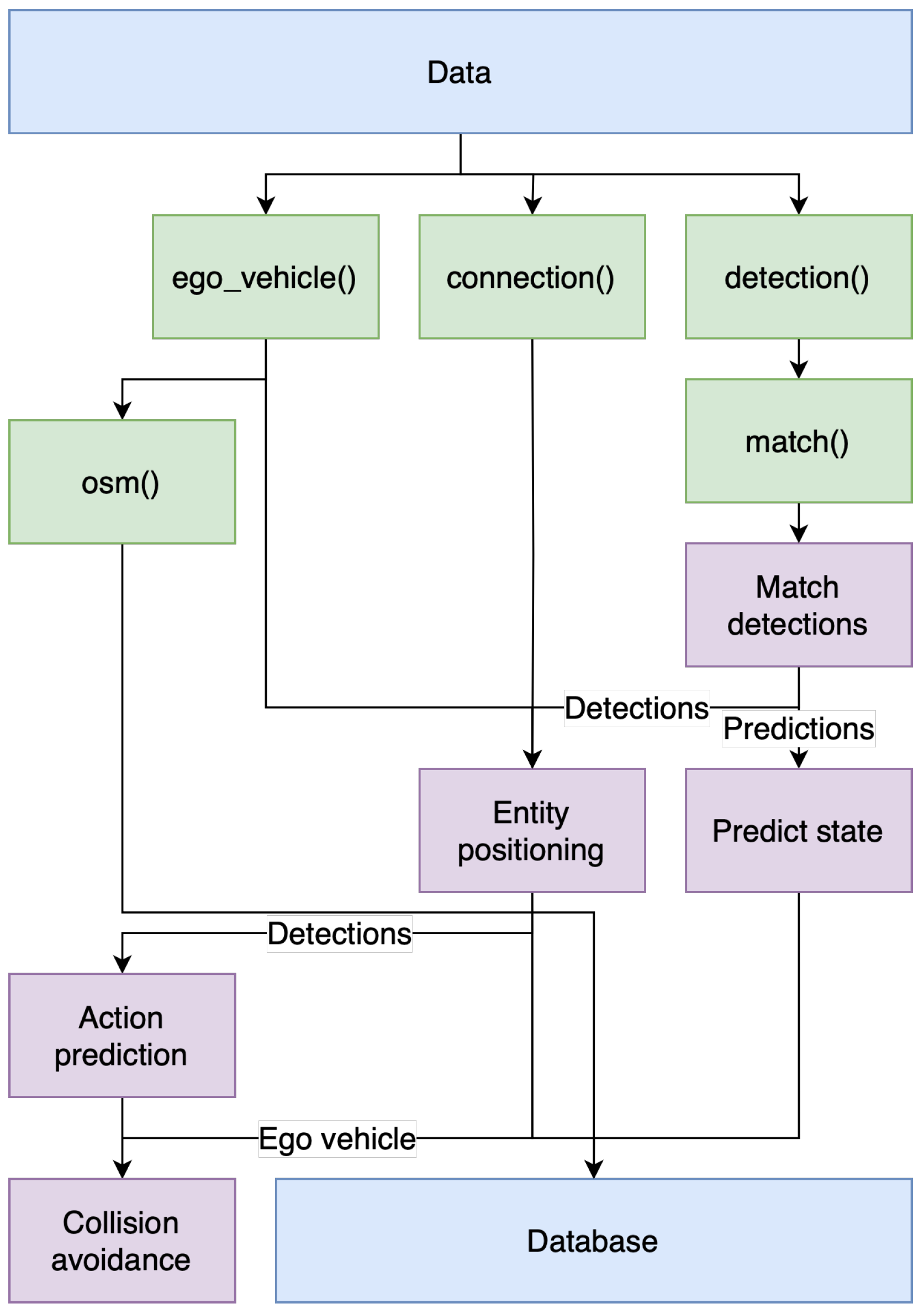
All in all, we can confidently say that the ability to easily handle environmental and detection data, be they from the ego vehicle or through CP, allowed us to quickly develop algorithms that support the development of AD. We have not talked about the collision prediction algorithm as we did not have enough data, but that is just one of the many algorithms we can develop by building on top of the readily available data stored in the LDM. In fact, thanks to entity positioning, match detection, data persistence, and action prediction algorithms, we could easily develop the collision avoidance algorithm with just some additional logic and a few lines of code. That is why we are planning to embed our LDM in our motion planning framework for at-limit handling of racing vehicles [41], to have a separate application that can take the burden of analysing the environment of interest and serve vital information quickly, reliably, and only when needed (e.g., an incoming collision or the next action of an opponent on the racetrack).

5. Conclusions

In this paper, we developed and tested a multi-layered Local Dynamic Map (LDM) coupled with Cooperative Perception (CP) with the aim of developing robust and accurate algorithms suited for Automated Driving (AD). The developed solution is shown to be capable of matching detected entities with an average accuracy of $\approx 90\%$, predicting the next state of an entity for an average time of $\approx 0.4\mathrm{s}$ without receiving any new measurement, and predicting the action of an entity with an average accuracy of $\approx 89\%$. Moreover, it is capable of performing these tasks in real time. The LDM coupled with CP has proven to be an effective tool to incorporate the incoming data and augment its capabilities beyond the single received measurements. The developed solution has the ability to enhance a state-of-the-art sensor system, facilitating the creation of robust and accurate algorithms that contribute to the development of AD.

In conclusion, we will focus our future research on the following:

• Enhancing the matching algorithm by varying parameters based on the type of entity detected;
• Converting the LDM to C++ and using the igraph package [40] to manage the graph database directly in the API;
• Using the LDM to augment the capabilities of our motion planning framework for at-limit handling of racing vehicles [41];
• Using additional advanced estimation techniques [39] to increase the accuracy of the GNSS system;
• Deploying the developed solution on the prototype Automated Vehicle from CRF Trento Branch and testing it online.

References

1. Transport Statistics at Regional Level. Available online: https://ec.europa.ehttps://ec.europa.eu/eurostat/statistics-explained/index.php?title=Transport_statistics_at_regional_level#Road_transport_and_accidents (accessed on 1 November 2023).
2. Waymo. Available online: https://waymo.com/ (accessed on 10 February 2022).
3. Andreone, L.; Brignolo, R.; Damiani, S.; Sommariva, F.; Vivo, G.; Marco, S. SAFESPOT Final Report; Technical Report; 2010. Available online: http://www.safespot-eu.org/documents/D8.1.1_Final_Report_-_Public_v1.0.pdf (accessed on 26 January 2022).
4. Kompfner, P.; Castermans, J. CVIS Final Activity Report; Technical Report; 2010. Available online: https://trimis.ec.europa.eu/sites/default/files/project/documents/20120713_132648_5935_DEL_CVIS_1.3_FinalActivityReport_PartII_PublishableSummary_V1.0.pdf (accessed on 26 January 2022).
5. ETSI TR 102 863 V1.1.1; Intelligent Transport Systems (ITS); Vehicular Communications; Basic Set of Applications; Local Dynamic Map (LDM); Rationale for and Guidance on Standardization. European Telecommunications Standards Institute (ETSI), 2011. Available online: https://www.etsi.org/deliver/etsi_tr/102800_102899/102863/01.01.01_60/tr_102863v010101p.pdf (accessed on 24 January 2022).
6. ETSI EN 302 895 V1.1.1; Intelligent Transport Systems (ITS); Vehicular Communications; Basic Set of Applications; Local Dynamic Map (LDM). European Telecommunications Standards Institute (ETSI), 2014. Available online: https://www.etsi.org/deliver/etsi_en/302800_302899/302895/01.01.01_60/en_302895v010101p.pdf (accessed on 24 January 2022).
7. Shimada, H.; Yamaguchi, A.; Takada, H.; Sato, K. Implementation and Evaluation of Local Dynamic Map in Safety Driving Systems. J. Transp. Technol. 2015, 5, 102–112. [Google Scholar] [CrossRef]
8. Zoghby, N.E.; Cherfaoui, V.; Denoeux, T. Evidential distributed dynamic map for cooperative perception in VANets. In Proceedings of the 2014 IEEE Intelligent Vehicles Symposium Proceedings, Dearborn, MI, USA, 8–11 June 2014; pp. 1421–1426. [Google Scholar] [CrossRef]
9. Almheiri, F.; Alyileili, M.; Alneyadi, R.; Alahbabi, B.; Khan, M.; El-Sayed, H. evolved Local Dynamic Map (eLDM) for Vehicles of Future. In Proceedings of the 2021 6th International Conference on Computational Intelligence and Applications (ICCIA), Xiamen, China, 11–13 June 2021; pp. 292–297. [Google Scholar] [CrossRef]
10. Carletti, C.M.R.; Casetti, C.; Härri, J.; Risso, F. Platoon-Local Dynamic Map: Micro cloud support for platooning cooperative perception. In Proceedings of the 2023 19th International Conference on Wireless and Mobile Computing, Networking and Communications (WiMob), Montreal, QC, Canada, 21–23 June 2023; pp. 405–410. [Google Scholar] [CrossRef]
11. Netten, B.D.; Kester, L.J.H.M.; Wedemeijer, H.; Passchier, I.; Driessen, B. Dynamap: A Dynamic Map for Road Side Its Stations; Intelligent Transportation Society of America: Washington, DC, USA, 2013. [Google Scholar]
12. García, M.; Urbieta, I.; Nieto, M.; González de Mendibil, J.; Otaegui, O. iLDM: An Interoperable Graph-Based Local Dynamic Map. Vehicles 2022, 4, 42–59. [Google Scholar] [CrossRef]
13. Scholtes, M.; Westhofen, L.; Turner, L.R.; Lotto, K.; Schuldes, M.; Weber, H.; Wagener, N.; Neurohr, C.; Bollmann, M.H.; Kortke, F.; et al. 6-Layer Model for a Structured Description and Categorization of Urban Traffic and Environment. IEEE Access 2021, 9, 59131–59147. [Google Scholar] [CrossRef]
14. Jiang, K.; Yang, D.; Liu, C.; Zhang, T.; Xiao, Z. A Flexible Multi-Layer Map Model Designed for Lane-Level Route Planning in Autonomous Vehicles. Engineering 2019, 5, 305–318. [Google Scholar] [CrossRef]
15. ETSI TR 103 562 V2.1.1; Intelligent Transport Systems (ITS); Vehicular Communications; Basic Set of Applications; Analysis of the Collective Perception Service (CPS); Release 2. European Telecommunications Standards Institute (ETSI), 2019. Available online: https://www.etsi.org/deliver/etsi_tr/103500_103599/103562/02.01.01_60/tr_103562v020101p.pdf (accessed on 26 January 2022).
16. Kim, S.W.; Chong, Z.J.; Qin, B.; Shen, X.; Cheng, Z.; Liu, W.; Ang, M.H. Cooperative perception for autonomous vehicle control on the road: Motivation and experimental results. In Proceedings of the 2013 IEEE/RSJ International Conference on Intelligent Robots and Systems, Tokyo, Japan, 3–7 November 2013; pp. 5059–5066. [Google Scholar] [CrossRef]
17. Kim, S.W.; Liu, W.; Ang, M.H.; Frazzoli, E.; Rus, D. The Impact of Cooperative Perception on Decision Making and Planning of Autonomous Vehicles. IEEE Intell. Transp. Syst. Mag. 2015, 7, 39–50. [Google Scholar] [CrossRef]
18. Kim, S.W.; Qin, B.; Chong, Z.J.; Shen, X.; Liu, W.; Ang, M.H.; Frazzoli, E.; Rus, D. Multivehicle Cooperative Driving Using Cooperative Perception: Design and Experimental Validation. IEEE Trans. Intell. Transp. Syst. 2015, 16, 663–680. [Google Scholar] [CrossRef]
19. Merdrignac, P.; Shagdar, O.; Nashashibi, F. Fusion of Perception and V2P Communication Systems for the Safety of Vulnerable Road Users. IEEE Trans. Intell. Transp. Syst. 2017, 18, 1740–1751. [Google Scholar] [CrossRef]
20. Miller, A.; Rim, K.; Chopra, P.; Kelkar, P.; Likhachev, M. Cooperative Perception and Localization for Cooperative Driving. In Proceedings of the 2020 IEEE International Conference on Robotics and Automation (ICRA), Paris, France, 31 May–31 August 2020; pp. 1256–1262. [Google Scholar] [CrossRef]
21. Chen, X.; Ji, J.; Wang, Y. Robust Cooperative Multi-Vehicle Tracking with Inaccurate Self-Localization Based on On-Board Sensors and Inter-Vehicle Communication. Sensors 2020, 20, 3212. [Google Scholar] [CrossRef] [PubMed]
22. Chen, X.; Wang, Y.; Chen, L.; Ji, J. Multi-Vehicle Cooperative Target Tracking with Time-Varying Localization Uncertainty via Recursive Variational Bayesian Inference. Sensors 2020, 20, 6487. [Google Scholar] [CrossRef]
23. Adamey, E.; Ozbilgin, G.; Ozguner, U. Collaborative Vehicle Tracking in Mixed-Traffic Environments: Scaled-Down Tests Using SimVille; SAE Technical Paper 2015-01-0282; SAE International: Warrendale, PA, USA, 2015. [Google Scholar] [CrossRef]
24. Biral, F.; Valenti, G.; Bertolazzi, E.; Steccanella, A. Cooperative Safety Applications for C-ITS Equipped and Non-equipped Vehicles Supported by an Extended Local Dynamic Map built on SAFE STRIP Technology. In Proceedings of the 2019 15th International Conference on Distributed Computing in Sensor Systems (DCOSS), Santorini, Greece, 29–31 May 2019; pp. 733–740. [Google Scholar] [CrossRef]
25. Masi, S.; Xu, P.; Bonnifait, P.; Ieng, S. Augmented Perception with Cooperative Roadside Vision Systems for Autonomous Driving in Complex Scenarios. In Proceedings of the 2021 IEEE International Intelligent Transportation Systems Conference (ITSC), Indianapolis, IN, USA, 19–22 September 2021; pp. 1140–1146. [Google Scholar] [CrossRef]
26. Malik, S.; Khan, M.J.; Khan, M.A.; El-Sayed, H. Collaborative Perception—The Missing Piece in Realizing Fully Autonomous Driving. Sensors 2023, 23, 7854. [Google Scholar] [CrossRef]
27. Cerquitelli, T.; Meo, M.; Curado, M.; Skorin-Kapov, L.; Tsiropoulou, E.E. Machine learning empowered computer networks. Comput. Netw. 2023, 230, 109807. [Google Scholar] [CrossRef]
28. Piazzoni, A.; Cherian, J.; Vijay, R.; Chau, L.P.; Dauwels, J. CoPEM: Cooperative Perception Error Models for Autonomous Driving. In Proceedings of the 2022 IEEE 25th International Conference on Intelligent Transportation Systems (ITSC), Macau, China, 8–12 October 2022; pp. 3934–3939. [Google Scholar] [CrossRef]
29. Song, Z.; Wen, F.; Zhang, H.; Li, J. A Cooperative Perception System Robust to Localization Errors. In Proceedings of the 2023 IEEE Intelligent Vehicles Symposium (IV), Anchorage, AK, USA, 4–7 June 2023; pp. 1–6. [Google Scholar] [CrossRef]
30. Shan, M.; Narula, K.; Worrall, S.; Wong, Y.F.; Stephany Berrio Perez, J.; Gray, P.; Nebot, E. A Novel Probabilistic V2X Data Fusion Framework for Cooperative Perception. In Proceedings of the 2022 IEEE 25th International Conference on Intelligent Transportation Systems (ITSC), Macau, China, 8–12 October 2022; pp. 2013–2020. [Google Scholar] [CrossRef]
31. Elements—OpenStreetMap. Wiki. Available online: https://wiki.openstreetmap.org/wiki/Elements (accessed on 11 April 2022).
32. OpenStreetMap. Available online: https://www.openstreetmap.org/ (accessed on 16 February 2022).
33. Hostettler, R.; Särkkä, S. Lecture Notes on Basics of Sensor Fusion. In ELEC-E8740 Class Notes; Uppsala University: Uppsala, Sweden, 2018. [Google Scholar]
34. Hungarian Algorithm, Page Version ID: 1191132310. 2023. Available online: https://en.wikipedia.org/w/index.php?title=Hungarian_algorithm&oldid=1191132310 (accessed on 27 December 2023).
35. Da Lio, M.; Biral, F.; Bertolazzi, E.; Galvani, M.; Bosetti, P.; Windridge, D.; Saroldi, A.; Tango, F. Artificial Co-Drivers as a Universal Enabling Technology for Future Intelligent Vehicles and Transportation Systems. IEEE Trans. Intell. Transp. Syst. 2015, 16, 244–263. [Google Scholar] [CrossRef]
36. Gkemou, M.; Biral, F.; Gkragkopoulos, I.; Valenti, G.; Tsetsinas, I.; Bekiaris, E.; Steccanella, A. Cooperation between Roads and Vehicles: Field Validation of a Novel Infrastructure-Based Solution for All Road Users’ Safety. Safety 2021, 7, 39. [Google Scholar] [CrossRef]
37. Valenti, G.; Pagot, E.; De Pascali, L.; Biral, F. Battery Aging-Aware Online Optimal Control: An Energy Management System for Hybrid Electric Vehicles Supported by a Bio-Inspired Velocity Prediction. IEEE Access 2021, 9, 164394–164416. [Google Scholar] [CrossRef]
38. NetworkX. NetworkX Documentation. Available online: https://networkx.org/ (accessed on 1 November 2023).
39. Lio, M.D.; Piccinini, M.; Biral, F. Robust and Sample-Efficient Estimation of Vehicle Lateral Velocity Using Neural Networks with Explainable Structure Informed by Kinematic Principles. IEEE Trans. Intell. Transp. Syst. 2023, 24, 13670–13684. [Google Scholar] [CrossRef]
40. igraph—Network Analysis Software. Available online: https://igraph.org/ (accessed on 1 November 2023).
41. Piccinini, M.; Taddei, S.; Larcher, M.; Piazza, M.; Biral, F. A Physics-Driven Artificial Agent for Online Time-Optimal Vehicle Motion Planning and Control. IEEE Access 2023, 11, 46344–46372. [Google Scholar] [CrossRef]
Figure 1. Developed LDM six-layer structure.
Sustainability 16 01306 g001
Figure 2. Three different snapshots taken from OpenStreetMap [32]. (a) Urban scenario covering part of the Trento urban area. (b) Suburban scenario covering part of the Trento suburban area. (c) Highway scenario covering part of the Trento highway area. The red line in the images highlights the path taken by the prototype vehicle.
Sustainability 16 01306 g002
Figure 3. Schematic of a scenario for the entity positioning algorithm. The black dots are map nodes, the orange dot is an entity, the dashed green lines represent an imaginary segment between two map nodes (i.e., a way), the dashed purple lines indicate which segment the entity is considered to be on, the orange arrow is the direction of the entity (i.e., its COG).
Sustainability 16 01306 g003
Figure 4. API block diagram. Functions are reported in green, algorithms in purple, and external elements, such as the DB, in blue.
Sustainability 16 01306 g004
Figure 5. An instance of the simulation performed on the urban scenario.
Sustainability 16 01306 g005
Figure 6. An instance of the simulation performed on the urban scenario picturing the collision avoidance algorithm in action (Example of the collision avoidance algorithm in action).
Sustainability 16 01306 g006
Figure 7. (a) Portion of the urban scenario selected to test the action prediction algorithm. (b) Portion of the suburban scenario selected to test the action prediction algorithm. (c) Portion of the highway scenario selected to test the action prediction algorithm.
Sustainability 16 01306 g007