Article

Assessing Forest Conservation for Finland: An ARDL-Based Evaluation

1
Department of Economic Informatics and Cybernetics, Bucharest University of Economic Studies, 0105552 Bucharest, Romania
2
Department of Information Systems, Åbo Akademi University, Tuomiokirkontori 3, 20500 Turku, Finland
*
Author to whom correspondence should be addressed.
Sustainability 2024, 16(2), 612; https://doi.org/10.3390/su16020612
Submission received: 12 December 2023 / Revised: 2 January 2024 / Accepted: 8 January 2024 / Published: 10 January 2024
(This article belongs to the Section Economic and Business Aspects of Sustainability)

Abstract

:
Deforestation is a central topic in the ongoing environmental degradation stemming from global economic expansion and population growth. This study delved into the effects of electricity production from renewable sources, GDP per capita, and urbanization on forest area growth in Finland during the over-three-decade research period, 1990–2022, using an Autoregressive Distributed Lag (ARDL) model. Both the ARDL bounds test and the Bayer–Hanck cointegration tests proved the existence of a long-term cointegrating relationship between the variables, and the constructed error correction model (ECM) evaluated short-term relationships. The results showed that: (i) forest area growth is positively connected with electricity production from renewable sources and urbanization; (ii) forest area growth is negatively connected with economic growth; (iii) in the short run, forest area growth is positively connected with all regressors. The utilized ARDL-ECM model, characterized by its robustness and appropriateness, validated the time-series dynamics. The obtained results were scrutinized, and their policy implications were thoroughly examined. Additionally, recommendations are provided to ensure the sustainability and success of forest conservation efforts.

1. Introduction

Deforestation represents a pressing global concern, carrying significant implications for the environment, society, and economy. It refers to the large-scale removal of forests, primarily for agricultural expansion, logging, infrastructure development, and urbanization. This practice has raised various concerns for several reasons. Forests house a significant share of the Earth’s biodiversity. Their destruction or degradation unsettle the equilibrium of the planet’s ecosystems.
The primary contributor to the release of greenhouse gases (GHGs) into the atmosphere is identified as deforestation. According to Tanner and Johnston [1], illegal logging by itself could account, globally, for 7% to 20% of the annual total human-induced GHGs.
In recent decades, Europe has experienced an increase in its forested areas, primarily due to sustainable forest management practices and reforestation efforts [2]. The primary drivers of deforestation are agricultural expansion, urban development, and timber harvesting [3]. The effort to achieve the EU’s goal of decarbonizing its economy by 2050 includes the promotion of sustainable bioenergy as a substitute for fossil fuels. Hence, there is a need for strategies focused on sustainable forest management and the preservation of biodiverse areas, aimed at utilizing biomass for the generation of electricity [4].
This research examined the factors influencing forest area growth in Finland over the period from 1990 to 2022. The Annual Climate Report for 2021 reported that Finland witnessed a 9% reduction in its C O 2 emissions compared to 2020, and it aims to achieve carbon neutrality by 2035. The transition toward a carbon-neutral economy by 2035 involves the development of low-carbon strategies tailored to specific sectors, as outlined by Majava et al. [5]. Furthermore, Finland also aspires to be the first nation worldwide to operate entirely without fossil fuels. Attaining carbon neutrality involves finding equilibrium between the release of greenhouse gas emissions and the utilization of carbon sinks that capture and store carbon. Forests, in particular, function as crucial carbon sinks by capturing and storing C O 2 . Sustainable forestry practices and growing forests can sequester more carbon, contributing to climate change mitigation. This carbon sequestration aspect can be considered a positive environmental impact.
The Finnish forests cover about 75% of the country’s land area, making it one of the most forested countries in Europe. Finland’s forest situation is significant for both its environmental and economic aspects. Finland’s economy relies significantly on the forestry sector. This includes the production of wood and wood products, pulp, and paper and the manufacturing of various forest-related products. Finnish forests provide raw material for these industries. Boreal forests play a crucial role in offering a diverse array of ecosystem services that hold significance for society. Triviño et al. [6] examined the resilience concept within the field of forest sciences, exploring how extreme events pose risks to boreal forests and the role of management in mitigating or exacerbating these risks. Their analysis indicated that rising temperatures and extreme events are jointly exerting adverse effects on forests.
Finland is known for having a substantial forest area, representing a significant natural resource for the country [7,8]. Finland’s forests undergo meticulous management, and the timber industry stands out as one of the paramount sectors in the country’s economy. Finland has implemented forest conservation policies to ensure their sustainable use.
We observe in Figure 1 that the forest area lost in Finland has shown notable variations over the years. On the x-axis in Figure 1A,B, the years are represented, while on the y-axis in (A), hectares are depicted, an in (B), C O 2 emissions are expressed in milligrams (Mg). There was a significant increase in losses in 2017, reaching a peak at 336,198 hectares, after which the losses slightly decreased in the following years but remained at relatively high levels. Greenhouse gas emissions associated with forest cover loss increased significantly in 2017, when the losses were the highest. Despite variations in the subsequent years, emission levels remained relatively high until the year 2022. These data indicate a connection between deforestation and greenhouse gas emissions in Finland. The subsequent decline in losses may have resulted from conservation measures or sustainable forest management, but it is crucial to monitor these trends in the long term and evaluate their repercussion on the environment and climate change.
Finland’s sustainable management practices play a vital role in forest conservation. Finland prioritizes sustainable forestry, emphasizing the responsible management of forests to safeguard the long-term health and productivity of ecosystems. This approach focuses on preserving biodiversity, maintaining soil and water quality, and ensuring that forest resources are harvested in a way that allows for regeneration. The role of Finnish forests is recognized in mitigating climate changes. Finland has implemented measures to promote carbon sequestration. Sustainable forest management contributes to carbon storage in trees and forest soils. Afforestation helps mitigate climate change by capturing and storing carbon. França et al. [10] assert that the USA and Finland are leaders in forest management optimization.
Numerous Finnish forests hold certification from various forest certification programs, including the Forest Stewardship Council and the Programme for the Endorsement of Forest Certification [11]. These certifications ensure that the forests are managed sustainably. Finland’s approach to forest conservation in the framework of sustainable management seeks to balance the economic perks of forest activities with the ecological significance of its forested areas. This commitment to sustainability helps ensure that Finland’s forests continue to thrive and provide various benefits to both the environment and society. According to Mönkkönen et al. [12], given that managed forests encompass almost 90% of the country, they are bound to contribute to promoting biodiversity recovery. Nevertheless, the extent of their impact hinges crucially on the methods of management employed. As human population density rises and various forest-related livelihoods emerge, human land use has become a direct influence on the alteration of forest structures. In contemporary forest landscapes, a consistent management regime prevails, resulting in a relatively uniform forest structure [13].
The primary objective of this research was to analyze the impact of three key factors—gross domestic product (GDP), renewable energy production (RENP), and urbanization (URB)—on forest area growth in Finland, in both the long and short term. Through a detailed analysis of these economic and environmental variables, the research aimed to unveil the complex dynamics governing the interrelationship between economic prosperity and deforestation trends. This exploration extended beyond mere statistical scrutiny; it ventured into the realm of forecasting, particularly utilizing forest area growth as a pivotal metric for discerning deforestation patterns. The forecasting model incorporated real GDP per capita and other macroeconomic variables, meticulously designed to unravel and comprehend the complex connections that underlie the intersection of economic growth and deforestation—a paramount concern in contemporary environmental discourse [14]. By analyzing the interaction between economic, social, and environmental variables, the study aimed to provide an in-depth perspective on the impact of environmental policies on forest ecosystems. In the context of global climate change and increasing anthropogenic pressures, this research makes a valuable contribution to understanding how forest conservation can be optimized to support biodiversity and ensure a sustainable future for Finland’s natural resources.
This three-decade study represents a contribution to the determinants of forest area growth in Finland, considering the electricity production from renewable sources as one of the regressors.
The following research questions are explicitly explored in this paper:
RQ1: Is there a correlation between the expansion of the Finnish economy and the growth of forested areas?
RQ2: Does the use of electricity generated from renewable energy sources impact deforestation practices in Finland?
The structure of this work is as follows. The following section includes the state of art and an exploration of research gaps. In the methodology section, we propose utilizing the ARDL technique to examine how RENP, GDP, and URB influence forest area growth. Following this, we present empirical findings and provide discussions and interpretations. Our results indicate that, in the long term, GDP has a negative impact on forest area growth, while RENP and URB have a positive impact on forest area growth. The error correction term (ECT) is −1.46, signifying a 146% speed of adjustment from the long-term to the short-term equilibrium. The study concludes with final remarks and policy recommendations.

2. Literature Review

This section provides an overview of existing studies in the field of deforestation, highlighting their significance in a global context and the need for a deeper understanding of influencing factors.

2.1. ARDL Technique Application and Studies in Finland

In this subsection, we examine how the ARDL technique has been applied in deforestation studies in Finland, highlighting the unique contributions and findings of this research. An extensive body of literature is dedicated to studying the factors that influence deforestation on a global scale. There is a relatively limited number of studies addressing the influence of renewable energy consumption on deforestation. The application of the ARDL technique in Finland represents a novelty in addressing the gap in this field. This study continued the previous research on Finland’s carbon emissions, economic growth, and energy consumption.
Georgescu and Kinnunen [15] used an ARDL model to examine the determinants of C O 2 emissions in Finland during the period 2000–2020. The findings revealed that long-term energy consumption positively influences C O 2 emissions, while labor productivity and urbanization exert a negative effect on C O 2 emissions.
Cozma et al. [16] analyzed European countries and discovered that countries practicing sustainable forest management (among which Finland has the second best performance, after Denmark) tend to exhibit lower levels of corruption and higher levels of competitiveness in the tourism sector.
Another study [17] focused on analyzing factors that affect Finland’s trade balance using the ARDL methodology, aiming to investigate the short-term and long-term relationships between the trade balance, real effective exchange rate, GDP per capita, urbanization, unemployment, and inflation rate in the Finnish economy. It was found that the real effective exchange rate, urbanization, and inflation significantly and negatively impact Finland’s trade balance in both the short and long term. Conversely, the effects of GDP per capita and unemployment are significantly positive. The authors recommended a reliable policy measure for Finland aimed at improving the trade balance by promoting domestic production and reducing imports.
Another study applying the ARDL methodology [18], focused on examining a causal relationship between renewable energy consumption, gross domestic product (GDP), GDP squared, non-renewable energy prices, population growth, and forest area. The study’s conclusions suggested that an increase in renewable energy consumption is associated with an increase in forest area in these countries. Thus, the importance of using clean energy for forest conservation was emphasized. The research indicated that policymakers and economic decision makers should take measures to promote the use of renewable energy to contribute to forest protection and the fight against deforestation.

2.2. Impact of Electricity Generation on Forest Cover

This subsection explores the relationship between electricity production and deforestation, examining how different energy practices impact the forest environment. The first direction in the literature regards the impact of electricity generation on forest cover. However, these effects on deforestation are less known despite the existing links between fossil fuels and forest degradation. Ahmed et al. [19] investigated how deforestation in Pakistan is determined by economic growth, energy consumption, trade openness, and population density.
In [1], a strong correlation between rural electrification and a decrease in deforestation rates was observed. Furthermore, the strength of this correlation remained consistent across various model specifications, in contrast to population growth and economic development, which showed less stability in their predicted effects.
In a study conducted in China, Bhattacharyya and Ohiare [20] found that providing electricity access to rural communities through government initiatives could substantially mitigate deforestation rates.
The article by Bakehe [21] focused on the effect of access to electricity on deforestation using data from 47 African countries during the period 1990–2015. The author showed that improving access to electricity reduces the deforestation rate. However, when excluding North African countries and South Africa from the dataset, the effect of access to electricity became insignificant. Measures such as reducing electricity consumption prices and providing quality service could increase the chances of substituting more advanced energy sources like electricity for traditional biomass and, consequently, reduce deforestation.
Woldemedhin et al. [22] conducted a study examining the relationship between forests, energy consumption, and economic growth within the context of Ethiopia’s climate-resilient green economy strategy. The study highlighted that forests play a crucial role as a source of energy and income in tropical regions, and economic growth significantly affects both forest coverage and energy usage patterns. To investigate this, the authors applied Vector Autoregression and Autoregressive Distributed Lag models to analyze time-series data spanning from 1990 to 2014. The findings underscored that forests have a substantial impact on energy consumption and economic growth. This suggests that policymakers should pay special attention to this aspect when formulating policies.

2.3. Role of Renewable Energy Consumption in Deforestation

Another direction in the literature focuses on the impact of renewable energy consumption on deforestation rates, with special attention to ecological policy and its implementations.
Ref. [1] found that the government can lower deforestation rates through the implementation of an ecological policy that grants rural communities greater access to renewable energy sources. This approach helps alleviate the reliance on biomass for their daily energy needs.
Nazir et al. [23] explored the creation of a wind energy atlas as a potential remedy for the issue, demonstrating a robust connection between the adoption of clean energy and a reduction in deforestation. The research by Bakehe and Hassan [24] centered on the impact of clean fuel and cooking technology accessibility in developing countries and its connection to deforestation. The analysis spanned a dataset comprising 92 countries over the years 2000 to 2015. The findings indicated that increased access to clean cooking fuels and technologies contributes to a reduction in the rate of deforestation.
Ponce et al. [18] explored the causal relationships between renewable energy consumption and its determinants, including forest area, in countries classified as high-, middle-, and low-income. The results indicated that an escalation in renewable energy consumption correlates with a growth in forest cover, with an approximate increase of 0.04 to 0.02 square kilometers in high-, middle-, and low-income countries, respectively.
Another study [25] focused on making a significant contribution to the debate on the determinants of deforestation, a threat that impacts sustainable development, particularly in developing tropical regions. Specifically, this article concentrated on the influence of energy justice and democratization. The main contribution of this study to the specialized literature lies in its emphasis on the concept of energy justice—defined as the equality between rural and urban areas regarding access to electricity, clean energy sources, and cooking technologies—and its interaction with democratic processes.
The analysis of Makame [26] indicated that most individuals from Zanzibar continue to rely on traditional stoves, leading to excessive wood consumption and the degradation of forest resources. As conventional fuels are not easily accessible to the majority in Zanzibar, enhanced charcoal stoves have emerged as a practical solution to curb wood fuel consumption in urban Zanzibar, thereby slowing down deforestation. The key lies in the widespread adoption of these improved charcoal stoves within social systems for effective change.

2.4. Economic Growth and Deforestation

Another direction is concerned with the impact of economic growth on deforestation. The relationship between forest area growth and GDP per capita is not linear, varying according to the economic development of a country, land-use policies, and environmental awareness. In the early stage of economic development, when a country’s GDP per capita is relatively low, there may be a positive correlation between forest area growth and income. In economies with lower levels of development, a substantial portion of the population depends on land resources for their sustenance. As these economies experience growth, there are motivations for engaging in reforestation and afforestation efforts, resulting in an expansion in forested land. On the other hand, as a country’s GDP per capita increases, there is often a shift away from traditional reliance on forests, and industrial and agricultural activities tend to expand. This can lead to deforestation as forests are cleared for agriculture, infrastructure development, and urbanization. The pressure on forests may increase as the demand for timber and land resources grows.
Several investigations into economic growth have explored the environmental Kuznets curve (EKC), which posits an inverted U-shaped correlation between economic growth and environmental degradation, in this context deforestation.
Ajanaku and Collins [27] aimed to assess the validity of the EKC hypothesis in the context of deforestation in Africa between 1990 and 2016. The empirical findings from the panel Generalized Method of Moments (GMM) analysis supported the existence of the EKC hypothesis for deforestation in Africa, with a turning point at USD 3000.
Rădulescu et al. [4] found that there exists an inverse-U-shaped correlation between GDP and Romania’s forested areas. The study by Murshed et al. [14] examined the EKC hypothesis for Bangladesh. Deforestation propensities were the environmental indicator, while the control factors were energy consumption, agricultural land coverage, and the population growth rate in a dataset from 1972 to 2018. The statistical evidence supported the non-linear inverted-U-shaped relationship between economic growth and deforestation practices in Bangladesh.
The study in [28] assessed the existence of the EKC for deforestation using a dataset of 114 countries clustered into low-, middle-, and high-income groups and examined these clusters. The results confirmed the inverse-U-shaped EKC for deforestation. Low-income countries need enhanced efforts to avoid further increases in forest loss. Middle-income countries displayed a bell-shaped EKC with the turning point occurring when the GDP per capita was equal to USD 3790. Deforestation continued after this, only at a lower rate, until eventually, for high-income countries, these rates became negative and the total forest cover became positive.
The research in [29] delved into the applicability of the EKC hypothesis for deforestation in five European countries. Employing the ARDL approach for data spanning from 1974 to 2013, deforestation was scrutinized as an indicator of environmental deterioration, particularly due to its association with global environmental concerns, notably driven by agricultural expansion. However, Europe has managed to expand its forested regions by implementing policies that encourage technological advancements in the agricultural sector. The long-run coefficient results indicated the validity of the EKC hypothesis for France, Germany, Portugal, and Turkey.
Tsiantikoudis et al. [30] discovered that the connection between growth and deforestation in Bulgaria takes on an N-shaped pattern. The study employed C O 2 emissions from deforestation as a metric for deforestation tendencies, determining that, despite a threshold of the GDP beyond which deforestation-induced C O 2 emissions declined in Bulgaria, this pattern was not sustained. Consequently, the country-specific empirical evidence outlined in the literature underscores the inherent ambiguity in the non-linear relationship between economic growth and deforestation rates.

2.5. Urbanization, Trade, and Deforestation

In this part of our discussion, we delve into how political, institutional, and governance frameworks influence deforestation. We emphasize the crucial role that policy making plays in the stewardship of natural resources. The relationship between GDP per capita and forest area growth can be further complicated by global trade dynamics. High-income countries may import forest products from lower-income countries, indirectly contributing to deforestation in the exporting countries.
Arcand et al. [31] demonstrated that increased deforestation in developing countries is determined by the depreciation of the real exchange rate and lax government regulation through an empirical analysis using annual data from 1961 to 1988 across 101 countries.
Using the fixed-effects model, ref. [32] investigated the impact of trade openness on deforestation in the Brazilian Amazon from 2000 to 2010. The findings of the study confirmed that deforestation exhibited an inverse relationship with both trade flows and economic growth.
The relationship between urbanization and deforestation is another direction in the literature. Nathaniel and Bekun [33] investigated the complex relationship between urbanization and deforestation in Nigeria, taking into consideration the influences of trade flow, energy, and population on environmental management. By robust estimation techniques, the authors found that economic growth, energy consumption, and urbanization exhibit positive effects on deforestation. The migration of individuals from rural areas to urban centers in search of improved opportunities often has a drawback, frequently causing a decline in environmental quality.
Yameogo [34] investigated the impact of globalization and urbanization on deforestation in Burkina Faso from 1980 to 2017 using ARDL and the Toda–Yamamoto Granger causality. The empirical results confirmed that, in the long run, globalization, urbanization, and agricultural land exert a positive influence on deforestation. Conversely, in the short run, urbanization, economic growth, and population density contribute positively to deforestation.

2.6. Political, Institutional, and Governance Structures and Deforestation

Another research line regards the impact of political, institutional, and governance structures on deforestation.
Acheampong and Opoku [25] focused on energy justice, defined as achieving parity in access to electricity and clean cooking technologies between rural and urban areas, and its interplay with democracy. Employing panel data from 47 sub-Saharan African countries spanning the years 2000 to 2020 and utilizing the dynamic two-step GMM estimator, the findings suggested that enhancing rural–urban equality in access to electricity and clean cooking technologies correlates with a decrease in deforestation. Similarly, democracy is associated with a reduction in deforestation.
Rydning and Vadlamannati [35] found a correlation between democracy and reduced levels of forest coverage on a panel dataset of 139 countries from 1990 to 2012. Additional analyses uncovered that the positive impact of democracy on forest area coverage is contingent upon the economic development level. At a GDP per capita of about USD 8200, the influence of democracy on forest coverage turns positive. The results implied that the environmental focus of a democratic government depends on its economic development stage.
In another study conducted by Moreira-Dantas and Söder [36], empirical evidence was presented regarding the relationship between institutional factors and forest cover conversion. The role of weak institutions was explored using a logistic model based on recent high-resolution global remote sensing data from the European Space Agency (ESA) Climate Change Initiative Land Cover (CCI-LC) project for the period 1992–2015. The authors examined the associations between the Corruption Perception Index (CPI) and the World Bank Government Effectiveness (GE) index, while also considering physiographic and structural variables. The results of this study showed that areas with difficult access represent significant barriers to forest conversion, and regions with high agricultural suitability are more susceptible to deforestation. Furthermore, higher government effectiveness, characterized by stronger policy enforcement, better policy design, and a lower perception of corruption, is significantly associated with a lower probability of deforestation.

3. Materials and Methods

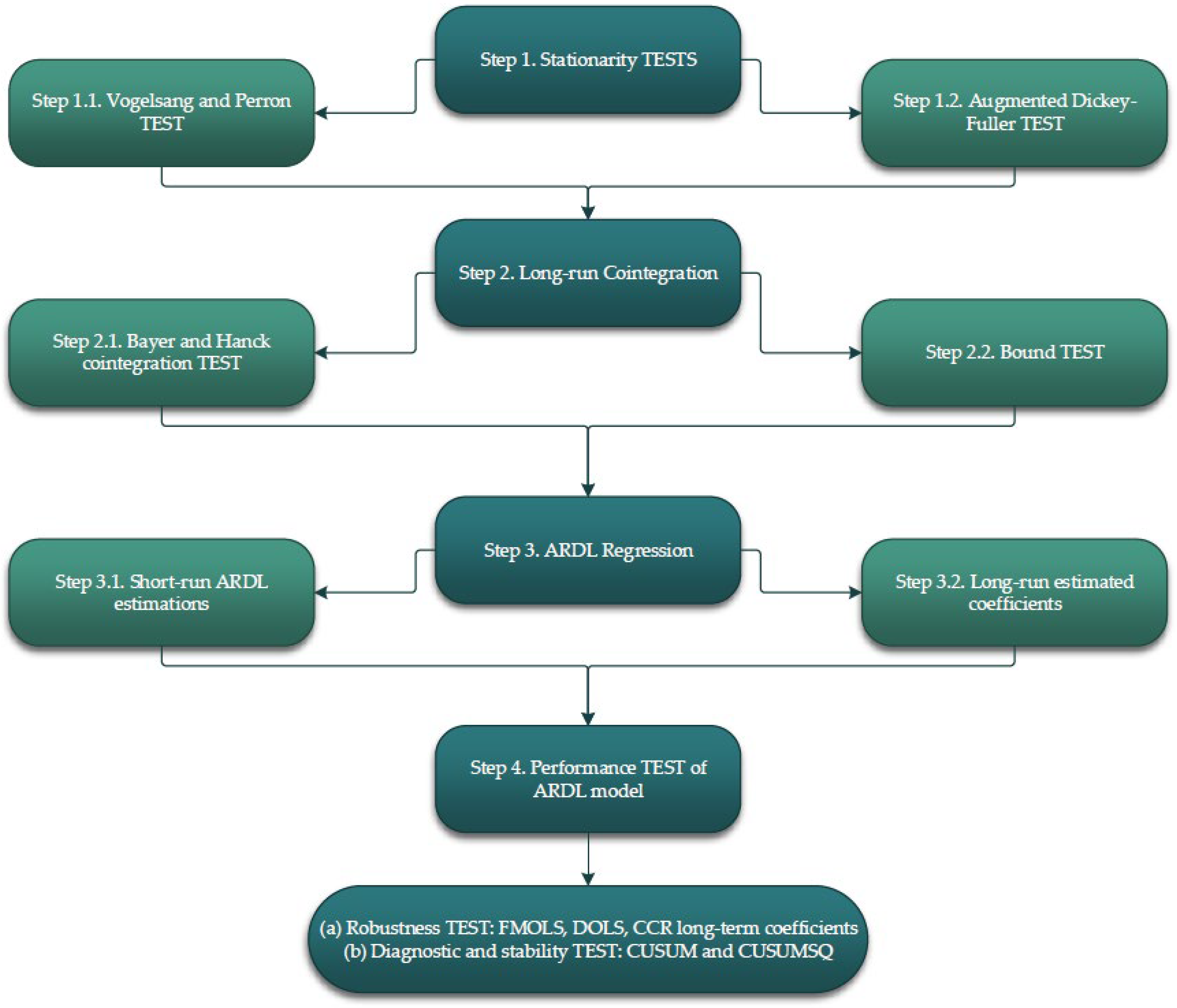
3.1. ARDL Methodology

Given the main objective described in the introduction section, this section will present the empirical findings, complex analyses, and meaningful insights derived from the applied methodology, shedding light on the critical role of economic factors in shaping the environmental landscape of Finland over the examined temporal span. To provide a clear and consistent understanding of the methodological stage of developing and validating the ARDL model, we outline the methodological steps in Figure 2.
The first step we undertook was the application of Vogeslang and Perron and ADF tests to check data stationarity. The Vogeslang and Perron test is used to verify if data series are stationary before proceeding with further analysis [37]. It helps identify any structural changes in the data under analysis. Applying the ADF test focuses on determining the stationarity of data series and identifying whether differencing is required to achieve stationary data. It is an essential step in data preparation. The second step is to verify the existence of long-term cointegration. For this stage, we used the Bayer and Hank cointegration test. This test is used to determine if there is a long-term cointegration relationship among the analyzed variables. This relationship suggests that the variables move together in the long term, having a common effect. Additionally, in this stage, we also applied the bounds test as a revalidation of the existence of long-term cointegration. If this step confirmed cointegration, we proceeded to the next stage. In step 3, short-term relationships between the analyzed variables were estimated. This helped us understand the immediate interactions between variables. Long-run estimation coefficients were also calculated, providing information about the long-term relationship between the analyzed variables. The final stage was testing the performance of the constructed ARDL model. Firstly, we applied techniques such as FMOLS, DOLS, and CCR to evaluate the model’s robustness. Subsequently, we tested the model to identify if there were issues with autocorrelation, heteroscedasticity, or deviations from a normal distribution in the model’s residuals. Additionally, we analyzed the stability of factors influencing the model’s variables.
Overall, this methodological flow aims to ensure the validity and robustness of the ARDL model, allowing researchers to draw solid conclusions and make meaningful interpretations of the relationships between the analyzed variables.
To establish a comprehensive framework for examining the relationships between FAG and its key determinants, we employed an Autoregressive Distributed Lag modeling approach. This approach offers several advantages, including the ability to capture both short-term and long-term effects and adapt to potential structural changes in the data.
The dependence equation has the form
F A G t = a 0 + a 1 G D P t + a 2 R E N P t + a 3 U R B t + ε t
Consistent with prior research, the time series were converted into their natural logarithmic forms. As a result, the estimated coefficients indicated elasticities. Implementing a logarithmic transformation on these variables helped alleviate potential fluctuations in the time-series data. The log transformation aimed to stabilize their variance [38].
Equation (1) is expressed as an ARDL (n, p, q, r) model:
F A G t = a 0 + k = 1 n a 1 Δ F A G t k + k = 1 p a 2 Δ G D P t k + k = 1 q a 3 Δ R E N P t k + k = 1 r a 4 Δ U R B t k + λ 1 F A G t 1 + λ 2 G D P t 1 + λ 3 R E N P t 1 + λ 4 U R B t 1 + ε t
In Equation (2), the first difference operator is denoted by , and ε t is the noise. We determine later the lag lengths n, p, q, and r.
A first step in applying the ARDL methodology is to check the stationarity of the data series. Stationarity is a crucial characteristic of time-series data, indicating that the mean and variance remain constant over time. To assess data stationarity, it is common practice to employ the Augmented Dickey–Fuller (ADF) test [39].
The Dickey–Fuller unit root test assesses the null hypothesis that α equals 1, where α represents the coefficient of the initial lag on y in Equation (3):
y t = c + β t + α y t 1 + Φ Δ y t 1 + e t
In Equation (3), y t 1 is the first lag of the time series, Δ y t 1 is the first difference of the time series, and e t is the error term. If the null hypothesis is accepted, then the series is non-stationary. An extension of the Dickey–Fuller unit root test [39] is the Augmented Dickey–Fuller (ADF) test, which contains a higher-order autoregressive process of order p, as shown by Equation (4):
y t = c + β t + α y t 1 + Φ 1 Δ y t 1 + Φ 2 Δ y t 2 + + Φ p Δ y t p + e t
The lag order p is determined when applying the test. The null hypothesis of the ADF test is the same as for the Dickey–Fuller test, but applied to Equation (4).
The existence of the cointegration relationship between FAG, GDP, RENP, and URB was determined using the joint cointegration test introduced in [40]. This test provides consistent outcomes by integrating four cointegration methods [41,42,43,44]. These cointegration approaches are denoted EG, JOH, BO, and BDM. This test is based on the Fisher F-statistics to furnish evidence of cointegration. In accordance with Fisher formula, the test expressions (Equations (5) and (6)) are
E G J O H = 2 [ ln P E G + ln P J O H ]
E G J O H B O B D M = 2 [ ln P E G + ln P B O + ln P B D M ]
PEG, PJOH, PBO, and PBDM represent the probabilities of the tests EG, JOH, BO, and BDM, respectively. To determine the existence of long-term relationships among the variables, the Fisher statistic was computed. The null hypothesis of no cointegration can be rejected if the Fisher statistic calculated is greater than the critical value specified by [40].
Furthermore, the results of this examination were corroborated through the utilization of the ARDL cointegration bounds test proposed by Pesaran et al. [45]. When compared to other cointegration methods, such as [41] and [42], the ARDL model has some econometric advantages. Notably, it does not need the singular integration I(1) as required by Johansen and Juselius [46]. Furthermore, it facilitates the concurrent estimation of both long-term and short-term relationships. The null hypothesis of the ARDL cointegration bounds test posits no cointegration, in contrast to the alternative hypothesis. This assessment is performed using F-statistics and involves a comparison with the critical values established by [45]. If the F-statistic surpasses the upper threshold denoted by I(1), the null hypothesis is rejected, signifying the validity of cointegration. If the F-statistic values fall below the lower threshold denoted by I(0), the null hypothesis of no cointegration is accepted. If the F-statistic values lie in the range of I(0) and I(1), the cointegration remains inconclusive.
If cointegration is present, the ECM exhibits the following structure (Equation (7)):
Δ F A G T = a 0 + k = 1 n a 1 Δ F A G t k + k = 1 p a 2 Δ G D P t k + k = 1 q a 3 Δ R E N P t k + k 1 r a 4 Δ U R B t k + Γ E C M t 1 + ε t
where Γ characterizes the short-term dynamics within the ECM. The error correction term (ECT) is expected to be statistically significant and negative, greater than −2 [47]. The negative sign signifies the speed of adjustment to the equilibrium.
The ECM Equation (7) in the ARDL model was used to analyze the dynamics of adjustment following a deviation from the long-term equilibrium relationship between the variables.
The long-term coefficients of the ARDL model were validated by supplementary testing models, like the Fully Modified Ordinary Least Squares (FMOLS) [48], Dynamic Ordinary Least Squares (DOLS) [49], and Canonical Cointegration Regression (CCR) models [50].
The robustness of the model was tested by various diagnostic tests. The normality test, Breusch–Pagan–Godfrey test, ARCH test, LM test, and Ramsey RESET test were aimed at confirming the normal distribution of the model, the absence of autocorrelation, and the stability of the results.
The model’s stability was assessed using the CUSUM and CUSUMSQ tests [51]. Research by Pesaran [52], as well as Pesaran et al. [45], contends that these two tests provide insight into the suitability of the ARDL-ECM model. Both tests involve plotting the residuals of the ECM. When the CUSUM and CUSUMSQ plots fall within the 5% critical boundary, it is not possible to reject the null hypothesis, indicating that the model’s parameters are stable.

3.2. Data Sources

In the pursuit of sustainable environmental practices and effective natural resource management, the complex relationship between economic development and forest area dynamics has become a focal point of scholarly investigation. This section delves into the crucial aspects of the data and methodology employed to scrutinize the nuanced interplay between economic indicators and forest area growth in Finland during the extensive period from 1990 to 2022.
Table 1 serves as a comprehensive repository, furnishing a concise overview of the variables under consideration and their respective sources, meticulously compiled for the specified timeframe. To gain a deeper understanding of forest area dynamics in Finland, we utilized a set of key variables, each bearing distinct significance in the context of forest conservation assessment. At the forefront of this inquiry was the dependent variable, denoted as forest area growth (FAG). This variable encapsulates the annual changes in the extent of forested regions, drawing from the forest area coverage data of the present year and its antecedent. Data for this variable were sourced from the World Bank and were employed to assess annual changes in forest expansion in Finland. RENEB signifies the percentage of electricity production derived from renewable sources, excluding hydroelectric power. Data for this variable were also provided by the World Bank and were used to evaluate the impact of renewable energy sources on forest area. GDP represents Finland’s gross domestic product, expressed in constant 2015 US dollars. This variable reflects the country’s economic performance and was included to investigate the relationship between economic development and forest area. URB indicates the percentage of urbanization within Finland’s territory. Data for urbanization were collected from the World Bank and were utilized to assess the influence of urbanization growth on forest area.
By employing these variables, we conducted an in-depth analysis of the complex relationships between economic development, urbanization, renewable energy production, and forest conservation in Finland.
To ensure consistency in understanding the abbreviated concepts used in our study, the Abbreviations section presents a description of the key abbreviated elements.

4. Results

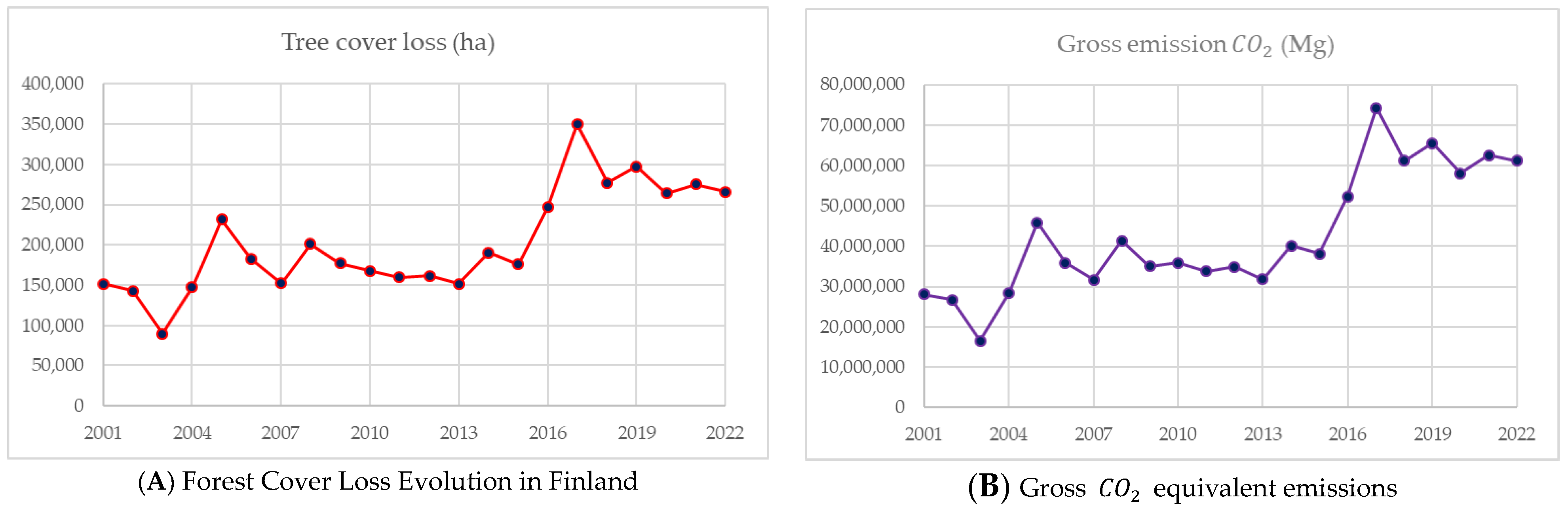
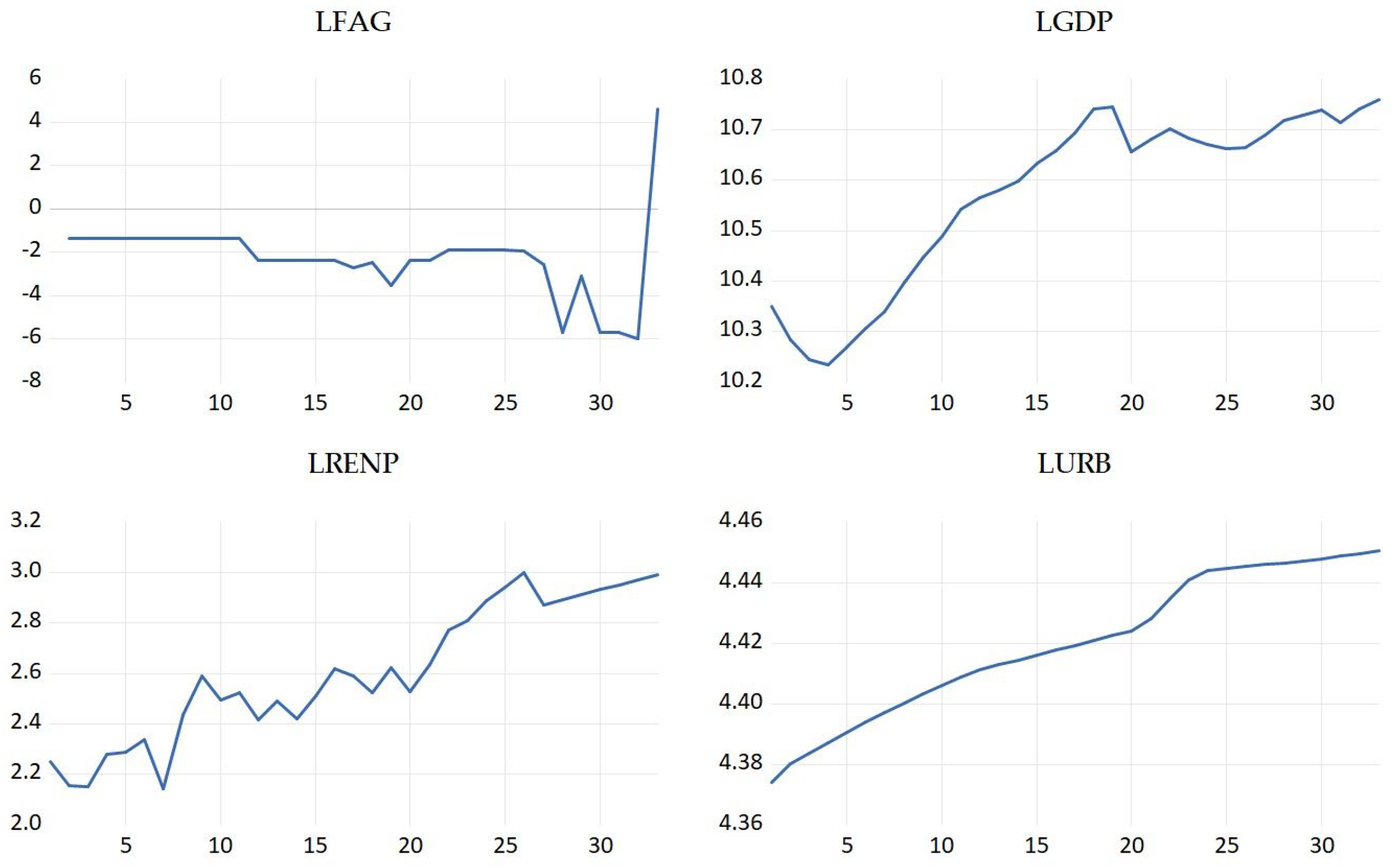
4.1. The Overall Trend of FAG and Other Factors in Finland

To begin our insightful exploration of the empirical results and the ensuing discussions, Figure 3 stands as a visual testament to the annual evolution of four pivotal indicators within the context of Finland from 1990 to 2022. The variables on the x-axis represent the years or time periods, while the values on the y-axis represent the values associated with the respective variables (FAG, GDP, RENP, URB), which are recorded in logarithmic form. Thus, on the x-axis, one has the years from 1990 to 2022, and on the y-axis, one has the corresponding logarithmic values of the mentioned variables for those years. This type of graph shows the trends and relationships between these variables over the specified period. This chronological canvas portrays the dynamic trajectories of gross domestic product (GDP), renewable energy production (RENP), urbanization (URB), and the focal variable—forest area growth (FAG).
A discerning gaze upon the depicted trends reveals an upward trajectory in GDP, RENP, and URB, signifying the robust growth in economic and urban development over the examined period. Intriguingly, FAG, the key indicator of forest area growth, exhibited a conspicuous surge in recent years, ushering in a period of heightened significance and complexity.
Drawing parallels with contemporary environmental discourse, the findings echo the observations made by Ceccherini et al. [53] on a broader European scale. Their comprehensive analysis delved into the complex dynamics of forested landscapes within the European Union (EU), spotlighting a notable surge in both forest area and biomass harvested. The stark revelation indicated a pronounced increase (+49%) in the clear cutting of forested areas across Europe during the period from 2016 to 2018, juxtaposed against the preceding years from 2011 to 2015. This surge in biomass extraction, as depicted on the biomass map, unveiled a substantial 69% upswing during the same temporal frame. Critically, these trends were primarily attributed to an escalated intensity of forest management practices, with the explicit exclusion of salvage logging post forest fires and windstorms. Notably, the lion’s share of this surge in harvested forest area was concentrated in Sweden (29%) and Finland (22%). As we traverse through the nuanced empirical landscape, the ensuing discussions will delve into the causal relationships underpinning these trends, unraveling the complex interplay between economic development, renewable energy production, urbanization, and the consequential impact on forest area growth in the Finnish context.
Table 2 contains the descriptive statistics for the logarithmized variables. The mean value of URB was 4.41, while the maximum value was 4.45. The average value for GDP was 10.57, with a low variability of 0.17. URB also showed a low variability. FAG had a platykurtic distribution, while GDP, RENP, and URB had leptokurtic distributions. All the variables were negatively skewed, except FAG.

4.2. Stationarity Analysis and Lag Selection for the VAR Model

First, basic tests were performed to assess the stationary nature of the data at both level and first difference, namely the Augmented Dickey–Fuller (ADF) test [39], shown in Table 3, and the Vogelsang and Perron breakpoint unit root test [54], shown in Table 4. A breakpoint unit root test was applied due to the fact that ADF tests can yield biased results in the presence of a structural break, as highlighted by Dogan and Ozturk [55].
It is required that all variables exhibit stationarity either at level (I(0)) or at the first difference (I(1)) to apply the ARDL bounds test. In Table 3 and Table 4, probabilities are shown in parentheses. The break years are also reported in Table 4. From Table 3 and Table 4, one can see that FAG was of integration order 0 (I(0)), while GDP, RENP, and URB were of integration order 1 (I(1)).
Hence, the ARDL technique stands as the most suitable model, being unbiased and outperforming other models designed for small sample sizes. To address endogeneity issues and eliminate residual correlation, as suggested by Ali et al. [56], it is essential to identify the suitable lag selection. All the criteria in Table 5 point to a lag number of three being the optimal choice for the Vector Autoregression (VAR) model. The columns in Table 5 are described as follows: the “Lag” column represents the number of lags used in the VAR model, the “LogL” column contains the logarithm of the maximum likelihood, the “LR” column represents the likelihood ratio associated with the proportional probability test, and the “FPE” column represents the final prediction error criterion and indicates the final prediction error. Also, the “AIC” column represents the Akaike Information Criterion, which indicates that lower values produce a better model. Additionally, the “SC” column represents the Schwartz criterion, and the “HQ” column represents the Hannan–Quinn criterion. The values marked with * in Table 5 are considered the most significant values for selecting the VAR lag order based on the criteria used.

4.3. Analysis of Cointegration and Long-Term Effects for the ARDL Model

Following this, the ARDL model was employed to assess the relationship between FAG and GDP, and RENP and URB. The initial procedure, before estimating an ARDL model, entails conducting cointegration checks through a bounds test. This test aims to either accept or reject the null hypothesis that posits the absence of cointegration. According to the AIC lag criterion, the chosen model was ARDL (1, 3, 1, 1). Therefore, n = 1, p = 3, q = 1, and r = 1. The outcomes of the ARDL cointegration bounds test are showcased in Table 6. In Table 6, the F-statistics is 6.29, exceeding the critical upper bound denoted by I(1); this indicates the presence of cointegration among the variables.
In Table 7, one can see that for both methods, the computed F-statistics values were greater than the critical values at a 5% significance level. Hence, the outcomes provided grounds for rejecting the null hypothesis (absence of cointegration) at a 5% significance level. Thus, the variables were cointegrated.
Table 8 displays the estimated long-run coefficients. From Table 8, one can see that GDP had a negative and statistically significant influence on FAG. A 1% increase in GDP caused a 4.94% decrease in FAG.
This negative relationship between GDP per capita and the annual growth of forested areas can be explained by several factors specific to the Finnish context. Finland has evolved into a highly developed and industrialized nation with a substantial GDP per capita. As the country attained advanced economic levels, it underwent a transition from a forestry-centric economy to one that is predominantly industrial and service-oriented. This transition may have resulted in a decrease in the annual growth of forested areas as land is needed for urbanization, infrastructure, and industrial activities. Finland boasts a longstanding tradition of implementing sustainable forest management practices. The Finnish forest industry operates under robust regulations, ensuring that the pace of deforestation is carefully controlled to promote the sustained growth of forested areas over the long term. This approach aims to strike a balance between economic development and ecological preservation.
A 1% increase in RENP led to a 1.70% increase in FAG. When renewable energy production relies on sustainably sourced biomass, it can encourage the growth of forested areas. Sustainable harvesting practices ensure that the rate of tree growth exceeds the rate of tree removal for energy production, leading to a net increase in forested land. The policies and practices that Finland has adopted strike a balance between renewable energy production and forest conservation. This means that while biomass may be used for energy, steps are taken to ensure that the overall forested area increases over time. The positive correlation between the use of renewable energy and the expansion of forested areas is confirmed by [1,18,23]. When cleaner energy sources are more accessible, there is a reduced reliance on forest products for fuel.
A 1% increase in URB led to an 8.68% increase in FAG. This positive relationship aligns with Finland’s strong tradition of urban planning and development. Many Finish cities prioritize parks, green spaces, and forests within their urban landscapes. Forests and green areas are integrated into urban environments, promoting their growth and preservation. Urbanization in Finland is often accompanied by policies and initiatives that aim to protect biodiversity. As urbanization continues, the importance of these green areas for carbon sequestration and offsetting emissions is recognized. The positive impact of URB on FAG is contingent on effective urban planning and policies that prioritize green spaces and sustainable practices.
In Finland, urbanization is viewed not merely as a driver of built environment expansion but as an opportunity to enrich the coexistence of urban areas and nature. This approach aims to cultivate the growth and preservation of forested areas amidst urban development.
The ARDL-ECM model results are summarized in Table 9. The ECT registered a value of −1.46, which is negative and statistically significant at the 5% level, indicating the presence of cointegration. The adjustment speed toward the long-term equilibrium following short-term deviations stood at 146%. This adjustment coefficient of −1.46 signifies that the deviations in FAG from equilibrium were corrected by 146% in the subsequent period. In this case, the ECT fell within the range of −2 to −1, causing dampened oscillations.
The explanatory variables accounted for 69% of the total variation in FAG, as explained by the Adjusted R-squared value.
The short-term dynamics of FAG, GDP, URN, and RENP are captured in Table 9. In the short term, the positive impact of GDP on FAG can be explained by the resources available for conservation efforts. The Finish government and organizations invest in reforestation and afforestation programs. Also, short-term fluctuations in demand for forest products, like timber or paper, can result in forestry operations being scaled back, allowing forests to regenerate. In the short term, URB and RENP had a positive impact on FAG, as in the long term.

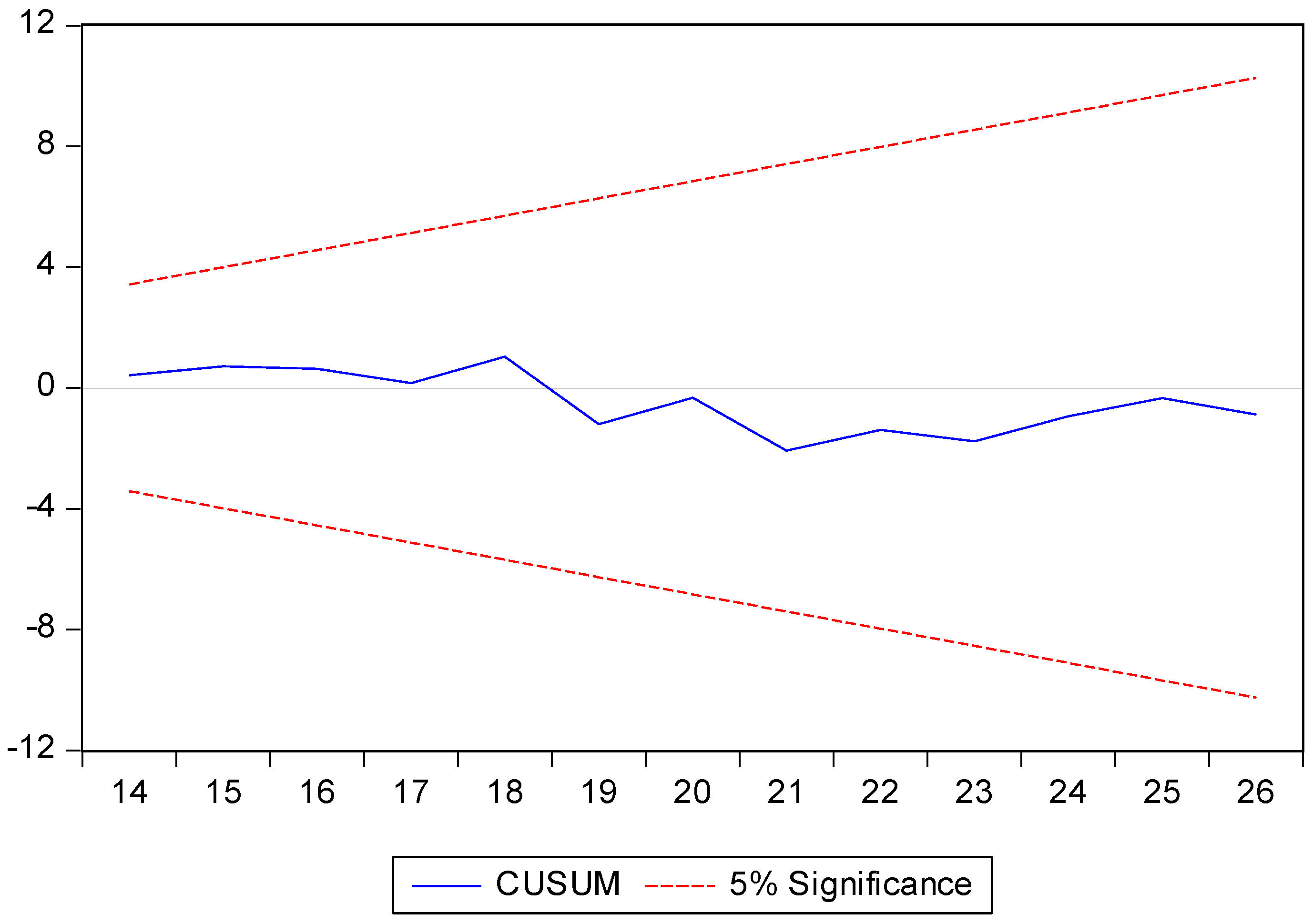
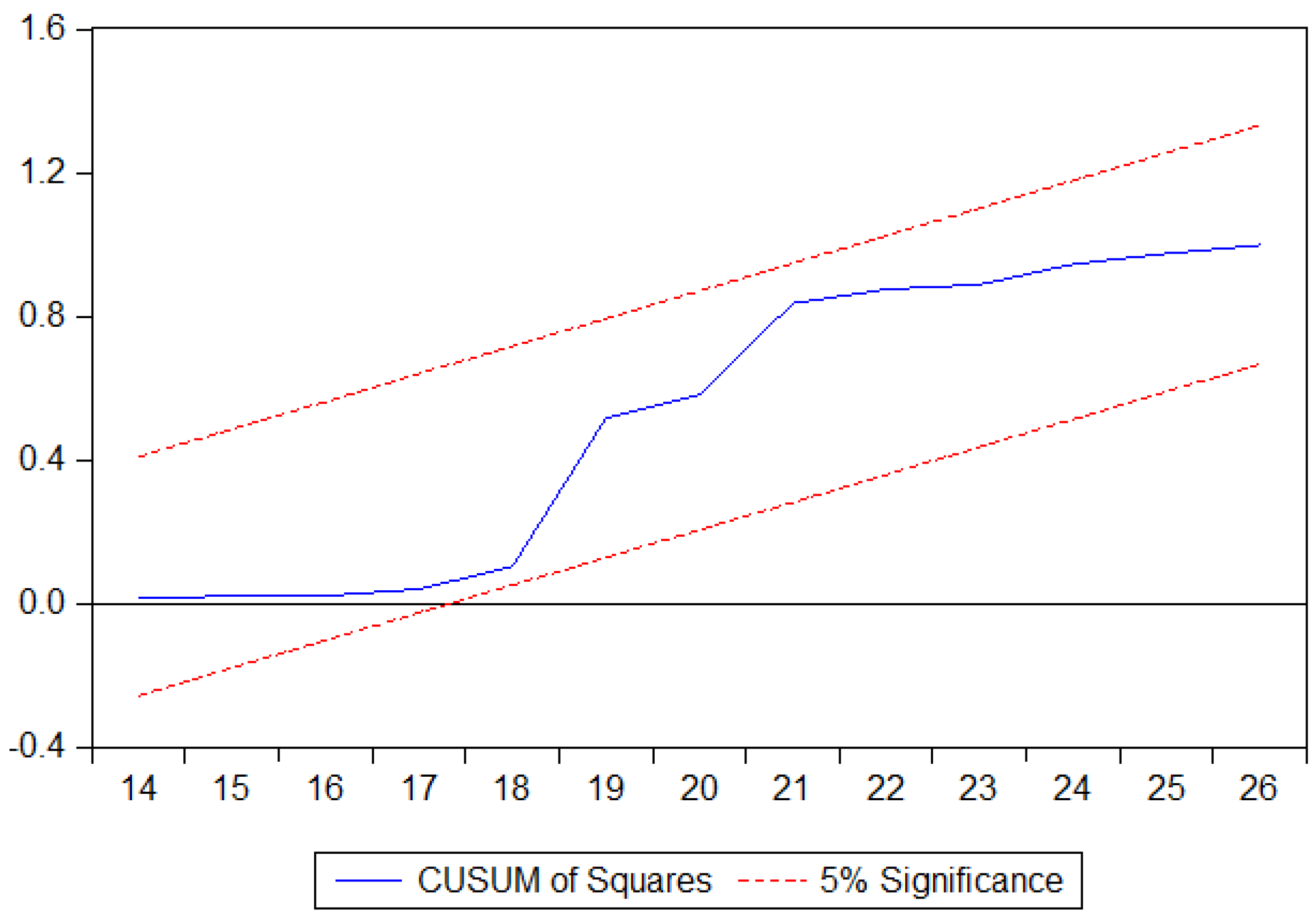
4.4. Evaluation of Model Assumptions and Diagnostic Analysis

In addition, this study employed the FMOLS (Fully Modified Ordinary Least Squares), DOLS (Dynamic Ordinary Least Squares), and CCR (Canonical Cointegration Regression) techniques to validate the findings established in the ARDL model. These three techniques were essential to ensure that the statistical analysis was accurate for the research variables, with respect to the previously established cointegration relationships. One can notice from Table 10 that most signs of the FMOLS, DOLS, and CCR tests are consistent with the ARDL long-run results.
Table 11 displays four null hypotheses ( H 0 ) for the diagnostic tests along with their corresponding values. It is noteworthy that the p-values for the tests of serial correlation, heteroscedasticity, and Jarque–Bera normality all exceeded 0.05, which is a positive outcome. As a result, this model did not exhibit autocorrelation or heteroscedasticity. Additionally, given that the probability of the Jarque–Bera test surpassed 0.05 and the Jarque–Bera value fell below 5, it can be concluded that the residuals followed a normal distribution. The Ramsey RESET test indicated that the model was appropriately specified, thereby suggesting the absence of instability in the factors determining FAG.
We evaluated the model’s stability through the CUSUM and CUSUMSQ tests, plotted in Figure 4 and Figure 5. Within these graphs, the blue line represents the CUSUM values (Figure 4) and the CUSUMSQ values (Figure 5) calculated for each data point in the time series. The CUSUM is the cumulative sum of the differences between the observed values and the expected values (estimated values or mean values) for each data point. The CUSUMSQ represents the cumulative sum of the squares of these differences. The blue line can provide insights into the moments when structural changes occurred in the analyzed data. If the blue line exceeds the defined boundaries (represented by the red lines) at a significance level of 5%, it may suggest the presence of a significant change in the data at that particular moment. Both tests indicated that the model’s parameters were stable, as both plots fell within the 5% critical threshold marked by the red dashed line. This underscores the model’s appropriateness for making forecasts.
The examination of the ARDL-ECM model validated the presence of dynamic properties in the time series. Consequently, given the robustness of the model, it exhibited a strong fit, thereby enabling the formulation of policy recommendations.

5. Conclusions and Recommendations

This research analyzed the nexus between forest area growth, electricity production from renewable sources, GDP, and urbanization for Finland during the period 1990–2022. The unit root test results indicated that the variables exhibited integration of order zero (I(0)) and order one (I(1)). Additionally, the cointegration test implied the existence of a long-term relationship among these variables. The error correction term indicated that the speed of forest area growth adjustment to equilibrium was high, at about 146%.
In the long-term analysis, forest area growth was negatively connected with economic growth (research question 1, RQ1) and positively connected with electricity production from renewable sources and urbanization (research question 2, RQ2). In the short term, forest area growth was positively connected with all regressors (RQ1/RQ2).
According to the empirical findings, the following policy recommendations are suggested. The surge in economic activity should ideally occur in contexts where environmental sustainability and forest conservation are prioritized. The combination of population growth and urbanization must be accompanied by sustainable land-use practices to avert an increase in deforestation. Urban growth could be guided by ecological practices, including efficient land use and maintaining green areas within cities. The implementation of sustainable forest management policies could involve measures such as sustainable harvesting, natural forest regeneration, and biodiversity protection. The specific aspects of Finnish forest conservation are interconnected with global trends or affected by external factors. Policymakers may consider strengthening international collaborations to address transboundary issues. In summary, the ARDL-based evaluation of forest conservation in Finland can have far-reaching policy implications, influencing strategies, resource allocation, international collaboration, community engagement, climate change adaptation, monitoring frameworks, economic considerations, and policy stability. Additionally, promoting education and public awareness about the importance of forests and the necessity of sustainable development can contribute to supporting these policies. Well-informed citizens are more likely to endorse initiatives aimed at conserving natural resources. Policymakers should carefully consider these implications to ensure the sustainability and success of forest conservation efforts.
Furthermore, regarding the use of the results of our study in other countries with different economic characteristics and conservation policies, our study can provide an analytical and methodological model that is applicable in various similar or different contexts. For example, countries facing similar issues related to deforestation and economic development can adapt this methodology to assess the specific impact of their local factors on forest resources. Additionally, the study can serve as a source of inspiration for the development of forest conservation policies and strategies in a variety of national and regional contexts. However, it is important to consider the specific differences of each country and the local nuances in decision making and environmental policy implementation. Alternatively, the exchange of best practices and lessons learned from Finland could contribute to the development and implementation of more efficient and sustainable forest conservation strategies in other countries. Thus, the results and methodology of this study can contribute to global forest conservation efforts and the promotion of sustainable development.
Additionally, researchers and industry specialists aiming to utilize the findings of our work must consider that despite the positive results of clean energy utilization, there are still numerous obstacles and challenges that countries need to overcome to successfully implement these technologies [57]. Transitioning to clean energy sources often requires significant investments in infrastructure and new technologies, which can be challenging for countries with limited financial resources [58]. Moreover, many countries still heavily rely on traditional energy sources such as fossil fuels. Shifting to clean energy sources may entail significant changes in infrastructure and the economy. Additionally, the lack of adequate regulations and policies to promote clean energy can be a major hindrance to the implementation of these technologies [59,60].
Certainly, additional concerted endeavors are necessary to devise strategies for sustaining biodiversity in both managed and protected forests. Achieving genuinely sustainable forests and forestry in Finnish society will depend on these collective efforts.
Future studies should analyze additional factors that could influence emission reduction and environmental sustainability, while taking account of the implications from structural breaks in the data. These factors might encompass practices like recycling products and minimizing water and electricity consumption. Additionally, considering that our study focused on Finland in general, future research could include a more detailed spatial analysis, examining how changes in forest area vary across different regions of the country. This might involve assessing the sensitivity of specific areas and the qualitative implications of changes in these areas. Expanding the research to include comparisons with other countries could provide a broader perspective on the effectiveness of forest conservation policies and the involved economic and social factors. Moreover, the continued monitoring and analysis of long-term trends concerning forest area growth, in the context of the constant evolution of economic and social factors, and a detailed analysis of how various public policies (both national and international) influence forest conservation and sustainable development could be another direction for research.

Author Contributions

Conceptualization, I.G., J.K., and I.N.; methodology, I.G. and J.K.; software, I.G. and I.N.; validation, I.G., J.K., and I.N.; formal analysis, I.G.; investigation, I.G., J.K., and I.N.; resources, I.G., J.K., and I.N.; data curation, I.N.; writing—original draft preparation, I.G. and J.K.; writing—review and editing, I.G. and I.N.; visualization, I.G., J.K., and I.N.; supervision, I.G. and I.N.; project administration, I.G., J.K., and I.N. All authors have read and agreed to the published version of the manuscript.

Funding

This research received no external funding.

Institutional Review Board Statement

Not applicable.

Informed Consent Statement

Not applicable.

Data Availability Statement

Data are available upon request.

Conflicts of Interest

The authors declare no conflicts of interest.

Abbreviations

ARDLAutoregressive Distributed Lag
ECMError correction model
GDPGross domestic product
GHGGreenhouse gas
RENPRenewable energy production
URBUrbanization
FAForest area
FAGForest area growth
FMOLSFully Modified Ordinary Least Squares
DOLSDynamic Ordinary Least Squares
CCRCanonical Cointegration Regression
CUSUMCumulative sum
CUSUMSQCumulative sum of squares

References

  1. Tanner, A.M.; Johnston, A.L. The Impact of Rural Electric Access on Deforestation Rates. World Dev. 2017, 94, 174–185. [Google Scholar] [CrossRef]
  2. Prochazka, P.; Abrham, J.; Cerveny, J.; Kobera, L.; Sanova, P.; Benes, D.; Fink, J.-M.; Jiraskova, E.; Primasova, S.; Soukupova, J.; et al. Understanding the Socio-Economic Causes of Deforestation: A Global Perspective. Front. For. Glob. Change 2023, 6, 1288365. [Google Scholar] [CrossRef]
  3. Belušić, D.; Fuentes-Franco, R.; Strandberg, G.; Jukimenko, A. Afforestation Reduces Cyclone Intensity and Precipitation Extremes over Europe. Environ. Res. Lett. 2019, 14, 074009. [Google Scholar] [CrossRef]
  4. Rădulescu, C.V.; Bran, F.; Ciuvăț, A.L.; Bodislav, D.A.; Buzoianu, O.C.; Ștefănescu, M.; Burlacu, S. Decoupling the Economic Development from Resource Consumption: Implications and Challenges in Assessing the Evolution of Forest Area in Romania. Land 2022, 11, 1097. [Google Scholar] [CrossRef]
  5. Majava, A.; Vadén, T.; Toivanen, T.; Järvensivu, P.; Lähde, V.; Eronen, J.T. Sectoral Low-Carbon Roadmaps and the Role of Forest Biomass in Finland’s Carbon Neutrality 2035 Target. Energy Strategy Rev. 2022, 41, 100836. [Google Scholar] [CrossRef]
  6. Triviño, M.; Potterf, M.; Tijerín, J.; Ruiz-Benito, P.; Burgas, D.; Eyvindson, K.; Blattert, C.; Mönkkönen, M.; Duflot, R. Enhancing Resilience of Boreal Forests Through Management Under Global Change: A Review. Curr. Landsc. Ecol. Rep. 2023, 8, 103–118. [Google Scholar] [CrossRef]
  7. Finnish Forests. Finland Is a Country That Lives off Its Forests—Culturally, Socially, and Economically. Available online: https://toolbox.finland.fi/wp-content/uploads/sites/2/2023/06/suomi-finland-narrative-packages-finnish-forests.pdf (accessed on 12 October 2023).
  8. European Parliament Sustainable Forestry in Finland. Available online: https://www.europarl.europa.eu/RegData/etudes/STUD/2016/578979/IPOL_STU(2016)578979_EN.pdf (accessed on 12 October 2023).
  9. Global Forest Watch. Available online: https://www.globalforestwatch.org/dashboards/global/ (accessed on 12 October 2023).
  10. França, L.C.D.J.; Júnior, F.W.A.; Jarochinski E Silva, C.S.; Monti, C.A.U.; Ferreira, T.C.; Santana, C.J.D.O.; Gomide, L.R. Forest Landscape Planning and Management: A State-of-the-Art Review. Trees For. People 2022, 8, 100275. [Google Scholar] [CrossRef]
  11. Yamamoto, Y.; Matsumoto, K. The Effect of Forest Certification on Conservation and Sustainable Forest Management. J. Clean. Prod. 2022, 363, 132374. [Google Scholar] [CrossRef]
  12. Mönkkönen, M.; Aakala, T.; Burgas, D.; Duflot, R.; Eyvindson, K.; Kouki, J.; Laaksonen, T.; Punttila, P. More Wood but Less Biodiversity in Forests in Finland: A Historical Evaluation. Memo. Soc. Fauna Flora Fenn. 2022, 98, 1–11. [Google Scholar]
  13. Aakala, T.; Kulha, N.; Kuuluvainen, T. Human Impact on Forests in Early Twentieth Century Finland. Landsc. Ecol. 2023, 38, 2417–2431. [Google Scholar] [CrossRef]
  14. Murshed, M.; Ferdaus, J.; Rashid, S.; Tanha, M.M.; Islam, M.J. The Environmental Kuznets Curve Hypothesis for Deforestation in Bangladesh: An ARDL Analysis with Multiple Structural Breaks. Energ. Ecol. Environ. 2021, 6, 111–132. [Google Scholar] [CrossRef]
  15. Georgescu, I.; Kinnunen, J. The Role of Foreign Direct Investments, Urbanization, Productivity, and Energy Consumption in Finland’s Carbon Emissions: An ARDL Approach. Environ. Sci. Pollut. Res. 2023, 30, 87685–87694. [Google Scholar] [CrossRef]
  16. Cozma, A.-C.; Coroș, M.M.; Pop, A.M.; Gavrilescu, I.; Dinucă, N.C. Corruption, Deforestation, and Tourism—Europe Case Study. Heliyon 2023, 9, e19075. [Google Scholar] [CrossRef] [PubMed]
  17. Ditta, A.; Asim, H.; Rehman, H.U. An Econometric Analysis of Exigent Determinants of Trade Balance in Finland: An Autoregressive Distributed Lag (ARDL) Approach. Rev. Appl. Manag. Soc. Sci. 2020, 3, 347–360. [Google Scholar] [CrossRef]
  18. Ponce, P.; Del Río-Rama, M.D.L.C.; Álvarez-García, J.; Oliveira, C. Forest Conservation and Renewable Energy Consumption: An ARDL Approach. Forests 2021, 12, 255. [Google Scholar] [CrossRef]
  19. Ahmed, K.; Shahbaz, M.; Qasim, A.; Long, W. The Linkages between Deforestation, Energy and Growth for Environmental Degradation in Pakistan. Ecol. Indic. 2015, 49, 95–103. [Google Scholar] [CrossRef]
  20. Bhattacharyya, S.C.; Ohiare, S. The Chinese Electricity Access Model for Rural Electrification: Approach, Experience and Lessons for Others. Energy Policy 2012, 49, 676–687. [Google Scholar] [CrossRef]
  21. Bakehe, N.P. L’accès à l’électricité: Une Solution Pour Réduire La Déforestation En Afrique? Afr. Dev. Rev. 2020, 32, 338–348. [Google Scholar] [CrossRef]
  22. Woldemedhin, D.G.; Assefa, E.; Seyoum, A. Forest Covers, Energy Use, and Economic Growth Nexus in the Tropics: A Case of Ethiopia. Trees For. People 2022, 8, 100266. [Google Scholar] [CrossRef]
  23. Nazir, M.S.; Bilal, M.; Sohail, H.M.; Liu, B.; Chen, W.; Iqbal, H.M.N. Impacts of Renewable Energy Atlas: Reaping the Benefits of Renewables and Biodiversity Threats. Int. J. Hydrog. Energy 2020, 45, 22113–22124. [Google Scholar] [CrossRef]
  24. Bakehe, N.P.; Hassan, R. The Effects of Access to Clean Fuels and Technologies for Cooking on Deforestation in Developing Countries. J. Knowl. Econ. 2023, 14, 2561–2577. [Google Scholar] [CrossRef]
  25. Acheampong, A.O.; Opoku, E.E.O. Energy Justice, Democracy and Deforestation. J. Environ. Manag. 2023, 341, 118012. [Google Scholar] [CrossRef]
  26. Omar Makame, M. Adoption of Improved Stoves and Deforestation in Zanzibar. Manag. Environ. Qual. Int. J. 2007, 18, 353–365. [Google Scholar] [CrossRef]
  27. Ajanaku, B.A.; Collins, A.R. Economic Growth and Deforestation in African Countries: Is the Environmental Kuznets Curve Hypothesis Applicable? For. Policy Econ. 2021, 129, 102488. [Google Scholar] [CrossRef]
  28. Caravaggio, N. A Global Empirical Re-Assessment of the Environmental Kuznets Curve for Deforestation. For. Policy Econ. 2020, 119, 102282. [Google Scholar] [CrossRef]
  29. Zambrano-Monserrate, M.A.; Carvajal-Lara, C.; Urgilés-Sanchez, R.; Ruano, M.A. Deforestation as an Indicator of Environmental Degradation: Analysis of Five European Countries. Ecol. Indic. 2018, 90, 1–8. [Google Scholar] [CrossRef]
  30. Tsiantikoudis, S.; Zafeiriou, E.; Kyriakopoulos, G.; Arabatzis, G. Revising the Environmental Kuznets Curve for Deforestation: An Empirical Study for Bulgaria. Sustainability 2019, 11, 4364. [Google Scholar] [CrossRef]
  31. Arcand, J.-L.; Guillaumont, P.; Jeanneney, S.G. Deforestation and the Real Exchange Rate. J. Dev. Econ. 2008, 86, 242–262. [Google Scholar] [CrossRef]
  32. Faria, W.R.; Almeida, A.N. Relationship between Openness to Trade and Deforestation: Empirical Evidence from the Brazilian Amazon. Ecol. Econ. 2016, 121, 85–97. [Google Scholar] [CrossRef]
  33. Nathaniel, S.P.; Bekun, F.V. Environmental Management amidst Energy Use, Urbanization, Trade Openness, and Deforestation: The Nigerian Experience. J. Public Aff. 2020, 20, e2037. [Google Scholar] [CrossRef]
  34. Yameogo, C.E.W. Globalization, Urbanization, and Deforestation Linkage in Burkina Faso. Environ. Sci. Pollut. Res. 2021, 28, 22011–22021. [Google Scholar] [CrossRef] [PubMed]
  35. Rydning Gaarder, A.; Vadlamannati, K.C. Does Democracy Guarantee (de)Forestation? An Empirical Analysis. Int. Area Stud. Rev. 2017, 20, 97–121. [Google Scholar] [CrossRef]
  36. Moreira-Dantas, I.R.; Söder, M. Global Deforestation Revisited: The Role of Weak Institutions. Land Use Policy 2022, 122, 106383. [Google Scholar] [CrossRef]
  37. Russo, E.; Foster-McGregor, N. Characterizing Growth Instability: New Evidence on Unit Roots and Structural Breaks in Countries’ Long Run Trajectories. J. Evol. Econ. 2022, 32, 713–756. [Google Scholar] [CrossRef]
  38. Lütkepohl, H.; Xu, F. The Role of the Log Transformation in Forecasting Economic Variables. Empir. Econ. 2012, 42, 619–638. [Google Scholar] [CrossRef]
  39. Dickey, D.A.; Fuller, W.A. Distribution of the Estimators for Autoregressive Time Series with a Unit Root. J. Am. Stat. Assoc. 1979, 74, 427. [Google Scholar] [CrossRef]
  40. Bayer, C.; Hanck, C. Combining Non-cointegration Tests. J. Time Ser. Anal. 2013, 34, 83–95. [Google Scholar] [CrossRef]
  41. Engle, R.F.; Granger, C.W.J. Co-Integration and Error Correction: Representation, Estimation, and Testing. Econometrica 1987, 55, 251. [Google Scholar] [CrossRef]
  42. Johansen, S. Statistical Analysis of Cointegration Vectors. J. Econ. Dyn. Control. 1988, 12, 231–254. [Google Scholar] [CrossRef]
  43. Peter Boswijk, H. Testing for an Unstable Root in Conditional and Structural Error Correction Models. J. Econom. 1994, 63, 37–60. [Google Scholar] [CrossRef]
  44. Banerjee, A.; Dolado, J.; Mestre, R. Error-correction Mechanism Tests for Cointegration in a Single-equation Framework. J. Time Ser. Anal. 1998, 19, 267–283. [Google Scholar] [CrossRef]
  45. Pesaran, M.H.; Shin, Y.; Smith, R.J. Bounds Testing Approaches to the Analysis of Level Relationships. J. Appl. Econom. 2001, 16, 289–326. [Google Scholar] [CrossRef]
  46. Johansen, S.; Juselius, K. Maximum Likelihood Estimation and Inference on Cointegration—With Applications to the Demand for Money. Oxf. Bull. Econ. Stat. 1990, 52, 169–210. [Google Scholar] [CrossRef]
  47. Samargandi, N.; Fidrmuc, J.; Ghosh, S. Is the Relationship Between Financial Development and Economic Growth Monotonic? Evidence from a Sample of Middle-Income Countries. World Dev. 2015, 68, 66–81. [Google Scholar] [CrossRef]
  48. Phillips, P.C.B.; Hansen, B.E. Statistical Inference in Instrumental Variables Regression with I(1) Processes. Rev. Econ. Stud. 1990, 57, 99. [Google Scholar] [CrossRef]
  49. Stock, J.H.; Watson, M.W. A Simple Estimator of Cointegrating Vectors in Higher Order Integrated Systems. Econometrica 1993, 61, 783. [Google Scholar] [CrossRef]
  50. Park, J.Y. Canonical Cointegrating Regressions. Econometrica 1992, 60, 119. [Google Scholar] [CrossRef]
  51. Brown, R.L.; Durbin, J.; Evans, J.M. Techniques for Testing the Constancy of Regression Relationships Over Time. J. R. Stat. Soc. Ser. B Methodol. 1975, 37, 149–163. [Google Scholar] [CrossRef]
  52. Pesaran, M.H. An Autoregressive Distributed-Lag Modelling Approach to Cointegration Analysis. In Econometrics and Economic Theory in the 20th Century: The Ragnar Frisch Centennial Symposium; Strøm, S., Ed.; Cambridge University Press: New York, NY, USA, 1998; pp. 371–413. ISBN 978-0-521-63323-9. [Google Scholar]
  53. Ceccherini, G.; Duveiller, G.; Grassi, G.; Lemoine, G.; Avitabile, V.; Pilli, R.; Cescatti, A. Abrupt Increase in Harvested Forest Area over Europe after 2015. Nature 2020, 583, 72–77. [Google Scholar] [CrossRef]
  54. Vogelsang, T.J.; Perron, P. Additional Tests for a Unit Root Allowing for a Break in the Trend Function at an Unknown Time. Int. Econ. Rev. 1998, 39, 1073. [Google Scholar] [CrossRef]
  55. Dogan, E.; Ozturk, I. The Influence of Renewable and Non-Renewable Energy Consumption and Real Income on CO2 Emissions in the USA: Evidence from Structural Break Tests. Environ. Sci. Pollut. Res. 2017, 24, 10846–10854. [Google Scholar] [CrossRef] [PubMed]
  56. Ali, H.S.; Law, S.H.; Zannah, T.I. Dynamic Impact of Urbanization, Economic Growth, Energy Consumption, and Trade Openness on CO2 Emissions in Nigeria. Environ. Sci. Pollut. Res. 2016, 23, 12435–12443. [Google Scholar] [CrossRef] [PubMed]
  57. Lv, Y. Transitioning to Sustainable Energy: Opportunities, Challenges, and the Potential of Blockchain Technology. Front. Energy Res. 2023, 11, 1258044. [Google Scholar] [CrossRef]
  58. Chipangamate, N.S.; Nwaila, G.T. Assessment of Challenges and Strategies for Driving Energy Transitions in Emerging Markets: A Socio-Technological Systems Perspective. Energy Geosci. 2024, 5, 100257. [Google Scholar] [CrossRef]
  59. Farghali, M.; Osman, A.I.; Chen, Z.; Abdelhaleem, A.; Ihara, I.; Mohamed, I.M.A.; Yap, P.-S.; Rooney, D.W. Social, Environmental, and Economic Consequences of Integrating Renewable Energies in the Electricity Sector: A Review. Environ. Chem. Lett. 2023, 21, 1381–1418. [Google Scholar] [CrossRef]
  60. Gielen, D.; Boshell, F.; Saygin, D.; Bazilian, M.D.; Wagner, N.; Gorini, R. The Role of Renewable Energy in the Global Energy Transformation. Energy Strategy Rev. 2019, 24, 38–50. [Google Scholar] [CrossRef]
Figure 1. Forest cover loss in Finland (A) and gross C O 2 equivalent emissions (B) according to [9].
Sustainability 16 00612 g001
Figure 2. Methodological flow of ARDL model.
Sustainability 16 00612 g002
Figure 3. The evolution of FAG, GDP, RENP, and URB (logarithmized variables) for Finland (1990–2022).
Sustainability 16 00612 g003
Figure 4. CUSUM plot at 5% level of significance.
Sustainability 16 00612 g004
Figure 5. CUSUMSQ plot at 5% level of significance.
Sustainability 16 00612 g005
Table 1. Factors and data origins.
FactorAbbreviationMeasurement UnitData Origin
Forest areaFA% of land areaWorld Bank
Electricity production from renewable sources, excluding hydroelectricRENB% of totalWorld Bank
Gross domestic productGDPConstant 2015 USDWorld Bank
UrbanizationURB%World Bank
Table 2. Summary statistics.
FAGGDPRENBURB
Mean−2.2310.572.594.41
Median−1.9210.652.554.41
Maximum4.6010.752.994.45
Minimum−5.9710.232.144.38
Std. Dev.1.920.170.260.02
Skewness0.71−0.82−0.01−0.10
Kurtosis7.342.201.951.85
Jarque–Bera26.174.171.361.68
Probability0.000.120.500.42
Table 3. ADF unit root test results.
VariableLevelFirst DifferenceOrder of Integration
t-Statisticst-Statistics
FAG−2.30 (0.02)−1.93 (0.05)I(0)
GDP2.15 (0.99)−3.49 (0.00)I(1)
RENP1.35 (0.95)−5.71 (0.00)I(1)
URB1.70 (0.97)−1.88 (0.05)I(1)
Table 4. Vogelsang and Perron breakpoint unit root test results.
Variablet-StatisticsBreak YearOrder of Integration
LevelFirst DifferenceLevelFirst Difference
FAG−4.96 (0.00)−7.02 (0.00)20002021I(0)
GDP−3.72 (0.26)−6.98 (0.00)19962008I(1)
RENP−1.99 (0.98)−6.86 (0.00)20101998I(1)
URB−8.73 (0.00)−4.87 (0.01)20092013I(1)
Table 5. VAR lag order selection criteria.
LagLogLLRFPEAICSCHQ
0104.56NA1.25 × 10 9 −5.14−8.94−9.09
1195.41140.391.44 × 10 12 −15.94−14.95−15.71
2217.1325.661.02 × 10 12 −16.46−14.68−16.04
3255.7531.60 *2.15 × 10 12 *−18.52 *−15.94 *−17.91 *
Table 6. Results of ARDL cointegration bounds test.
Test StatisticValueK (Number of Regressors)
F-statistic6.293
Critical value bounds
SignificanceI(0)I(1)
10%2.673.58
5%3.274.30
1%4.615.96
Table 7. Bayer and Hanck cointegration test results.
Fisher Statistics
EG-JOH-BO-BDM
Fisher Statistics
EG-JOH
EG-JOH-BO-BDM
Fisher Critical Value at 5% Level
EG-JOH
Fisher Critical Value at 5% Level
Inference
111.6356.3520.4810.63Cointegration
Table 8. The long-run estimated coefficients.
VariableCoefficientt-StatisticsProb.
GDP−4.94−7.810.00
URB8.680.690.49
RENP1.702.230.04
C7.170.140.84
Table 9. The short-run ARDL (1,3,1,1) estimation.
VariableCoefficientt-StatisticsProb.
D(GDP)0.600.310.754
D(GDP(−1))1.010.550.587
D(GDP(−2))3.141.910.076
D(URB)141.185.570.001
D(RENP)1.021.890.081
CointEq(−1)−1.46−6.410.000
R-squared 0.76
Adjusted R-squared 0.69
Table 10. FMOLS, DOLS, and CCR long-term coefficients.
VariableFMOLSDOLSCCR
GDP−4.80 ***
(−5.93)
−2.95 ***
(−4.29)
−4.72 ***
(−0.24)
URB6.54
(0.49)
−28.11 *
(−2.21)
3.48
(0.28)
RENP1.38 *
(1.70)
4.04 ***
(3.17)
1.58 *
(1.71)
C16.29
(0.32)
142.21 **
(2.72)
28.37
(0.58)
*, **, *** indicate the significance of variables at 10%, 5%, and 1% levels, respectively.
Table 11. Results of diagnostic and stability tests.
Test H 0 Decision
Statistics (p-Value)
Serial correlationThere is no serial correlation in the residuals Accept   H 0
1.59 (0.25)
HeteroscedasticityThere is no autoregressive conditional heteroscedasticity Accept   H 0
0.07 (0.78)
Normal distributionNormal distribution Accept   H 0
0.01 (0.99)
Ramset RESETThe absence of model misspecification Accept   H 0
3.54 (0.06)
Disclaimer/Publisher’s Note: The statements, opinions and data contained in all publications are solely those of the individual author(s) and contributor(s) and not of MDPI and/or the editor(s). MDPI and/or the editor(s) disclaim responsibility for any injury to people or property resulting from any ideas, methods, instructions or products referred to in the content.

