
Stakeholder-Driven Policies and Scenarios of Land System Change and Environmental Impacts: A Case Study of Owyhee County, Idaho, United States


Abstract
:1. Introduction
2. Materials and Methods
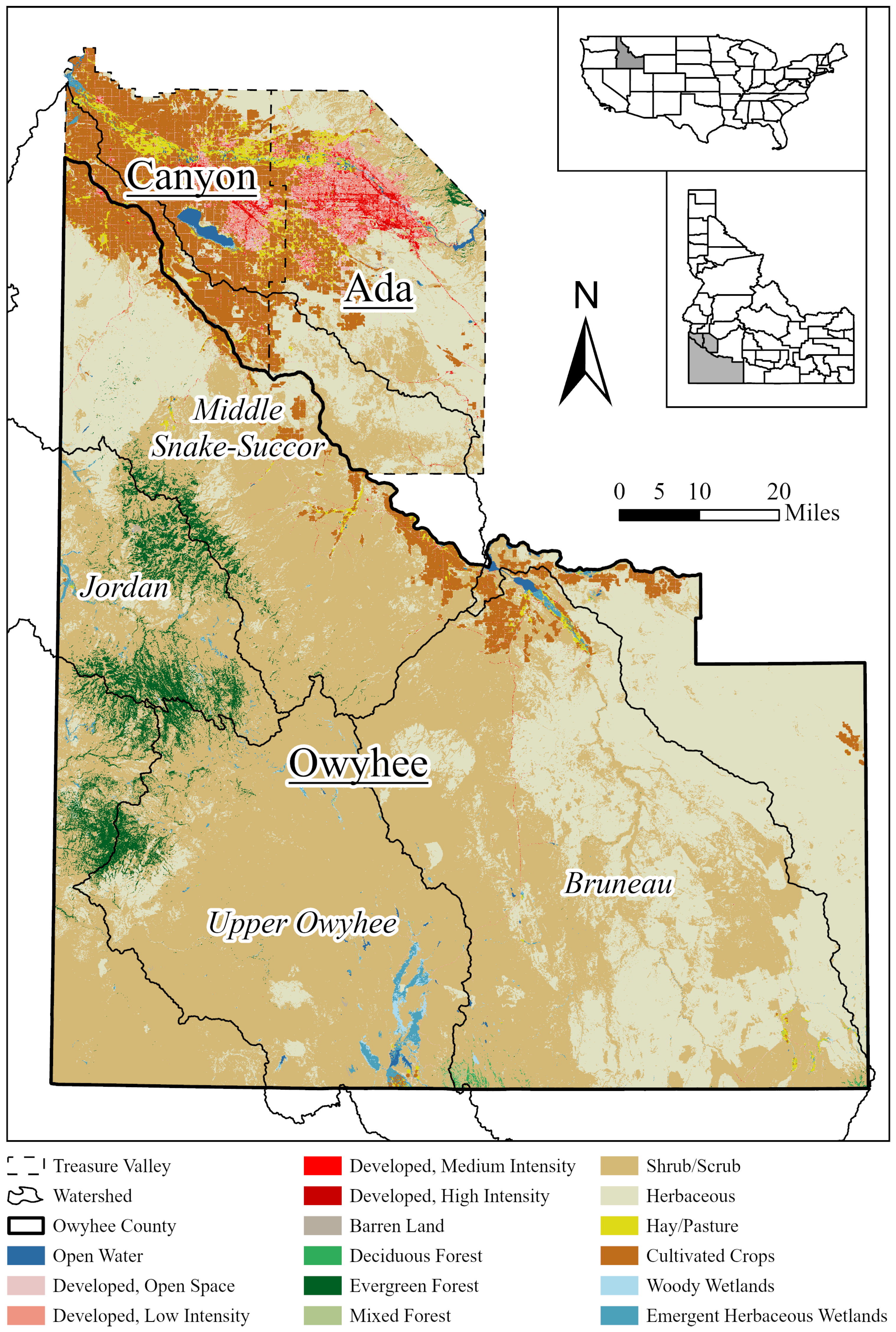
2.1. Study Area
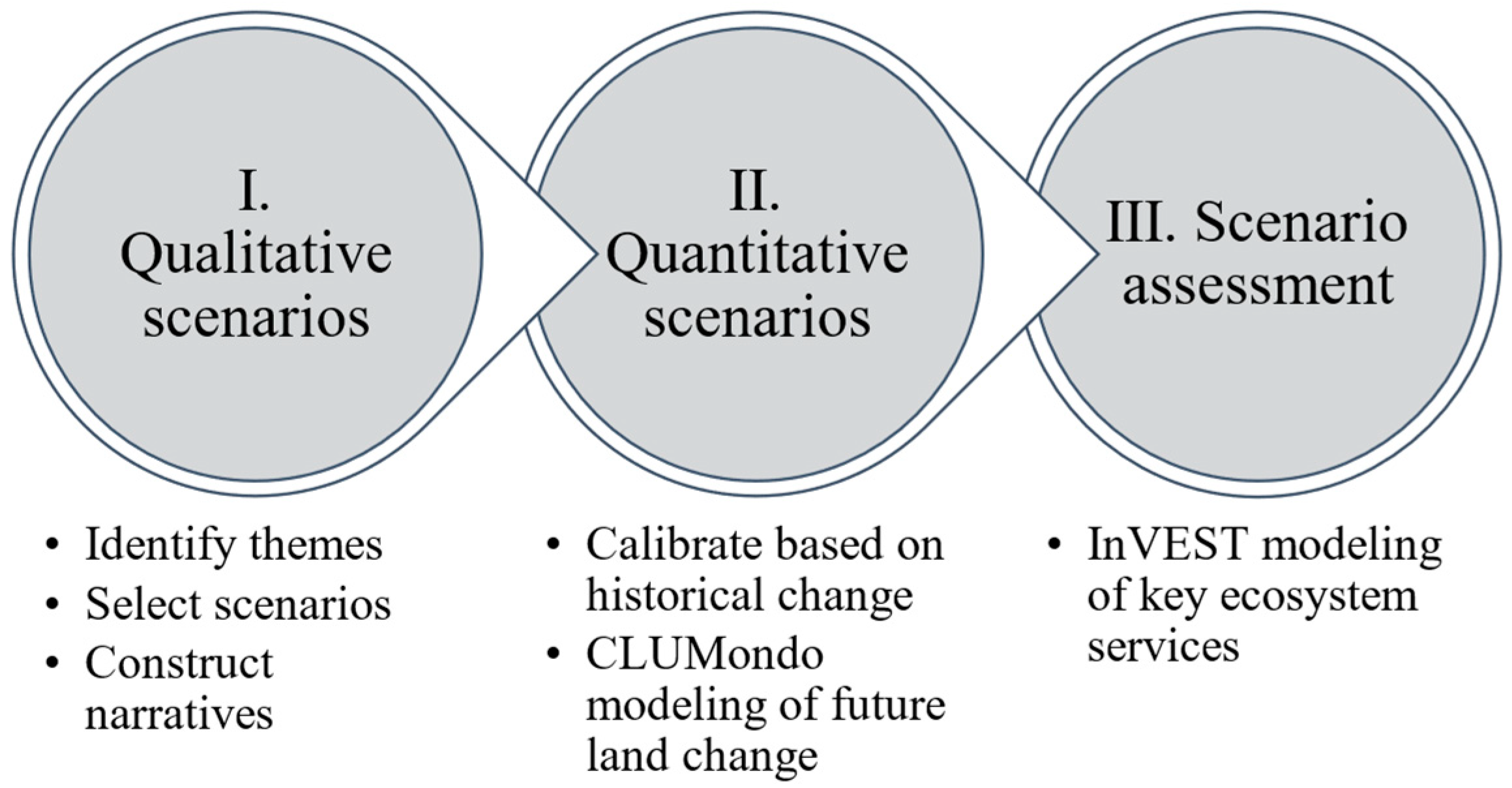
2.2. Overall Framework
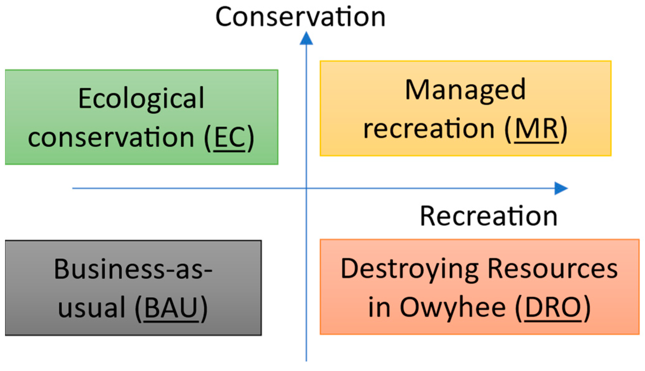
2.3. Qualitative Scenarios
2.4. Land System Scenarios by CLUMondo
2.5. Assessment of Ecosystem Services by InVEST
3. Results
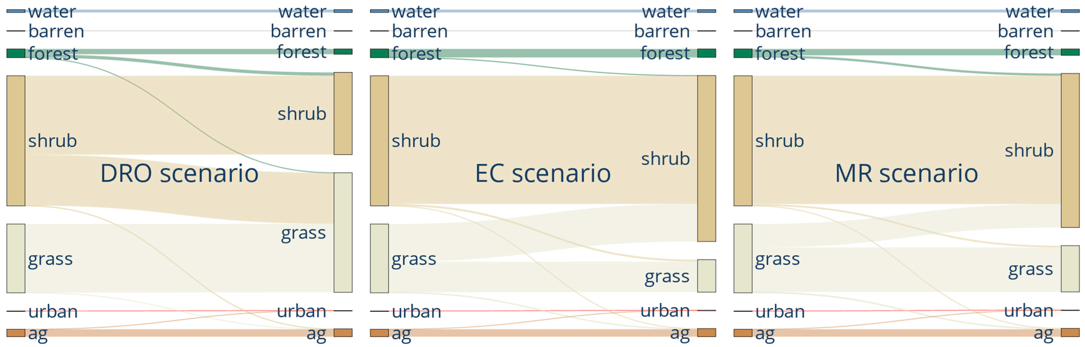
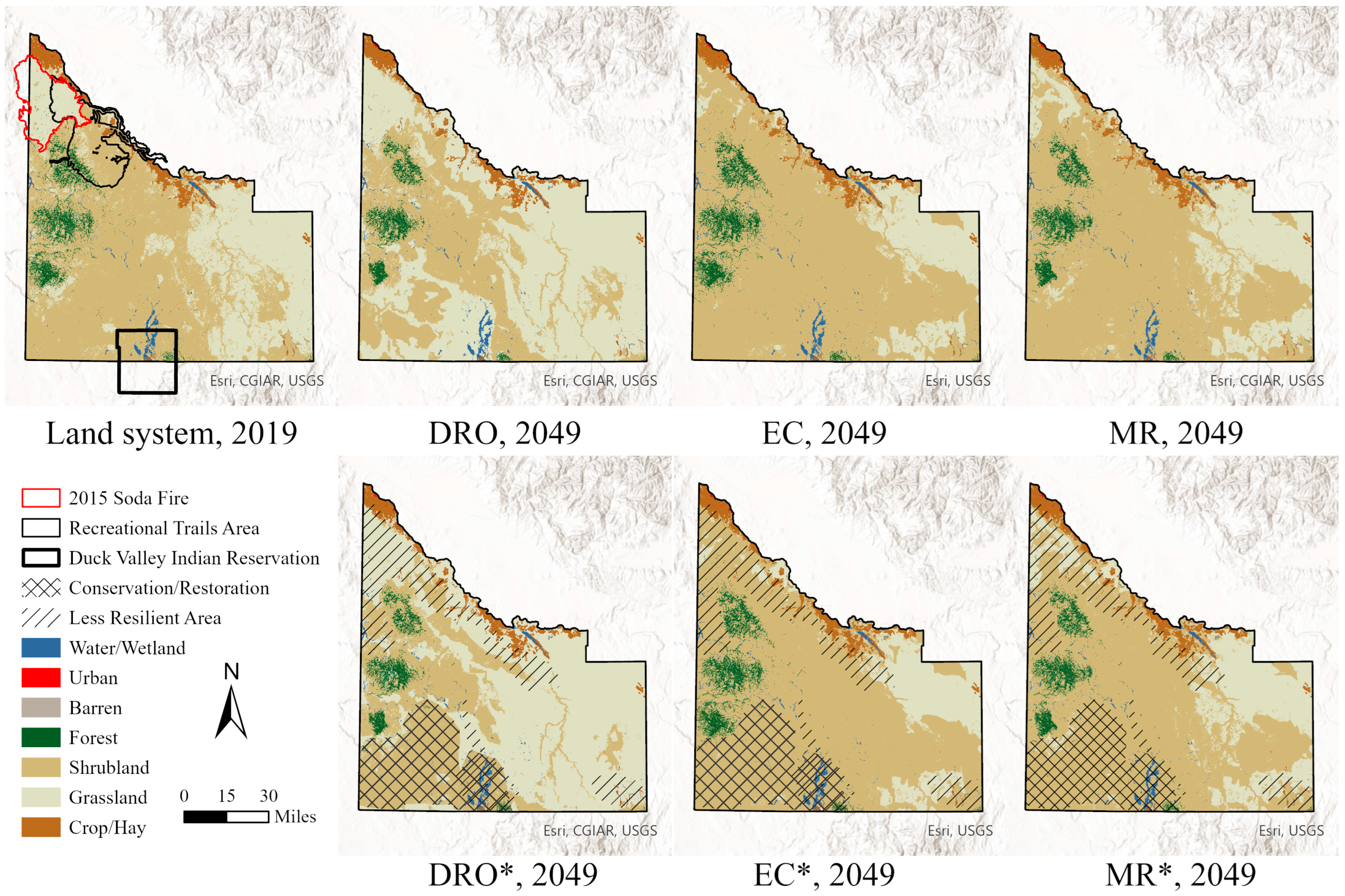
3.1. Land Systems and Rates of Change in Scenarios
3.2. Model Performance of CLUMondo and InVEST
3.3. Comparison of Land System Scenarios
3.4. Comparison of Environmental Impacts
4. Discussion
5. Limitations
6. Conclusions
Author Contributions
Funding
Institutional Review Board Statement
Informed Consent Statement
Data Availability Statement
Acknowledgments
Conflicts of Interest
Appendix A
- I.
- Scenario narratives (see [43])
- II.
- Appendix tables

| Decennial Change | From 2001 to 2011 | From 2011 to 2019 | From 2001 to 2019 |
|---|---|---|---|
| Urban | 9.40% | 6.81% | 8.54% |
| Sagebrush | −6.37% | −3.41% | −4.96% |
| EAG | 6.31% | 2.46% | 4.67% |
| Ag land | 4.06% | 2.08% | 3.22% |
| Abbreviation | Category | Variable | Description | Source |
|---|---|---|---|---|
| slope | Environmental | Slope (degree) | Calculated from elevation. | USDA NRCS |
| precip | Environmental | Precipitation (mm) | The 30 year normal annual precipitation, in milimeter. | PRISM Climate Group |
| popDen | Socioeconomic | Population density (1k/km2) | Calculated by census block population in 2010. | U.S. Census Bureau |
| mktAcc | Socioeconomic | Market accessibility (index from 0 to 1) | Access to national and international markets. | [86] |
| soilDep | Soil characteristics | Soil depth (cm) | Extracted from gNATSGO. | USDA NRCS |
| awc | Soil characteristics | Available water capacity (fraction) | Extracted from gNATSGO. | USDA NRCS |
| distUrban | Proximity | Distance to urban (km) | Calculated by distance to city/CDP in 2020. | U.S. Census Bureau |
| distRiver | Proximity | Distance to river (km) | Calculated by distance to rivers. | USGS |
| Coefficient * | Water | Urban | Barren | Forest | Shrub | Grass | Ag. Land |
|---|---|---|---|---|---|---|---|
| Constant | −5.7371 | −5.4721 | −9.5705 | −5.2821 | 3.4438 | −2.2986 | 2.1014 |
| slope | −0.5075 | −0.1594 | - | 0.0695 | 0.0024 | −0.0029 | −0.7561 |
| precip | 0.0028 | - | 0.0017 | 0.0109 | −0.0002 | −0.0067 | −0.0126 |
| popDen | −15.6612 | 10.1253 | - | −4381.2422 | −144.3840 | −79.6714 | −1.9413 |
| mktAcc | 1.4526 | 4.5171 | 8.4771 | −1.5294 | −0.4009 | −2.0504 | 6.2921 |
| soilDep | 0.0431 | - | 0.0199 | −0.0085 | −0.0174 | 0.0011 | - |
| awc | −3.2564 | - | −20.4530 | −15.7942 | −20.5207 | 23.8600 | 11.7380 |
| distUrban | −0.0056 | −0.0323 | - | - | 0.0104 | - | −0.0447 |
| distRiver | −0.0271 | −0.0800 | 0.0574 | −0.0611 | 0.0281 | 0.0048 | −0.0703 |
| AUC | 0.8319 | 0.9075 | 0.6363 | 0.9636 | 0.9012 | 0.7842 | 0.9610 |
| Land System | Water | Urban | Barren | Forest | Shrub | Grass | Ag Land |
|---|---|---|---|---|---|---|---|
| Value | 0.7 | 0.75 | 0.6 | 0.65 | 0.5 | 0.4 | 0.7 |
| Code | Class | Urban | Sagebrush | EAG | Ag Area |
|---|---|---|---|---|---|
| 0 | Water | 0 | 0 | 0 | 0 |
| 1 | Urban | 1 | 0 | 0 | 0 |
| 2 | Barren | 0 | 0 | 0 | 0 |
| 3 | Forest | 0 | 0 | 0 | 0 |
| 4 | Shrubland | 0 | 2 | 1 | 0 |
| 5 | Grassland | 0 | 1 | 2 | 0 |
| 7 | Ag. land | 0 | 0 | 0 | 1 |
| Code | Class | Water | Urban | Barren | Forest | Shrub | Grass | Ag. Land |
|---|---|---|---|---|---|---|---|---|
| 0 | Water | 1 | 0 | 0 | 0 | 0 | 0 | 0 |
| 1 | Urban | 0 | 1 | 0 | 0 | 0 | 0 | 0 |
| 2 | Barren | 0 | 0 | 1 | 0 | 0 | 0 | 0 |
| 3 | Forest | 0 | 0 | 0 | 1 | 1 | 1 | 0 |
| 4 | Shrubland | 0 | 0 | 0 | 1 | 1 | 1 | 1 |
| 5 | Grassland | 0 | 0 | 0 | 0 | 1 | 1 | 1 |
| 7 | Ag. land | 0 | 1 | 0 | 0 | 0 | 0 | 1 |
| Year | Location Accuracy | Pattern Accuracy | ||||||
|---|---|---|---|---|---|---|---|---|
| Misses | Hits | Wrong Hits | False Alarms | Correct Rejections | WPP | OMP | FIS | |
| 2011 | 2.43 | 8.72 | 0.01 | 2.75 | 86.09 | 97.18 | 94.81 | 78.14 |
| 2019 | 3.20 | 5.86 | 0.04 | 5.60 | 85.30 | 94.21 | 91.16 | 64.44 |
| Module | Data | Label | Source | Description |
|---|---|---|---|---|
| Annual water yield | Annual precipitation | PRISM; MACA | Historical data from the PRISM climate group, Oregon State University; future data from MACA dataset [102]. | |
| Available water content | STATSGO | The fraction of water in soil that is available to plants. | ||
| Z parameter | Calibration | The empirical constant typically ranges from 1 to 30. | ||
| Evapotranspiration coefficient | Literature; Calibration | Initial data from the literature [66,103]. | ||
| Reference evapotranspiration | PRISM; MACA | Calculated by the modified Hargreaves method [104]. | ||
| Water consumption | National Water-Use Science Project | Calculated by the county scale report [105]. | ||
| Sediment export | Rainfall erosivity | PRISM; MACA | Calculated by precipitation [76]. | |
| Soil erodibility | STATSGO | Soil’s susceptibility to detachment and transport by rainfall. | ||
| Slope length–gradient factor | NRCS | Calculated by terrain factors extracted from elevation [35]. | ||
| Cover-management factor | Literature; Calibration | Initial data from the literature [106,107]. | ||
| Support practice factor | Literature | Values from the literature [106,107]. | ||
| Maximum sediment retention ratio | Literature | Set to default value, 0.8 [79]. | ||
| Calibration parameter | Literature | Set to default value, 0.5 [79]. | ||
| Calibration parameter | Literature; Calibration | Initial data from the literature [79]. | ||
| Habitat quality | Habitat suitability | Literature | Values from the literature [108,109,110]. | |
| Relative sensitivity of LULC to threat | Literature | Values from the literature [108,109,110]. | ||
| Relative effect of threat | Literature | Values from the literature [108,109,110]. | ||
| Maximum effective distance of threat | Literature | Values from the literature [108,109,110]. |
- III.
- Spatial policies in the scenarios


| Scenario | Restriction | Locational Preference | |
|---|---|---|---|
| Grassland | Shrubland | ||
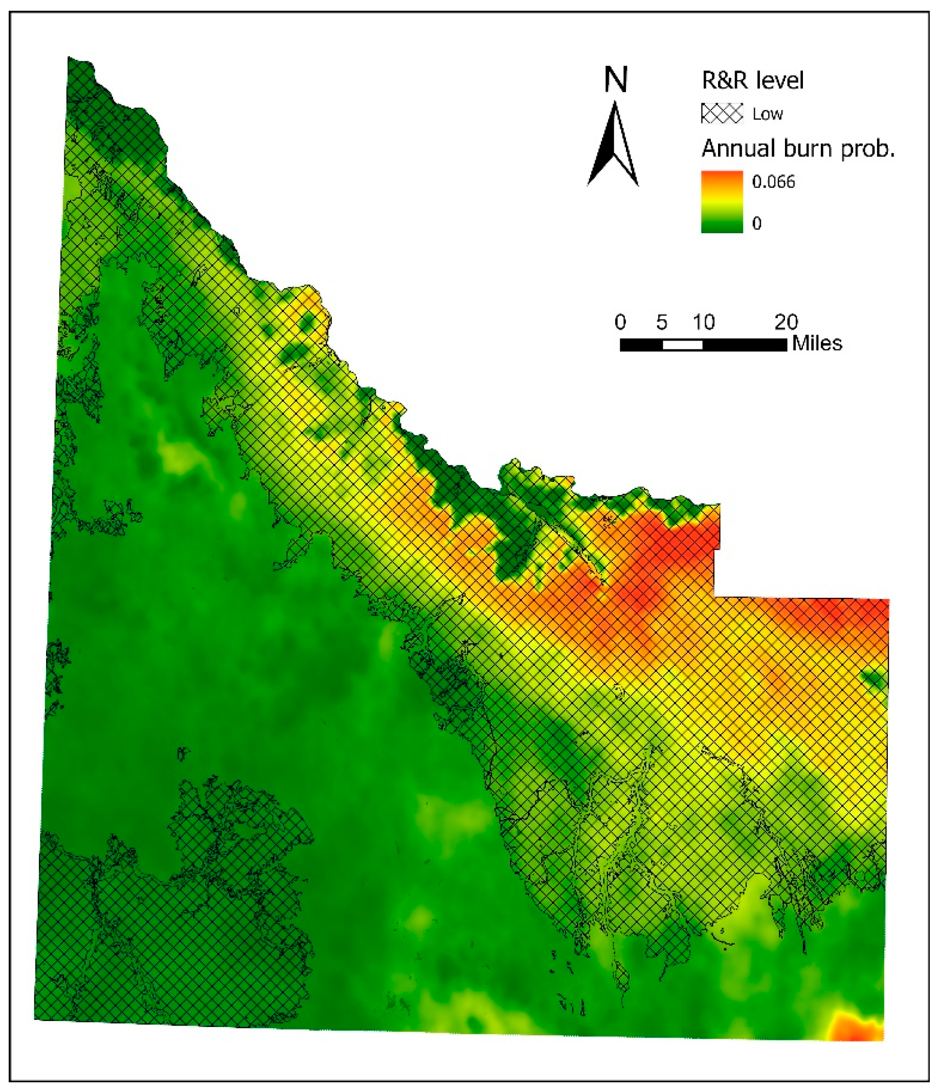
| BAU | - | Low R&R | - |
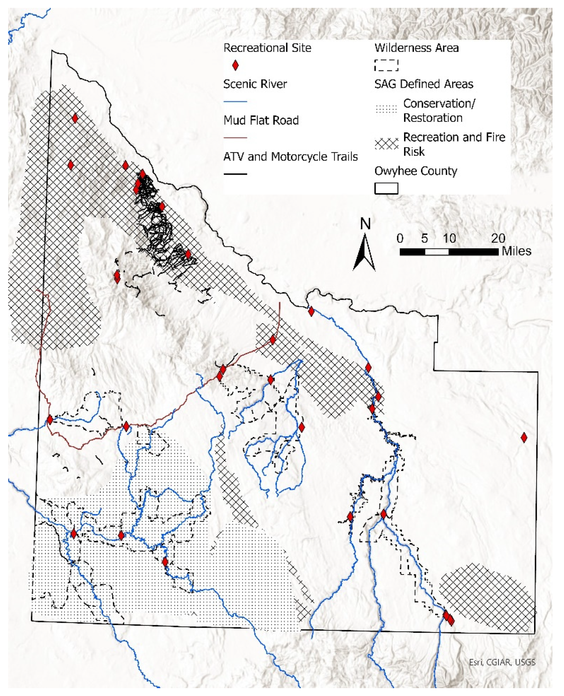
| DRO | Restoration/Conservation area defined by SAG | Low R&R; Rec. and Fire area by SAG and researchers | - |
| EC | - | Low R&R | Restoration/Conservation area defined by SAG; Rec. and Fire area by SAG and researchers |
| MR | - | Low R&R; Rec. and Fire area by SAG and researchers | Restoration/Conservation area defined by SAG |
References
- Van Asselen, S.; Verburg, P.H. A Land System Representation for Global Assessments and Land-Use Modeling. Glob. Chang. Biol. 2012, 18, 3125–3148. [Google Scholar] [CrossRef] [PubMed]
- Verburg, P.H.; Crossman, N.; Ellis, E.C.; Heinimann, A.; Hostert, P.; Mertz, O.; Nagendra, H.; Sikor, T.; Erb, K.-H.; Golubiewski, N.; et al. Land System Science and Sustainable Development of the Earth System: A Global Land Project Perspective. Anthropocene 2015, 12, 29–41. [Google Scholar] [CrossRef]
- Turner, B.L.; Lambin, E.F.; Verburg, P.H. From Land-Use/Land-Cover to Land System Science: This Article Belongs to Ambio’s 50th Anniversary Collection. Theme: Agricultural Land Use. Ambio 2021, 50, 1291–1294. [Google Scholar] [CrossRef] [PubMed]
- Meyfroidt, P.; de Bremond, A.; Ryan, C.M.; Archer, E.; Aspinall, R.; Chhabra, A.; Camara, G.; Corbera, E.; DeFries, R.; Díaz, S.; et al. Ten Facts about Land Systems for Sustainability. Proc. Natl. Acad. Sci. USA. 2022, 119, e2109217118. [Google Scholar] [CrossRef] [PubMed]
- Rounsevell, M.D.A.; Pedroli, B.; Erb, K.-H.; Gramberger, M.; Busck, A.G.; Haberl, H.; Kristensen, S.; Kuemmerle, T.; Lavorel, S.; Lindner, M.; et al. Challenges for Land System Science. Land Use Policy 2012, 29, 899–910. [Google Scholar] [CrossRef]
- Malek, Ž.; Verburg, P.H.; Geijzendorffer, I.R.; Bondeau, A.; Cramer, W. Global Change Effects on Land Management in the Mediterranean Region. Glob. Environ. Chang. 2018, 50, 238–254. [Google Scholar] [CrossRef]
- Martin, D.A.; Andrianisaina, F.; Fulgence, T.R.; Osen, K.; Rakotomalala, A.A.N.A.; Raveloaritiana, E.; Soazafy, M.R.; Wurz, A.; Andriafanomezantsoa, R.; Andriamaniraka, H.; et al. Land-Use Trajectories for Sustainable Land System Transformations: Identifying Leverage Points in a Global Biodiversity Hotspot. Proc. Natl. Acad. Sci. USA 2022, 119, e2107747119. [Google Scholar] [CrossRef]
- Sherrouse, B.C.; Semmens, D.J.; Ancona, Z.H.; Brunner, N.M. Analyzing Land-Use Change Scenarios for Trade-Offs among Cultural Ecosystem Services in the Southern Rocky Mountains. Ecosyst. Serv. 2017, 26, 431–444. [Google Scholar] [CrossRef]
- Hérivaux, C.; Vinatier, F.; Sabir, M.; Guillot, F.; Rinaudo, J.D. Combining Narrative Scenarios, Local Knowledge and Land-Use Change Modelling for Integrating Soil Erosion in a Global Perspective. Land Use Policy 2021, 105, 105406. [Google Scholar] [CrossRef]
- Navarro Garcia, J.; Marcos-Martinez, R.; Mosnier, A.; Schmidt-Traub, G.; Javalera Rincon, V.; Obersteiner, M.; Perez Guzman, K.; Thomson, M.J.; Penescu, L.; Douzal, C.; et al. Multi-Target Scenario Discovery to Plan for Sustainable Food and Land Systems in Australia. Sustain. Sci. 2023, 18, 371–388. [Google Scholar] [CrossRef]
- Thompson, J.R.; Plisinski, J.S.; Lambert, K.F.; Duveneck, M.J.; Morreale, L.; McBride, M.; MacLean, M.G.; Weiss, M.; Lee, L. Spatial Simulation of Codesigned Land Cover Change Scenarios in New England: Alternative Futures and Their Consequences for Conservation Priorities. Earth’s Future 2020, 8, e2019EF001348. [Google Scholar] [CrossRef]
- Cronan, D.; Trammell, E.J.; Kliskey, A.; Williams, P.; Alessa, L. Socio-Ecological Futures: Embedded Solutions for Stakeholder-Driven Alternative Futures. Sustainability 2022, 14, 3732. [Google Scholar] [CrossRef]
- McBride, M.F.; Lambert, K.F.; Huff, E.S.; Theoharides, K.A.; Field, P.; Thompson, J.R. Increasing the Effectiveness of Participatory Scenario Development through Codesign. Ecol. Soc. 2017, 22, 16. [Google Scholar] [CrossRef]
- Kliskey, A.; Williams, P.; Griffith, D.L.; Dale, V.H.; Schelly, C.; Marshall, A.-M.; Gagnon, V.S.; Eaton, W.M.; Floress, K. Thinking Big and Thinking Small: A Conceptual Framework for Best Practices in Community and Stakeholder Engagement in Food, Energy, and Water Systems. Sustainability 2021, 13, 2160. [Google Scholar] [CrossRef]
- Hölting, L.; Komossa, F.; Filyushkina, A.; Gastinger, M.-M.; Verburg, P.H.; Beckmann, M.; Volk, M.; Cord, A.F. Including Stakeholders’ Perspectives on Ecosystem Services in Multifunctionality Assessments. Ecosyst. People 2020, 16, 354–368. [Google Scholar] [CrossRef]
- Kim, Y.; Newman, G.; Güneralp, B. A Review of Driving Factors, Scenarios, and Topics in Urban Land Change Models. Land 2020, 9, 246. [Google Scholar] [CrossRef]
- Gourguet, S.; Marzloff, M.P.; Bacher, C.; Boudry, P.; Cugier, P.; Dambacher, J.M.; Desroy, N.; Gangnery, A.; Le Mao, P.; Monnier, L.; et al. Participatory Qualitative Modeling to Assess the Sustainability of a Coastal Socio-Ecological System. Front. Ecol. Evol. 2021, 9, 635857. [Google Scholar] [CrossRef]
- Salliou, N.; Barnaud, C.; Vialatte, A.; Monteil, C. A Participatory Bayesian Belief Network Approach to Explore Ambiguity among Stakeholders about Socio-Ecological Systems. Environ. Modell. Softw. 2017, 96, 199–209. [Google Scholar] [CrossRef]
- De Stefano, L.; Hernández-Mora, N.; Iglesias, A.; Sánchez, B. Defining Adaptation Measures Collaboratively: A Participatory Approach in the Doñana Socio-Ecological System, Spain. J. Environ. Manag. 2017, 195, 46–55. [Google Scholar] [CrossRef]
- Allan, A.; Barbour, E.; Nicholls, R.J.; Hutton, C.; Lim, M.; Salehin, M.; Rahman, M.M. Developing Socio-Ecological Scenarios: A Participatory Process for Engaging Stakeholders. Sci. Total Environ. 2022, 807, 150512. [Google Scholar] [CrossRef]
- Capitani, C.; Garedew, W.; Mitiku, A.; Berecha, G.; Hailu, B.T.; Heiskanen, J.; Hurskainen, P.; Platts, P.J.; Siljander, M.; Pinard, F.; et al. Views from Two Mountains: Exploring Climate Change Impacts on Traditional Farming Communities of Eastern Africa Highlands through Participatory Scenarios. Sustain. Sci. 2019, 14, 191–203. [Google Scholar] [CrossRef]
- Kabaya, K.; Hashimoto, S.; Fukuyo, N.; Uetake, T.; Takeuchi, K. Investigating Future Ecosystem Services through Participatory Scenario Building and Spatial Ecological–Economic Modelling. Sustain. Sci. 2019, 14, 77–88. [Google Scholar] [CrossRef]
- Reed, M.S.; Kenter, J.; Bonn, A.; Broad, K.; Burt, T.P.; Fazey, I.R.; Fraser, E.D.G.; Hubacek, K.; Nainggolan, D.; Quinn, C.H.; et al. Participatory Scenario Development for Environmental Management: A Methodological Framework Illustrated with Experience from the UK Uplands. J. Environ. Manag. 2013, 128, 345–362. [Google Scholar] [CrossRef] [PubMed]
- Esgalhado, C.; Guimarães, M.H.; Lardon, S.; Debolini, M.; Balzan, M.V.; Gennai-Schott, S.C.; Simón Rojo, M.; Mekki, I.; Bouchemal, S. Mediterranean Land System Dynamics and Their Underlying Drivers: Stakeholder Perception from Multiple Case Studies. Landsc. Urban Plan. 2021, 213, 104134. [Google Scholar] [CrossRef]
- Russeil, V.; Lo Seen, D.; Broust, F.; Bonin, M.; Praene, J.-P. Food and Electricity Self-Sufficiency Trade-Offs in Reunion Island: Modelling Land-Use Change Scenarios with Stakeholders. Land Use Policy 2023, 132, 106784. [Google Scholar] [CrossRef]
- Mahmoud, M.; Liu, Y.; Hartmann, H.; Stewart, S.; Wagener, T.; Semmens, D.; Stewart, R.; Gupta, H.; Dominguez, D.; Dominguez, F.; et al. A Formal Framework for Scenario Development in Support of Environmental Decision-Making. Environ. Model. Softw. 2009, 24, 798–808. [Google Scholar] [CrossRef]
- Mallampalli, V.R.; Mavrommati, G.; Thompson, J.; Duveneck, M.; Meyer, S.; Ligmann-Zielinska, A.; Druschke, C.G.; Hychka, K.; Kenney, M.A.; Kok, K. Methods for Translating Narrative Scenarios into Quantitative Assessments of Land Use Change. Environ. Model. Softw. 2016, 82, 7–20. [Google Scholar] [CrossRef]
- Kliskey, A.A.; Williams, P.; Trammell, E.J.; Cronan, D.; Griffith, D.; Alessa, L.; Lammers, R.; de Haro-Martí, M.E.; Oxarango-Ingram, J. Building Trust, Building Futures: Knowledge Co-Production as Relationship, Design, and Process in Transdisciplinary Science. Front. Environ. Sci. 2023, 11, 1007105. [Google Scholar] [CrossRef]
- Delmotte, S.; Couderc, V.; Mouret, J.-C.; Lopez-Ridaura, S.; Barbier, J.-M.; Hossard, L. From Stakeholders Narratives to Modelling Plausible Future Agricultural Systems. Integrated Assessment of Scenarios for Camargue, Southern France. Eur. J. Agron. 2017, 82, 292–307. [Google Scholar] [CrossRef]
- Duguma, D.; Schultner, J.; Abson, D.; Fischer, J. From Stories to Maps: Translating Participatory Scenario Narratives into Spatially Explicit Information. Ecol. Soc. 2022, 27, 13. [Google Scholar] [CrossRef]
- Proswitz, K.; Edward, M.C.; Evers, M.; Mombo, F.; Mpwaga, A.; Näschen, K.; Sesabo, J.; Höllermann, B. Complex Socio-Ecological Systems: Translating Narratives into Future Land Use and Land Cover Scenarios in the Kilombero Catchment, Tanzania. Sustainability 2021, 13, 6552. [Google Scholar] [CrossRef]
- Bayala, E.R.C.; Asubonteng, K.O.; Ros-Tonen, M.; Djoudi, H.; Siangulube, F.S.; Reed, J.; Sunderland, T. Using Scenario Building and Participatory Mapping to Negotiate Conservation-Development Trade-Offs in Northern Ghana. Land 2023, 12, 580. [Google Scholar] [CrossRef]
- Wulfhorst, J.D.; Rimbey, N.; Darden, T. Sharing the Rangelands, Competing for Sense of Place. Am. Behav. Sci. 2006, 50, 166–186. [Google Scholar] [CrossRef]
- Van Asselen, S.; Verburg, P.H. Land Cover Change or Land-Use Intensification: Simulating Land System Change with a Global-Scale Land Change Model. Glob. Chang. Biol. 2013, 19, 3648–3667. [Google Scholar] [CrossRef] [PubMed]
- InVEST 3.14.0. Available online: https://naturalcapitalproject.stanford.edu/software/invest (accessed on 15 November 2023).
- Brymer, A.L.B.; Holbrook, J.D.; Niemeyer, R.J.; Suazo, A.A.; Wulfhorst, J.D.; Vierling, K.T.; Newingham, B.A.; Link, T.E.; Rachlow, J.L. A Social-Ecological Impact Assessment for Public Lands Management: Application of a Conceptual and Methodological Framework. Ecol. Soc. 2016, 21, 9. [Google Scholar] [CrossRef]
- Dahal, K.R.; Benner, S.; Lindquist, E. Urban Hypotheses and Spatiotemporal Characterization of Urban Growth in the Treasure Valley of Idaho, USA. Appl. Geogr. 2017, 79, 11–25. [Google Scholar] [CrossRef]
- Brymer, A.L.B.; Wulfhorst, J.D.; Brunson, M.W. Analyzing Stakeholders’ Workshop Dialogue for Evidence of Social Learning. Ecol. Soc. 2018, 23, 42. [Google Scholar] [CrossRef]
- Coates, P.S.; Ricca, M.A.; Prochazka, B.G.; Brooks, M.L.; Doherty, K.E.; Kroger, T.; Blomberg, E.J.; Hagen, C.A.; Casazza, M.L. Wildfire, Climate, and Invasive Grass Interactions Negatively Impact an Indicator Species by Reshaping Sagebrush Ecosystems. Proc. Natl. Acad. Sci. USA 2016, 113, 12745–12750. [Google Scholar] [CrossRef]
- Hamilton, S.H.; ElSawah, S.; Guillaume, J.H.A.; Jakeman, A.J.; Pierce, S.A. Integrated Assessment and Modelling: Overview and Synthesis of Salient Dimensions. Environ. Model. Softw. 2015, 64, 215–229. [Google Scholar] [CrossRef]
- Yin, L.; Zhang, S.; Zhang, B. Do Ecological Restoration Projects Improve Water-Related Ecosystem Services? Evidence from a Study in the Hengduan Mountain Region. Int. J. Environ. Res. Public Health 2022, 19, 3860. [Google Scholar] [CrossRef]
- Nie, X.; Lu, B.; Chen, Z.; Yang, Y.; Chen, S.; Chen, Z.; Wang, H. Increase or Decrease? Integrating the CLUMondo and InVEST Models to Assess the Impact of the Implementation of the Major Function Oriented Zone Planning on Carbon Storage. Ecol. Indic. 2020, 118, 106708. [Google Scholar] [CrossRef]
- Cronan, D.; Huang, L.; Kliskey, A.; Zinzer, B.; Burnham, M.; Griswald, K.; Ebel, S.; Hopping, K.; Fredeluces-Hart, G. Alternative Futures for Southern Idaho: Landscape Trajectories of Change for the Owyhee Region and Teton Valley. Front. Environ. Sci. 2024; in preparation. [Google Scholar]
- Ornetsmüller, C.; Verburg, P.H.; Heinimann, A. Scenarios of Land System Change in the Lao PDR: Transitions in Response to Alternative Demands on Goods and Services Provided by the Land. Appl. Geogr. 2016, 75, 1–11. [Google Scholar] [CrossRef]
- Edrisi, S.A.; Bundela, A.K.; Verma, V.; Dubey, P.K.; Abhilash, P.C. Assessing the Impact of Global Initiatives on Current and Future Land Restoration Scenarios in India. Environ. Res. 2023, 216, 114413. [Google Scholar] [CrossRef] [PubMed]
- Domingo, D.; Palka, G.; Hersperger, A.M. Effect of Zoning Plans on Urban Land-Use Change: A Multi-Scenario Simulation for Supporting Sustainable Urban Growth. Sustain. Cities Soc. 2021, 69, 102833. [Google Scholar] [CrossRef]
- Bacău, S.; Domingo, D.; Palka, G.; Pellissier, L.; Kienast, F. Integrating Strategic Planning Intentions into Land-Change Simulations: Designing and Assessing Scenarios for Bucharest. Sustain. Cities Soc. 2022, 76, 103446. [Google Scholar] [CrossRef]
- Cronan, D.; Trammell, E.J.; Kliskey, A. Images to Evoke Decision-Making: Building Compelling Representations for Stakeholder-Driven Futures. Sustainability 2022, 14, 2980. [Google Scholar] [CrossRef]
- Gomes, E.; Inácio, M.; Bogdzevič, K.; Kalinauskas, M.; Karnauskaitė, D.; Pereira, P. Future Land-Use Changes and Its Impacts on Terrestrial Ecosystem Services: A Review. Sci. Total Environ. 2021, 781, 146716. [Google Scholar] [CrossRef]
- Rowe, G.; Wright, G. The Delphi Technique as a Forecasting Tool: Issues and Analysis. Int. J. Forecast. 1999, 15, 353–375. [Google Scholar] [CrossRef]
- Jin, X.; Jiang, P.; Ma, D.; Li, M. Land System Evolution of Qinghai-Tibetan Plateau under Various Development Strategies. Appl. Geogr. 2019, 104, 1–9. [Google Scholar] [CrossRef]
- Malek, Ž.; Verburg, P.H. Adaptation of Land Management in the Mediterranean under Scenarios of Irrigation Water Use and Availability. Mitig. Adapt. Strat. Glob. Chang. 2018, 23, 821–837. [Google Scholar] [CrossRef] [PubMed]
- Wang, C.; Yu, C.; Chen, T.; Feng, Z.; Hu, Y.; Wu, K. Can the Establishment of Ecological Security Patterns Improve Ecological Protection? An Example of Nanchang, China. Sci. Total Environ. 2020, 740, 140051. [Google Scholar] [CrossRef] [PubMed]
- Wang, Y.; van Vliet, J.; Debonne, N.; Pu, L.; Verburg, P.H. Settlement Changes after Peak Population: Land System Projections for China until 2050. Landsc. Urban Plan. 2021, 209, 104045. [Google Scholar] [CrossRef]
- Wu, J.; Jin, X.; Feng, Z.; Chen, T.; Wang, C.; Feng, D.; Lv, J. Relationship of Ecosystem Services in the Beijing–Tianjin–Hebei Region Based on the Production Possibility Frontier. Land 2021, 10, 881. [Google Scholar] [CrossRef]
- Zhu, W.; Gao, Y.; Zhang, H.; Liu, L. Optimization of the Land Use Pattern in Horqin Sandy Land by Using the CLUMondo Model and Bayesian Belief Network. Sci. Total Environ. 2020, 739, 139929. [Google Scholar] [CrossRef] [PubMed]
- Gao, P.; Gao, Y.; Zhang, X.; Ye, S.; Song, C. CLUMondo-BNU for Simulating Land System Changes Based on Many-to-Many Demand–Supply Relationships with Adaptive Conversion Orders. Sci. Rep. 2023, 13, 5559. [Google Scholar] [CrossRef]
- Arunyawat, S.; Shrestha, R.P. Simulating Future Land Use and Ecosystem Services in Northern Thailand. J. Land Use Sci. 2018, 13, 146–165. [Google Scholar] [CrossRef]
- Pontius, R.G.; Boersma, W.; Castella, J.-C.; Clarke, K.; de Nijs, T.; Dietzel, C.; Duan, Z.; Fotsing, E.; Goldstein, N.; Kok, K.; et al. Comparing the Input, Output, and Validation Maps for Several Models of Land Change. Ann. Reg. Sci 2008, 42, 11–37. [Google Scholar] [CrossRef]
- Power, C.; Simms, A.; White, R. Hierarchical Fuzzy Pattern Matching for the Regional Comparison of Land Use Maps. Int. J. Geogr. Inf. Sci. 2001, 15, 77–100. [Google Scholar] [CrossRef]
- Yin, L.; Dai, E.; Xie, G.; Zhang, B. Effects of Land-Use Intensity and Land Management Policies on Evolution of Regional Land System: A Case Study in the Hengduan Mountain Region. Land 2021, 10, 528. [Google Scholar] [CrossRef]
- Zhao, Y.; Wang, M.; Lan, T.; Xu, Z.; Wu, J.; Liu, Q.; Peng, J. Distinguishing the Effects of Land Use Policies on Ecosystem Services and Their Trade-Offs Based on Multi-Scenario Simulations. Appl. Geogr. 2023, 151, 102864. [Google Scholar] [CrossRef]
- Gu, Y.; Deal, B.; Larsen, L. Geodesign Processes and Ecological Systems Thinking in a Coupled Human-Environment Context: An Integrated Framework for Landscape Architecture. Sustainability 2018, 10, 3306. [Google Scholar] [CrossRef]
- Gomes, L.C.; Bianchi, F.J.J.A.; Cardoso, I.M.; Schulte, R.P.O.; Arts, B.J.M.; Fernandes Filho, E.I. Land Use and Land Cover Scenarios: An Interdisciplinary Approach Integrating Local Conditions and the Global Shared Socioeconomic Pathways. Land Use Policy 2020, 97, 104723. [Google Scholar] [CrossRef]
- Gao, J.; Li, F.; Gao, H.; Zhou, C.; Zhang, X. The Impact of Land-Use Change on Water-Related Ecosystem Services: A Study of the Guishui River Basin, Beijing, China. J. Clean. Prod. 2017, 163, S148–S155. [Google Scholar] [CrossRef]
- Huang, L.; Liao, F.H.; Lohse, K.A.; Larson, D.M.; Fragkias, M.; Lybecker, D.L.; Baxter, C.V. Land Conservation Can Mitigate Freshwater Ecosystem Services Degradation Due to Climate Change in a Semiarid Catchment: The Case of the Portneuf River Catchment, Idaho, USA. Sci. Total Environ. 2019, 651, 1796–1809. [Google Scholar] [CrossRef] [PubMed]
- Kusi, K.K.; Khattabi, A.; Mhammdi, N.; Lahssini, S. Prospective Evaluation of the Impact of Land Use Change on Ecosystem Services in the Ourika Watershed, Morocco. Land Use Policy 2020, 97, 104796. [Google Scholar] [CrossRef]
- Li, Z.; Cheng, X.; Han, H. Analyzing Land-Use Change Scenarios for Ecosystem Services and Their Trade-Offs in the Ecological Conservation Area in Beijing, China. Int. J. Environ. Res. Public Health 2020, 17, 8632. [Google Scholar] [CrossRef]
- Wu, Y.; Tao, Y.; Yang, G.; Ou, W.; Pueppke, S.; Sun, X.; Chen, G.; Tao, Q. Impact of Land Use Change on Multiple Ecosystem Services in the Rapidly Urbanizing Kunshan City of China: Past Trajectories and Future Projections. Land Use Policy 2019, 85, 419–427. [Google Scholar] [CrossRef]
- Yang, S.; Zhao, W.; Liu, Y.; Wang, S.; Wang, J.; Zhai, R. Influence of Land Use Change on the Ecosystem Service Trade-Offs in the Ecological Restoration Area: Dynamics and Scenarios in the Yanhe Watershed, China. Sci. Total Environ. 2018, 644, 556–566. [Google Scholar] [CrossRef]
- Xu, J.; Renaud, F.G.; Barrett, B. Modelling Land System Evolution and Dynamics of Terrestrial Carbon Stocks in the Luanhe River Basin, China: A Scenario Analysis of Trade-Offs and Synergies between Sustainable Development Goals. Sustain. Sci. 2022, 17, 1323–1345. [Google Scholar] [CrossRef]
- Zhang, L.; Hickel, K.; Dawes, W.; Chiew, F.H.; Western, A.; Briggs, P. A Rational Function Approach for Estimating Mean Annual Evapotranspiration. Water Resour. Res. 2004, 40, W02502. [Google Scholar] [CrossRef]
- Donohue, R.J.; Roderick, M.L.; McVicar, T.R. Roots, Storms and Soil Pores: Incorporating Key Ecohydrological Processes into Budyko’s Hydrological Model. J. Hydrol. 2012, 436, 35–50. [Google Scholar] [CrossRef]
- Zhang, L.; Dawes, W.; Walker, G. Response of Mean Annual Evapotranspiration to Vegetation Changes at Catchment Scale. Water Resour. Res. 2001, 37, 701–708. [Google Scholar] [CrossRef]
- Hamel, P.; Chaplin-Kramer, R.; Sim, S.; Mueller, C. A New Approach to Modeling the Sediment Retention Service (InVEST 3.0): Case Study of the Cape Fear Catchment, North Carolina, USA. Sci. Total Environ. 2015, 524, 166–177. [Google Scholar] [CrossRef] [PubMed]
- Renard, K.G.; Freimund, J.R. Using Monthly Precipitation Data to Estimate the R-Factor in the Revised USLE. J. Hydrol. 1994, 157, 287–306. [Google Scholar] [CrossRef]
- Sanchez, A.; Malak, D.A.; Guelmami, A.; Perennou, C. Development of an Indicator to Monitor Mediterranean Wetlands. PLoS ONE 2015, 10, e0122694. [Google Scholar] [CrossRef] [PubMed]
- Borselli, L.; Cassi, P.; Torri, D. Prolegomena to Sediment and Flow Connectivity in the Landscape: A GIS and Field Numerical Assessment. CATENA 2008, 75, 268–277. [Google Scholar] [CrossRef]
- Vigiak, O.; Borselli, L.; Newham, L.; McInnes, J.; Roberts, A. Comparison of Conceptual Landscape Metrics to Define Hillslope-Scale Sediment Delivery Ratio. Geomorphology 2012, 138, 74–88. [Google Scholar] [CrossRef]
- Pastick, N.J.; Wylie, B.K.; Rigge, M.B.; Dahal, D.; Boyte, S.P.; Jones, M.O.; Allred, B.W.; Parajuli, S.; Wu, Z. Rapid Monitoring of the Abundance and Spread of Exotic Annual Grasses in the Western United States Using Remote Sensing and Machine Learning. AGU Adv. 2021, 2, e2020AV000298. [Google Scholar] [CrossRef]
- Shi, H.; Rigge, M.; Postma, K.; Bunde, B. Trends Analysis of Rangeland Condition Monitoring Assessment and Projection (RCMAP) Fractional Component Time Series (1985–2020). GISci. Remote Sens. 2022, 59, 1243–1265. [Google Scholar] [CrossRef]
- Pontius, R.G.; Spencer, J. Uncertainty in Extrapolations of Predictive Land-Change Models. Environ. Plan. B Plan. Des. 2005, 32, 211–230. [Google Scholar] [CrossRef]
- Deb, K.; Pratap, A.; Agarwal, S.; Meyarivan, T. A Fast and Elitist Multiobjective Genetic Algorithm: NSGA-II. IEEE Trans. Evol. Comput. 2002, 6, 182–197. [Google Scholar] [CrossRef]
- Kling, H.; Fuchs, M.; Paulin, M. Runoff Conditions in the Upper Danube Basin under an Ensemble of Climate Change Scenarios. J. Hydrol. 2012, 424–425, 264–277. [Google Scholar] [CrossRef]
- Nash, J.E.; Sutcliffe, J.V. River Flow Forecasting through Conceptual Models Part I—A Discussion of Principles. J. Hydrol. 1970, 10, 282–290. [Google Scholar] [CrossRef]
- Kliskey, A.; Abatzoglou, J.; Alessa, L.; Kolden, C.; Hoekema, D.; Moore, B.; Gilmore, S.; Austin, G. Planning for Idaho’s Waterscapes: A Review of Historical Drivers and Outlook for the next 50 Years. Environ. Sci. Policy 2019, 94, 191–201. [Google Scholar] [CrossRef]
- Do, T.H.; Vu, T.P.; Catacutan, D.; Nguyen, V.T. Governing Landscapes for Ecosystem Services: A Participatory Land-Use Scenario Development in the Northwest Montane Region of Vietnam. Environ. Manag. 2021, 68, 665–682. [Google Scholar] [CrossRef] [PubMed]
- Gullino, P.; Mellano, M.G.; Beccaro, G.L.; Devecchi, M.; Larcher, F. Strategies for the Management of Traditional Chestnut Landscapes in Pesio Valley, Italy: A Participatory Approach. Land 2020, 9, 536. [Google Scholar] [CrossRef]
- Sahraoui, Y.; De Godoy Leski, C.; Benot, M.-L.; Revers, F.; Salles, D.; van Halder, I.; Barneix, M.; Carassou, L. Integrating Ecological Networks Modelling in a Participatory Approach for Assessing Impacts of Planning Scenarios on Landscape Connectivity. Landsc. Urban Plan. 2021, 209, 104039. [Google Scholar] [CrossRef]
- Iwaniec, D.M.; Cook, E.M.; Davidson, M.J.; Berbés-Blázquez, M.; Georgescu, M.; Krayenhoff, E.S.; Middel, A.; Sampson, D.A.; Grimm, N.B. The Co-Production of Sustainable Future Scenarios. Landsc. Urban Plan. 2020, 197, 103744. [Google Scholar] [CrossRef]
- Brymer, A.L.B.; Toledo, D.; Spiegal, S.; Pierson, F.; Clark, P.E.; Wulfhorst, J.D. Social-Ecological Processes and Impacts Affect Individual and Social Well-Being in a Rural Western U.S. Landscape. Front. Sustain. Food Syst. 2020, 4, 38. [Google Scholar] [CrossRef]
- Meyfroidt, P.; Roy Chowdhury, R.; de Bremond, A.; Ellis, E.C.; Erb, K.-H.; Filatova, T.; Garrett, R.D.; Grove, J.M.; Heinimann, A.; Kuemmerle, T.; et al. Middle-Range Theories of Land System Change. Glob. Environ. Chang. 2018, 53, 52–67. [Google Scholar] [CrossRef]
- Busck-Lumholt, L.M.; Coenen, J.; Persson, J.; Frohn Pedersen, A.; Mertz, O.; Corbera, E. Telecoupling as a Framework to Support a More Nuanced Understanding of Causality in Land System Science. J. Land Use Sci. 2022, 17, 386–406. [Google Scholar] [CrossRef]
- Hull, V.; Liu, J. Telecoupling: A New Frontier for Global Sustainability. Ecol. Soc. 2018, 23, 41. [Google Scholar] [CrossRef]
- Huang, L.; Cronan, D.; Kliskey, A. Modeling of Landscape Change and Tele-Coupling in Local Socio-Ecological Systems: A Simulation of Land Use Change and Recreational Activities in Southern Idaho, United States. In Proceedings of the 2021 Annual Modeling and Simulation Conference (ANNSIM), Online, 19–22 July 2021; IEEE: Piscataway, NJ, USA, 2021; pp. 1–12. [Google Scholar]
- Moroney, J.L.; Castellano, R.S. Farmland Loss and Concern in the Treasure Valley. Agric. Hum. Values 2018, 35, 529–536. [Google Scholar] [CrossRef]
- Larson, C.D.; Lehnhoff, E.A.; Rew, L.J. A Warmer and Drier Climate in the Northern Sagebrush Biome Does Not Promote Cheatgrass Invasion or Change Its Response to Fire. Oecologia 2017, 185, 763–774. [Google Scholar] [CrossRef] [PubMed]
- Wickham, J.; Stehman, S.V.; Sorenson, D.G.; Gass, L.; Dewitz, J.A. Thematic Accuracy Assessment of the NLCD 2019 Land Cover for the Conterminous United States. GISci. Remote Sens. 2023, 60, 2181143. [Google Scholar] [CrossRef]
- Rupp, D.E.; Abatzoglou, J.T.; Hegewisch, K.C.; Mote, P.W. Evaluation of CMIP5 20th Century Climate Simulations for the Pacific Northwest USA. J. Geophys. Res. Atmos. 2013, 118, 10884–10906. [Google Scholar] [CrossRef]
- Hamel, P.; Bryant, B.P. Uncertainty Assessment in Ecosystem Services Analyses: Seven Challenges and Practical Responses. Ecosyst. Serv. 2017, 24, 1–15. [Google Scholar] [CrossRef]
- Rounsevell, M.D.A.; Arneth, A.; Brown, C.; Cheung, W.W.L.; Gimenez, O.; Holman, I.; Leadley, P.; Luján, C.; Mahevas, S.; Maréchaux, I.; et al. Identifying Uncertainties in Scenarios and Models of Socio-Ecological Systems in Support of Decision-Making. One Earth 2021, 4, 967–985. [Google Scholar] [CrossRef]
- Abatzoglou, J.T.; Brown, T.J. A Comparison of Statistical Downscaling Methods Suited for Wildfire Applications. Int. J. Climatol. 2012, 32, 772–780. [Google Scholar] [CrossRef]
- Hoyer, R.; Chang, H. Assessment of Freshwater Ecosystem Services in the Tualatin and Yamhill Basins under Climate Change and Urbanization. Appl. Geogr. 2014, 53, 402–416. [Google Scholar] [CrossRef]
- Droogers, P.; Allen, R.G. Estimating Reference Evapotranspiration Under Inaccurate Data Conditions. Irrig. Drain. Syst. 2002, 16, 33–45. [Google Scholar] [CrossRef]
- Dieter, C.A.; Maupin, M.A.; Caldwell, R.R.; Harris, M.A.; Ivahnenko, T.I.; Lovelace, J.K.; Barber, N.L.; Linsey, K.S. Estimated Use of Water in the United States in 2015; Circular; US Geological Survey: Reston, VA, USA, 2018. [Google Scholar]
- Fernandez, C.; Wu, J.; McCool, D.; Stöckle, C. Estimating Water Erosion and Sediment Yield with GIS, RUSLE, and SEDD. J. Soil Water Conserv. 2003, 58, 128–136. [Google Scholar]
- Bartsch, K.P.; Miegroet, H.V.; Boettinger, J.; Dobrowolski, J.P. Using Empirical Erosion Models and GIS to Determine Erosion Risk at Camp Williams, Utah. J. Soil Water Conserv. 2002, 57, 29–37. [Google Scholar]
- Polasky, S.; Nelson, E.; Pennington, D.; Johnson, K.A. The Impact of Land-Use Change on Ecosystem Services, Biodiversity and Returns to Landowners: A Case Study in the State of Minnesota. Environ. Resour. Econ. 2011, 48, 219–242. [Google Scholar] [CrossRef]
- Halperin, S.; Castro, A.J.; Quintas-Soriano, C.; Brandt, J.S. Assessing High Quality Agricultural Lands through the Ecosystem Services Lens: Insights from a Rapidly Urbanizing Agricultural Region in the Western United States. Agric. Ecosyst. Environ. 2023, 349, 108435. [Google Scholar] [CrossRef]
- Blumstein, M.; Thompson, J.R. Land-use Impacts on the Quantity and Configuration of Ecosystem Service Provisioning in Massachusetts, USA. J. Appl. Ecol. 2015, 52, 1009–1019. [Google Scholar] [CrossRef]
- Gao, P.; Terando, A.J.; Kupfer, J.A.; Morgan Varner, J.; Stambaugh, M.C.; Lei, T.L.; Kevin Hiers, J. Robust Projections of Future Fire Probability for the Conterminous United States. Sci. Total Environ. 2021, 789, 147872. [Google Scholar] [CrossRef]
- Scott, J.H.; Gilbertson-Day, J.W.; Moran, C.; Dillon, G.K.; Short, K.C.; Vogler, K.C. Wildfire Risk to Communities: Spatial Datasets of Landscape-Wide Wildfire Risk Components for the United States. Available online: https://www.fs.usda.gov/rds/archive/catalog/RDS-2020-0016 (accessed on 5 November 2023).
- Maestas, J.D.; Campbell, S.B.; Chambers, J.C.; Pellant, M.; Miller, R.F. Tapping Soil Survey Information for Rapid Assessment of Sagebrush Ecosystem Resilience and Resistance. Rangelands 2016, 38, 120–128. [Google Scholar] [CrossRef]
- Chapman, M.; Satterfield, T.; Chan, K.M.A. When Value Conflicts Are Barriers: Can Relational Values Help Explain Farmer Participation in Conservation Incentive Programs? Land Use Policy 2019, 82, 464–475. [Google Scholar] [CrossRef]
- Li, Y.; Boswell, E.; Thompson, A. Correlations between Land Use and Stream Nitrate-Nitrite Concentrations in the Yahara River Watershed in South-Central Wisconsin. J. Environ. Manag. 2021, 278, 111535. [Google Scholar] [CrossRef] [PubMed]
- Riparian Buffer Width, Vegetative Cover, and Nitrogen Removal Effectiveness: A Review of Current Science and Regulations. Available online: https://www.epa.gov/sites/default/files/2019-02/documents/riparian-buffer-width-2005.pdf (accessed on 15 November 2023).
- Assaeed, A.M.; Al-Rowaily, S.L.; El-Bana, M.I.; Abood, A.A.; Dar, B.A.; Hegazy, A.K. Impact of Off-Road Vehicles on Soil and Vegetation in a Desert Rangeland in Saudi Arabia. Saudi J. Biol. Sci. 2019, 26, 1187–1193. [Google Scholar] [CrossRef] [PubMed]
- Hogan, J.L.; Brown, C.D.; Wagner, V. Spatial Extent and Severity of All-terrain Vehicles Use on Coastal Sand Dune Vegetation. Appl. Veg. Sci. 2021, 24, e12549. [Google Scholar] [CrossRef]
- Padgett, P.E.; Meadows, D.; Eubanks, E.; Ryan, W.E. Monitoring Fugitive Dust Emissions from Off-Highway Vehicles Traveling on Unpaved Roads and Trails Using Passive Samplers. Environ. Monit. Assess. 2008, 144, 93–103. [Google Scholar] [CrossRef] [PubMed]
- Sumudu, M.; Priyan, P.; Newsome, D.; Sarath, K.; Chathuri, J. Understanding the Impact of Recreational Disturbance Caused by Motor Vehicles on Waterbirds: A Case Study from the Bundala Wetland, Sri Lanka. J. Coast. Conserv. 2022, 26, 6. [Google Scholar] [CrossRef]
- Switalski, A. Off-Highway Vehicle Recreation in Drylands: A Literature Review and Recommendations for Best Management Practices. J. Outdoor Recreat. Tour. 2018, 21, 87–96. [Google Scholar] [CrossRef]
- Roth, C.L.; O’Neil, S.T.; Coates, P.S.; Ricca, M.A.; Pyke, D.A.; Aldridge, C.L.; Heinrichs, J.A.; Espinosa, S.P.; Delehanty, D.J. Targeting Sagebrush (Artemisia spp.) Restoration Following Wildfire with Greater Sage-Grouse (Centrocercus urophasianus) Nest Selection and Survival Models. Environ. Manag. 2022, 70, 288–306. [Google Scholar] [CrossRef]


| Scenario | Restriction | Locational Preference | |
|---|---|---|---|
| Grassland | Shrubland | ||
| BAU | - | RES-1 | - |
| DRO | SAG-1 | SAG-2; RES-1; RES-2 | - |
| EC | - | RES-1 | SAG-1; SAG-2; RES-2 |
| MR | - | SAG-2; RES-1; RES-2 | SAG-1 |
| Code | Land System | NLCD Class | Percent Cover | Goods and Services * | |||
|---|---|---|---|---|---|---|---|
| Urban | Sagebrush | EAG | Ag Area | ||||
| 0 | Water | Open Water; Woody/Emergent Herbaceous Wetlands | 1.32% | - | - | - | - |
| 1 | Urban | Developed, Open Space; Developed Low/Medium/High Intensity | 0.05% | 0.810 | - | - | - |
| 2 | Barren | Barren Land | 0.04% | - | - | - | - |
| 3 | Forest | Deciduous/Evergreen/Mixed Forest | 3.98% | - | - | - | - |
| 4 | Shrubland | Shrub/Scrub | 59.68% | - | 0.083 | 0.121 | - |
| 5 | Grassland | Grassland/Herbaceous | 31.54% | - | 0.029 | 0.236 | - |
| 7 | Ag land | Pasture/Hay; Cultivated Crops | 3.39% | - | - | - | 0.810 |
| Scenario | Urban | Sagebrush | EAG | Ag Land |
|---|---|---|---|---|
| BAU | 0.85% | −0.35% | 0.25% | 0.30% |
| DRO | 1.50% | −0.65% | 0.65% | 0.20% |
| EC | 0.50% | 0.50% | −0.45% | 0.30% |
| MR | 1.00% | 0.35% | −0.25% | 0.40% |
| Ecosystem Services | Climate | 2019 | DRO | EC | MR |
|---|---|---|---|---|---|
| Water yield, mm/year | 2000–2020 | 23.11 | 22.99 | 24.34 | 24.67 |
| Water yield, mm/year | 2040–2060 | 26.86 | 26.63 | 28.23 | 28.59 |
| Sediment export, thousand ton/year | 2000–2020 | 1.21 | 1.33 | 1.17 | 1.19 |
| Sediment export, thousand ton/year | 2040–2060 | 1.36 | 1.50 | 1.32 | 1.34 |
| Habitat quality, unitless score | - | 0.893 | 0.856 | 0.909 | 0.897 |
| Ecosystem Services | Basin | 2019 | DRO | DRO * | EC | MR |
|---|---|---|---|---|---|---|
| Water yield, mm/year | UO | 19.13 | 18.75 | 18.78 | 19.44 | 19.84 |
| BR | 11.08 | 10.53 | 9.80 | 12.23 | 12.12 | |
| MSS | 26.65 | 27.23 | 26.25 | 29.05 | 29.08 | |
| JO | 92.77 | 98.56 | 97.79 | 95.30 | 98.15 | |
| Sediment export, ton/year | UO | 302 | 292 | 309 | 343 | 260 |
| BR | 241 | 262 | 267 | 291 | 252 | |
| MSS | 73 | 78 | 93 | 77 | 71 | |
| JO | 566 | 571 | 587 | 592 | 561 | |
| Habitat quality, unitless score | UO | 0.897 | 0.860 | 0.846 | 0.922 | 0.909 |
| BR | 0.850 | 0.825 | 0.818 | 0.854 | 0.840 | |
| MSS | 0.982 | 0.933 | 0.962 | 0.988 | 0.985 | |
| JO | 0.976 | 0.972 | 0.967 | 0.983 | 0.983 |
Disclaimer/Publisher’s Note: The statements, opinions and data contained in all publications are solely those of the individual author(s) and contributor(s) and not of MDPI and/or the editor(s). MDPI and/or the editor(s) disclaim responsibility for any injury to people or property resulting from any ideas, methods, instructions or products referred to in the content. |
© 2024 by the authors. Licensee MDPI, Basel, Switzerland. This article is an open access article distributed under the terms and conditions of the Creative Commons Attribution (CC BY) license (https://creativecommons.org/licenses/by/4.0/).
Share and Cite
Huang, L.; Cronan, D.; Kliskey, A. Stakeholder-Driven Policies and Scenarios of Land System Change and Environmental Impacts: A Case Study of Owyhee County, Idaho, United States. Sustainability 2024, 16, 467. https://doi.org/10.3390/su16010467
Huang L, Cronan D, Kliskey A. Stakeholder-Driven Policies and Scenarios of Land System Change and Environmental Impacts: A Case Study of Owyhee County, Idaho, United States. Sustainability. 2024; 16(1):467. https://doi.org/10.3390/su16010467
Chicago/Turabian StyleHuang, Li, Daniel Cronan, and Andrew (Anaru) Kliskey. 2024. "Stakeholder-Driven Policies and Scenarios of Land System Change and Environmental Impacts: A Case Study of Owyhee County, Idaho, United States" Sustainability 16, no. 1: 467. https://doi.org/10.3390/su16010467