
A Review of Machine Learning Approaches to Soil Temperature Estimation
 , ,
, ,  and
and
Abstract
:1. Introduction
2. AI-Based Models for Soil Temperature Estimation
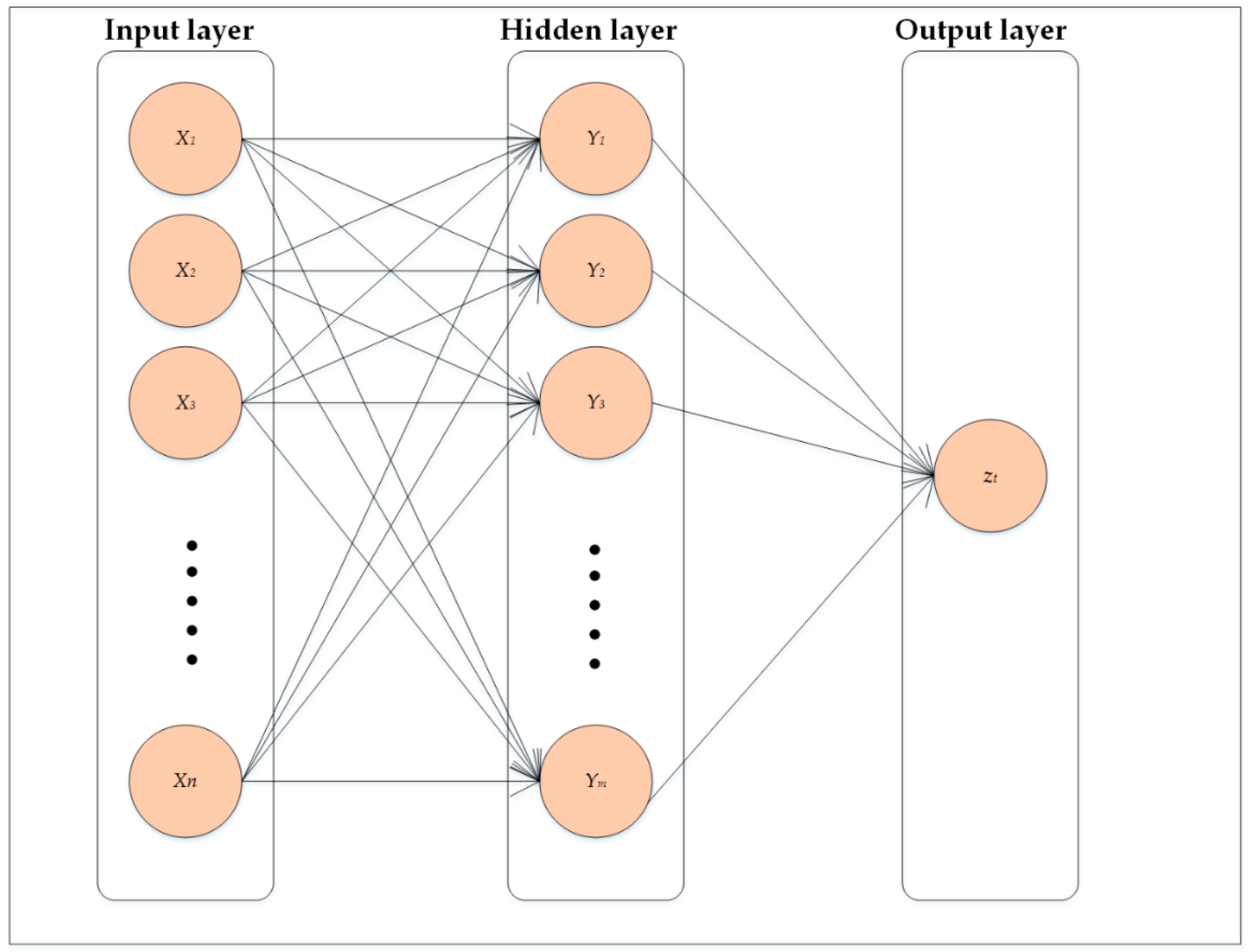
2.1. Artificial Neural Networks
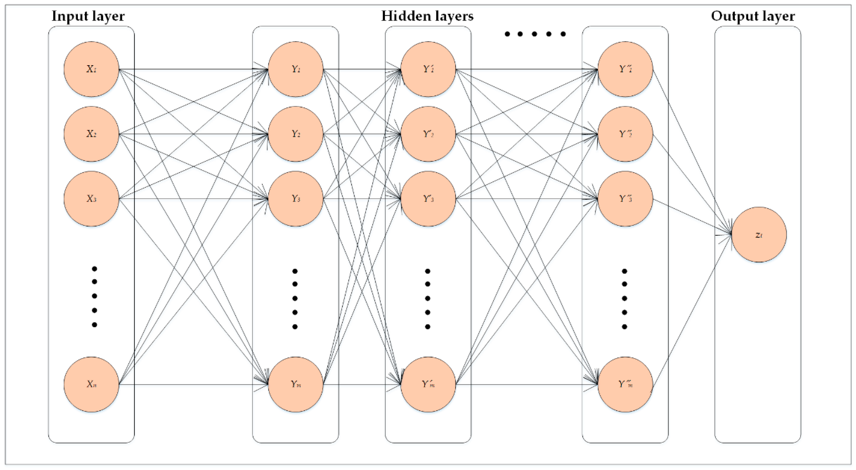
2.2. Deep Learning
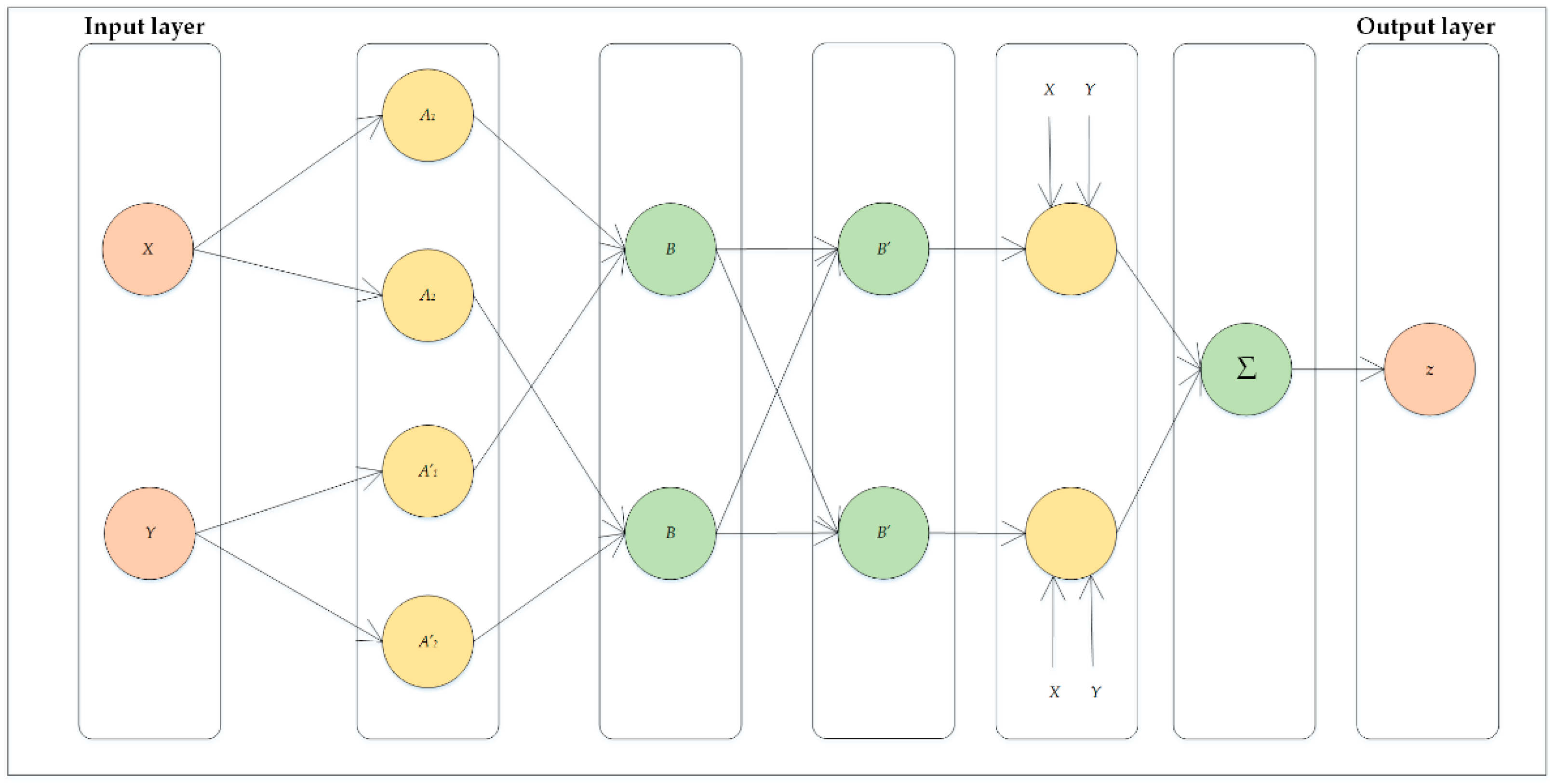
2.3. Kernel Models
2.4. Hybrid Models
3. Input Dataset
4. Conclusions and Future Outlook
Author Contributions
Funding
Institutional Review Board Statement
Informed Consent Statement
Data Availability Statement
Conflicts of Interest
Abbreviations
| AAPRE | Average Absolute Percent Relative Error |
| ACO | Ant Colony Optimization |
| AI | Artificial Intelligence |
| AIC | Akaike Information Criterion |
| ANFIS | Adaptive Neuro-Fuzzy Inference System |
| ANN | Artificial Neural Network |
| APE | Absolute Percentage Error |
| ARMA | Auto-Regressive Moving Average |
| BiLSTM | Bi-directional LSTM |
| BPNN | Backpropagation neural network |
| BT-GPR | Bayesian Tuned Gaussian Process Regression |
| BT-SVR | Bayesian Tuned Support Vector Regression |
| CANFIS | Co-Active Neuro-Fuzzy Inference System |
| CIT | Conditional Inference Tree |
| CNN | Convolutional Neural Network |
| ConvLSTM | Convolutional LSTM |
| CRM | Coefficient of Residual Mass |
| CRT | Classification and Regression Tree |
| DA | Dragonfly Algorithm |
| DL | Deep Learning |
| DNN | Deep Neural Network |
| DT | Decision Tree |
| EEMD | Ensemble Empirical Mode Decomposition |
| EEMD-Conv2d | Ensemble Empirical Mode Decomposition- Convolutional 2 dimension |
| EEMD-Conv3d | Ensemble Empirical Mode Decomposition- Convolutional 3 dimension |
| ELM | Extreme Learning Machine |
| ENN | Elman Neural Network |
| ERM | Empirical Risk Minimization |
| FARIMA | Fractionally Autoregressive Integrated Moving Average |
| FFA | FireFly Algorithm |
| FFBPNN | Feed Forward Back Propagation Neural Network |
| FFNN | Feed-Forward Neural Network |
| GA | Genetic Algorithm |
| GaP | Gaussian Process |
| GEP | Gene Expression Programming |
| GMDH | Group Method of Data Handling |
| GOA | Grasshopper Optimization Algorithm |
| GP | Genetic Programming |
| GRNN | Generalized Regression Neural Network |
| GRU | Gated Recurrent Unit |
| GSA | Gravitational Search Algorithm |
| GT | Gamma Test |
| GWO | Grey Wolf Optimizer |
| ICR | Independent Component Regression |
| IHR | Himalayan Region |
| KGE | Kling-Gupta Efficiency |
| KHA | Krill Herd Algorithm |
| k-NN | k-Nearest Neighbors |
| LAR | Least Angle Regression |
| LDAS | Land Data Assimilation System |
| LMI | Legates and McCabe Index |
| LR | Linear Regression |
| LSM | Land Surface Model |
| LST | Land Surface Temperature |
| LSTM | Long Short-Term Memory network |
| MABE | Mean Absolute Bias Error |
| MAPE | Mean Absolute Percentage Error |
| MARS | Multivariate Adaptive Regression Spline |
| MaxE | Maximum residual Error |
| MBE | Mean Bias Error |
| MLP | Multilayer Perceptron |
| MLR | Multiple Linear Regression |
| MSE | Mean Squared Error |
| mSG | A hybrid SSA-GOA algorithm including a mutation phase |
| M5 Tree | M5 Model Tree |
| NCPQR | Non Convex Penalized Quantile Regression |
| NDBaI | Normalized Difference Bareness Index |
| NDBI | Normalized Difference Built-up Index |
| NDVI | Normalized Difference Vegetation Index |
| NDWI | Normalized Difference Water Index |
| NLR | Non-Linear Regression |
| NN | Neural Network |
| NNLS | Non Negative Least Square |
| NRMSE | Normalized RMSE |
| NSE | Nash–Sutcliffe Efficiency |
| PBIAS | Percent Bias |
| PCA | Principal Component Analysis |
| PF | Persistence Forecast |
| PPR | Projection Pursuit Regression |
| PSO | Particle Swarm Optimization |
| RBNN | Radial Basis Neural Network |
| ResNet | Residual Network |
| RF | Random Forest |
| RMSE | Root Mean Square Error |
| RMSRE | Root Mean Squared Relative Error |
| RNN | Recurrent Neural Networks |
| RRMSE | Relative RMSE |
| SaE-ELM | Self-Adaptive Evolutionary ELM |
| SARIMA | Seasonal Auto-Regressive Integrated Moving Average |
| SFO | Sunflower Optimization |
| SHO | Spotted Hyena Optimizer |
| SI | Scatter Index |
| SMA | Slime Mold Algorithm |
| SMO | Sequential Minimal Optimization |
| SRM | Structural Risk Minimization |
| SSA | Salp Swarm Algorithm |
| STD | Standard Deviation |
| SVAT | Soil Vegetation Atmosphere Transfer |
| SVM | Support Vector Machine |
| SVR | Support Vector Regression |
| UI | Urban Index |
| VAF | Variance Accounted For |
| VRR | Variable Ridge Regression |
| WCANFIS | Wavelet transformation combined with CANFIS |
| WI | Willmott Index of Agreement |
| WNN | Wavelet Neural Network |
| WR2 | Weighted Coefficient of Determination |
| XGBoost | Extreme Gradient Boosting System |
References
- Verma, P.; Yeates, J.; Daly, E. A stochastic model describing the impact of daily rainfall depth distribution on the soil water balance. Adv. Water Resour. 2011, 34, 1039–1048. [Google Scholar] [CrossRef]
- Ali, I.; Greifeneder, F.; Stamenkovic, J.; Neumann, M.; Notarnicola, C. Review of machine learning approaches for biomass and soil moisture retrievals from remote sensing data. Remote Sens. 2015, 7, 16398–16421. [Google Scholar] [CrossRef]
- Colombo, R.; Bellingeri, D.; Fasolini, D.; Marino, C.M. Retrieval of leaf area index in different vegetation types using high resolution satellite data. Remote Sens. Environ. 2003, 86, 120–131. [Google Scholar] [CrossRef]
- Meroni, M.; Colombo, R.; Panigada, C. Inversion of a radiative transfer model with hyperspectral observations for LAI mapping in poplar plantations. Remote Sens. Environ. 2004, 92, 195–206. [Google Scholar] [CrossRef]
- Zhang, D.; Zhou, G. Estimation of soil moisture from optical and thermal remote sensing: A review. Sensors 2016, 16, 1308. [Google Scholar] [CrossRef] [PubMed]
- Monsivais-Huertero, A.; Graham, W.D.; Judge, J.; Agrawal, D. Effect of simultaneous state–parameter estimation and forcing uncertainties on root-zone soil moisture for dynamic vegetation using EnKF. Adv. Water Resour. 2010, 33, 468–484. [Google Scholar] [CrossRef]
- Khanal, S.; Fulton, J.; Shearer, S. An overview of current and potential applications of thermal remote sensing in precision agriculture. Comput. Electron. Agric. 2017, 139, 22–32. [Google Scholar] [CrossRef]
- Lakhankar, T.; Jones, A.S.; Combs, C.L.; Sengupta, M.; Vonder Haar, T.H.; Khanbilvardi, R. Analysis of large scale spatial variability of soil moisture using a geostatistical method. Sensors 2010, 10, 913–932. [Google Scholar] [CrossRef]
- Ghedira, H.; Lakhankar, T.; Jahan, N.; Khanbilvardi, R. Combination of passive and active microwave data for soil moisture estimates. In Proceedings of the IGARSS 2004. 2004 IEEE International Geoscience and Remote Sensing Symposium, Anchorage, AK, USA, 20–24 September 2004; IEEE: Piscataway, NJ, USA, 2004. [Google Scholar]
- Li, P.; Zha, Y.; Shi, L.; Tso, C.-H.M.; Zhang, Y.; Zeng, W. Comparison of the use of a physical-based model with data assimilation and machine learning methods for simulating soil water dynamics. J. Hydrol. 2020, 584, 124692. [Google Scholar] [CrossRef]
- Breen, K.H.; James, S.C.; White, J.D.; Allen, P.M.; Arnold, J.G. A hybrid artificial neural network to estimate soil moisture using swat+ and SMAP data. Mach. Learn. Knowl. Extr. 2020, 2, 16. [Google Scholar] [CrossRef]
- Karpatne, A.; Watkins, W.; Read, J.; Kumar, V. Physics-guided neural networks (pgnn): An application in lake temperature modeling. arXiv 2017, arXiv:1710.11431. [Google Scholar]
- Bergen, K.J.; Johnson, P.A.; de Hoop, M.V.; Beroza, G.C. Machine learning for data-driven discovery in solid Earth geoscience. Science 2019, 363, eaau0323. [Google Scholar] [CrossRef]
- Noé, F.; Olsson, S.; Köhler, J.; Wu, H. Boltzmann generators: Sampling equilibrium states of many-body systems with deep learning. Science 2019, 365, eaaw1147. [Google Scholar] [CrossRef] [PubMed]
- Hassan-Esfahani, L.; Torres-Rua, A.; Jensen, A.; McKee, M. Assessment of surface soil moisture using high-resolution multi-spectral imagery and artificial neural networks. Remote Sens. 2015, 7, 2627–2646. [Google Scholar] [CrossRef]
- Jiang, H.; Cotton, W.R. Soil moisture estimation using an artificial neural network: A feasibility study. Can. J. Remote Sens. 2004, 30, 827–839. [Google Scholar] [CrossRef]
- George, R.K. Prediction of soil temperature by using artificial neural networks algorithms. Nonlinear Anal. Theory Methods Appl. 2001, 47, 1737–1748. [Google Scholar] [CrossRef]
- Basheer, I.A.; Hajmeer, M. Artificial neural networks: Fundamentals, computing, design, and application. J. Microbiol. Methods 2000, 43, 3–31. [Google Scholar] [CrossRef]
- Nugroho, A.S. Information Analysis Using Softcomputing: The Applications to Character Recognition, Meteorological Prediction, and Bioinformatics Problems. Ph.D. Thesis, Nagoya Institute of Technology, Nagoya, Japan, 2003. [Google Scholar]
- Kisi, O.; Tombul, M.; Kermani, M.Z. Modeling soil temperatures at different depths by using three different neural computing techniques. Theor. Appl. Climatol. 2015, 121, 377–387. [Google Scholar] [CrossRef]
- Sanikhani, H.; Deo, R.C.; Yaseen, Z.M.; Eray, O.; Kisi, O. Non-tuned data intelligent model for soil temperature estimation: A new approach. Geoderma 2018, 330, 52–64. [Google Scholar] [CrossRef]
- Mehdizadeh, S.; Behmanesh, J.; Khalili, K. Evaluating the performance of artificial intelligence methods for estimation of monthly mean soil temperature without using meteorological data. Environ. Earth Sci. 2017, 76, 325. [Google Scholar] [CrossRef]
- Wu, W.; Tang, X.-P.; Guo, N.-J.; Yang, C.; Liu, H.-B.; Shang, Y.-F. Spatiotemporal modeling of monthly soil temperature using artificial neural networks. Theor. Appl. Climatol. 2013, 113, 481–494. [Google Scholar] [CrossRef]
- Ikechukwu, M.; Ebinne, E.; Yun, Z.; Patrick, B. Prediction of Land Surface Temperature (LST) Changes within Ikon City in Nigeria Using Artificial Neural Network (ANN). Int. J. Remote Sens. Appl. 2016, 6, 96–107. [Google Scholar]
- Araghi, A.; Mousavi-Baygi, M.; Adamowski, J.; Martinez, C.; van der Ploeg, M. Forecasting soil temperature based on surface air temperature using a wavelet artificial neural network. Meteorol. Appl. 2017, 24, 603–611. [Google Scholar] [CrossRef]
- Feng, Y.; Cui, N.; Hao, W.; Gao, L.; Gong, D. Estimation of soil temperature from meteorological data using different machine learning models. Geoderma 2019, 338, 67–77. [Google Scholar] [CrossRef]
- Sihag, P.; Esmaeilbeiki, F.; Singh, B.; Pandhiani, S.M. Model-based soil temperature estimation using climatic parameters: The case of Azerbaijan Province, Iran. Geol. Ecol. Landsc. 2020, 4, 203–215. [Google Scholar] [CrossRef]
- Tabari, H.; Sabziparvar, A.-A.; Ahmadi, M. Comparison of artificial neural network and multivariate linear regression methods for estimation of daily soil temperature in an arid region. Meteorol. Atmos. Phys. 2011, 110, 135–142. [Google Scholar] [CrossRef]
- Kim, S.; Singh, V.P. Modeling daily soil temperature using data-driven models and spatial distribution. Theor. Appl. Climatol. 2014, 118, 465–479. [Google Scholar] [CrossRef]
- Behmanesh, J.; Mehdizadeh, S. Estimation of soil temperature using gene expression programming and artificial neural networks in a semiarid region. Environ. Earth Sci. 2017, 76, 76. [Google Scholar] [CrossRef]
- Samadianfard, S.; Asadi, E.; Jarhan, S.; Kazemi, H.; Kheshtgar, S.; Kisi, O.; Sajjadi, S.; Manaf, A.A. Wavelet neural networks and gene expression programming models to predict short-term soil temperature at different depths. Soil Tillage Res. 2018, 175, 37–50. [Google Scholar] [CrossRef]
- Kaur, S.; Randhawa, S. Global land temperature prediction by machine learning combo approach. In Proceedings of the 2018 9th International Conference on Computing, Communication and Networking Technologies (ICCCNT), Bengaluru, India, 10–12 July 2018; IEEE: Piscataway, NJ, USA, 2018. [Google Scholar]
- Zare Abyaneh, H.; Bayat Varkeshi, M.; Golmohammadi, G.; Mohammadi, K. Soil temperature estimation using an artificial neural network and co-active neuro-fuzzy inference system in two different climates. Arab. J. Geosci. 2016, 9, 377. [Google Scholar] [CrossRef]
- Alizamir, M.; Kisi, O.; Ahmed, A.N.; Mert, C.; Fai, C.M.; Kim, S.; Kim, N.W.; El-Shafie, A. Advanced machine learning model for better prediction accuracy of soil temperature at different depths. PLoS ONE 2020, 15, e0231055. [Google Scholar] [CrossRef]
- Bilgili, M. Prediction of soil temperature using regression and artificial neural network models. Meteorol. Atmos. Phys. 2010, 110, 59–70. [Google Scholar] [CrossRef]
- Citakoglu, H. Comparison of artificial intelligence techniques for prediction of soil temperatures in Turkey. Theor. Appl. Climatol. 2017, 130, 545–556. [Google Scholar] [CrossRef]
- Ozturk, M.; Salman, O.; Koc, M. Artificial neural network model for estimating the soil temperature. Can. J. Soil Sci. 2011, 91, 551–562. [Google Scholar] [CrossRef]
- Shamshirband, S.; Esmaeilbeiki, F.; Zarehaghi, D.; Neyshabouri, M.; Samadianfard, S.; Ghorbani, M.A.; Mosavi, A.; Nabipour, N.; Chau, K.-W. Comparative analysis of hybrid models of firefly optimization algorithm with support vector machines and multilayer perceptron for predicting soil temperature at different depths. Eng. Appl. Comput. Fluid Mech. 2020, 14, 939–953. [Google Scholar] [CrossRef]
- Zeynoddin, M.; Ebtehaj, I.; Bonakdari, H. Development of a linear based stochastic model for daily soil temperature prediction: One step forward to sustainable agriculture. Comput. Electron. Agric. 2020, 176, 105636. [Google Scholar] [CrossRef]
- Seifi, A.; Ehteram, M.; Nayebloei, F.; Soroush, F.; Gharabaghi, B.; Torabi Haghighi, A. GLUE uncertainty analysis of hybrid models for predicting hourly soil temperature and application wavelet coherence analysis for correlation with meteorological variables. Soft Comput. 2021, 25, 10723–10748. [Google Scholar] [CrossRef]
- Paloscia, S.; Pampaloni, P.; Pettinato, S.; Santi, E. A comparison of algorithms for retrieving soil moisture from ENVISAT/ASAR images. IEEE Trans. Geosci. Remote Sens. 2008, 46, 3274–3284. [Google Scholar] [CrossRef]
- Hinton, G.E.; Osindero, S.; Teh, Y.-W. A fast learning algorithm for deep belief nets. Neural Comput. 2006, 18, 1527–1554. [Google Scholar] [CrossRef]
- Liu, Y.; Mei, L.; Ooi, S.K. Prediction of soil moisture based on extreme learning machine for an apple orchard. In Proceedings of the 2014 IEEE 3rd International Conference on Cloud Computing and Intelligence Systems, Shenzhen, China, 27–29 November 2014; IEEE: Piscataway, NJ, USA, 2014. [Google Scholar]
- LeCun, Y.; Bengio, Y. Convolutional networks for images, speech, and time series. Handb. Brain Theory Neural Netw. 1995, 3361, 1995. [Google Scholar]
- Hochreiter, S.; Schmidhuber, J. Long short-term memory. Neural Comput. 1997, 9, 1735–1780. [Google Scholar] [CrossRef] [PubMed]
- Shi, X.; Chen, Z.; Wang, H.; Yeung, D.-Y.; Wong, W.-K.; Woo, W.-C. Convolutional LSTM network: A machine learning approach for precipitation nowcasting. Adv. Neural Inf. Process. Syst. 2015, 28, 802–810. [Google Scholar]
- He, K.; Zhang, X.; Ren, S.; Sun, J. Deep residual learning for image recognition. In Proceedings of the IEEE Conference on Computer Vision and Pattern Recognition, Las Vegas Valley, NV, USA, 26 June–1 July 2016; IEEE: Piscataway, NJ, USA, 2016. [Google Scholar]
- Hao, H.; Yu, F.; Li, Q. Soil temperature prediction using convolutional neural network based on ensemble empirical mode decomposition. IEEE Access 2020, 9, 4084–4096. [Google Scholar] [CrossRef]
- Yu, F.; Hao, H.; Li, Q. An Ensemble 3D convolutional neural network for spatiotemporal soil temperature forecasting. Sustainability 2021, 13, 9174. [Google Scholar] [CrossRef]
- Imanian, H.; Hiedra Cobo, J.; Payeur, P.; Shirkhani, H.; Mohammadian, A. A Comprehensive Study of Artificial Intelligence Applications for Soil Temperature Prediction in Ordinary Climate Conditions and Extremely Hot Events. Sustainability 2022, 14, 8065. [Google Scholar] [CrossRef]
- Li, C.; Zhang, Y.; Ren, X. Modeling hourly soil temperature using deep BiLSTM neural network. Algorithms 2020, 13, 173. [Google Scholar] [CrossRef]
- Wang, X.; Li, W.; Li, Q. A new embedded estimation model for soil temperature prediction. Sci. Program. 2021, 2021, 5881018. [Google Scholar] [CrossRef]
- Imanian, H.; Shirkhani, H.; Mohammadian, A.; Hiedra Cobo, J.; Payeur, P. Spatial Interpolation of Soil Temperature and Water Content in the Land-Water Interface Using Artificial Intelligence. Water 2023, 15, 473. [Google Scholar] [CrossRef]
- Vapnik, V. The Nature of Statistical Learning Theory; Springer Science & Business Media: Berlin/Heidelberg, Germany, 1999. [Google Scholar]
- Pasolli, L.; Notarnicola, C.; Bruzzone, L. Estimating soil moisture with the support vector regression technique. IEEE Geosci. Remote Sens. Lett. 2011, 8, 1080–1084. [Google Scholar] [CrossRef]
- Adeyemi, O.; Grove, I.; Peets, S.; Domun, Y.; Norton, T. Dynamic neural network modelling of soil moisture content for predictive irrigation scheduling. Sensors 2018, 18, 3408. [Google Scholar] [CrossRef]
- Xing, L.; Li, L.; Gong, J.; Ren, C.; Liu, J.; Chen, H. Daily soil temperatures predictions for various climates in United States using data-driven model. Energy 2018, 160, 430–440. [Google Scholar] [CrossRef]
- Nanda, A.; Sen, S.; Sharma, A.N.; Sudheer, K. Soil temperature dynamics at hillslope scale—Field observation and machine learning-based approach. Water 2020, 12, 713. [Google Scholar] [CrossRef]
- Hong, Z. A Data-Driven Approach to Soil Moisture Collection and Prediction Using a Wireless Sensor Network and Machine Learning Techniques. Master’s Thesis, University of Illinois at Urbana-Champaign, Urbana Champaign, IL, USA, 2015. [Google Scholar]
- Okujeni, A.; Van der Linden, S.; Jakimow, B.; Rabe, A.; Verrelst, J.; Hostert, P. A comparison of advanced regression algorithms for quantifying urban land cover. Remote Sens. 2014, 6, 6324–6346. [Google Scholar] [CrossRef]
- Delbari, M.; Sharifazari, S.; Mohammadi, E. Modeling daily soil temperature over diverse climate conditions in Iran—A comparison of multiple linear regression and support vector regression techniques. Theor. Appl. Climatol. 2019, 135, 991–1001. [Google Scholar] [CrossRef]
- Moazenzadeh, R.; Mohammadi, B. Assessment of bio-inspired metaheuristic optimisation algorithms for estimating soil temperature. Geoderma 2019, 353, 152–171. [Google Scholar] [CrossRef]
- Guleryuz, D. Estimation of soil temperatures with machine learning algorithms—Giresun and Bayburt stations in Turkey. Theor. Appl. Climatol. 2022, 147, 109–125. [Google Scholar] [CrossRef]
- Penghui, L.; Ewees, A.A.; Beyaztas, B.H.; Qi, C.; Salih, S.Q.; Al-Ansari, N.; Bhagat, S.K.; Yaseen, Z.M.; Singh, V.P. Metaheuristic optimization algorithms hybridized with artificial intelligence model for soil temperature prediction: Novel model. IEEE Access 2020, 8, 51884–51904. [Google Scholar] [CrossRef]
- Bonakdari, H.; Moeeni, H.; Ebtehaj, I.; Zeynoddin, M.; Mahoammadian, A.; Gharabaghi, B. New insights into soil temperature time series modeling: Linear or nonlinear? Theor. Appl. Climatol. 2019, 135, 1157–1177. [Google Scholar] [CrossRef]
- Mustafa, E.K.; Co, Y.; Liu, G.; Kaloop, M.R.; Beshr, A.A.; Zarzoura, F.; Sadek, M. Study for predicting land surface temperature (LST) using landsat data: A comparison of four algorithms. Adv. Civ. Eng. 2020, 2020, 1–16. [Google Scholar] [CrossRef]
- Mehdizadeh, S.; Ahmadi, F.; Kozekalani Sales, A. Modelling daily soil temperature at different depths via the classical and hybrid models. Meteorol. Appl. 2020, 27, e1941. [Google Scholar] [CrossRef]
- Kisi, O.; Sanikhani, H.; Cobaner, M. Soil temperature modeling at different depths using neuro-fuzzy, neural network, and genetic programming techniques. Theor. Appl. Climatol. 2017, 129, 833–848. [Google Scholar] [CrossRef]
- Bayatvarkeshi, M.; Bhagat, S.K.; Mohammadi, K.; Kisi, O.; Farahani, M.; Hasani, A.; Deo, R.; Yaseen, Z.M. Modeling soil temperature using air temperature features in diverse climatic conditions with complementary machine learning models. Comput. Electron. Agric. 2021, 185, 106158. [Google Scholar] [CrossRef]
- Fathololoumi, S.; Vaezi, A.; Alavipanah, S.; Montzka, C.; Ghorbani, A.; Biswas, A. Soil temperature modeling using machine learning techniques. Desert (2008–0875) 2020, 25, 185–199. [Google Scholar]
- Mehdizadeh, S.; Fathian, F.; Safari, M.J.S.; Khosravi, A. Developing novel hybrid models for estimation of daily soil temperature at various depths. Soil Tillage Res. 2020, 197, 104513. [Google Scholar] [CrossRef]
- Malik, A.; Tikhamarine, Y.; Sihag, P.; Shahid, S.; Jamei, M.; Karbasi, M. Predicting daily soil temperature at multiple depths using hybrid machine learning models for a semi-arid region in Punjab, India. Environ. Sci. Pollut. Res. 2022, 29, 71270–71289. [Google Scholar] [CrossRef] [PubMed]
- Nahvi, B.; Habibi, J.; Mohammadi, K.; Shamshirband, S.; Al Razgan, O.S. Using self-adaptive evolutionary algorithm to improve the performance of an extreme learning machine for estimating soil temperature. Comput. Electron. Agric. 2016, 124, 150–160. [Google Scholar] [CrossRef]
- Samadianfard, S.; Ghorbani, M.A.; Mohammadi, B. Forecasting soil temperature at multiple-depth with a hybrid artificial neural network model coupled-hybrid firefly optimizer algorithm. Inf. Process. Agric. 2018, 5, 465–476. [Google Scholar] [CrossRef]
- Mehdizadeh, S.; Mohammadi, B.; Pham, Q.B.; Khoi, D.N.; Linh, N.T.T. Implementing novel hybrid models to improve indirect measurement of the daily soil temperature: Elman neural network coupled with gravitational search algorithm and ant colony optimization. Measurement 2020, 165, 108127. [Google Scholar] [CrossRef]
- Gill, J.; Singh, S. An efficient neural networks based genetic algorithm model for soil temperature prediction. Int. J. Emerg. Technol. Eng. Res. (IJETER) 2015, 3, 1–5. [Google Scholar]
- Le, V.T.; Quan, N.H.; Loc, H.H.; Duyen, N.T.T.; Dung, T.D.; Nguyen, H.D.; Do, Q.H. A multidisciplinary approach for evaluating spatial and temporal variations in water quality. Water 2019, 11, 853. [Google Scholar] [CrossRef]
- Almomani, A.; Wan, T.; Manasrah, A.; Altaher, A.; Almomani, E. A survey of learning based techniques of phishing email filtering. Int. J. Digit. Content Technol. Its Appl. 2012, 6, 119. [Google Scholar]


| Research | Models | Output | Input | Soil Depth | Performance Criteria | Best Model(s) |
|---|---|---|---|---|---|---|
| [20] | MLP, GRNN, RBNN, MLR | Monthly soil temperature | Relative humidity, solar radiation, wind speed, air temperature, soil temperature | 5, 10, 50, 100 cm | RMSE, MAE, R2 | RBNN at depths of 5 and 10 cm, MLR at depth of 50 cm, GRNN at depth of 100 cm |
| [21] | ANN, ELM, M5 Tree | Monthly soil temperature | Air temperature, relative humidity, wind speed, solar radiation, periodicity | 5, 50, 100 cm | R, RMSE, MAE, WI, NSE, LMI | ELM |
| [22] | ANN, ANFIS, GEP | Monthly soil temperature | Latitude, longitude, altitude, number of months | 5, 10, 50, 100 cm | R2, RMSE, MAE | ANFIS |
| [23] | ANN | Monthly soil temperature | Latitude, longitude, elevation, topographic wetness index, NDVI | 10 cm | RMSE, MAPE, R2 | |
| [24] | FFBPNN | Land surface temperature at 14 years’ interval | A sequence of past LST values, latitude, longitude | - | R, MSE | |
| [25] | ANN, WNN | Next 1 to 7 day soil temperature | Surface air temperature | 5, 10, 20, 30 cm | RMSE | WNN |
| [26] | ELM, GRNN, BPNN, RF | Half-hourly soil temperature | Air temperature, wind speed, relative humidity, solar radiation, and vapor pressure deficit | 2, 5, 10, 20 cm | RMSE, MAE, NSE, R | ELM |
| [27] | MLP, RF, GP, M5P | Daily soil temperature | Sunshine hours, wind speed, relative humidity, air temperature | 5 cm | MAE, RMSE, R | MLP |
| [28] | MLP, MLR | Daily soil temperature | Air temperature, solar radiation, relative humidity, precipitation | 5, 10, 20, 30, 50, 100 cm | R, RMSE, MAE | MLP |
| [29] | MLP, ANFIS | Daily soil temperature | Air temperature, relative humidity, dew point temperature, potential evapotranspiration, wind speed, solar radiation, soil temperature | 10, 20 cm | NSE, RMSE, MAE, APE | MLP |
| [30] | GEP, ANN, MLR | Daily soil temperature | Relative humidity, wind speed, extraterrestrial radiation, sunshine hours, minimum and maximum air temperature | 5, 10, 20, 30, 50, 100 cm | R2, RMSE | ANN |
| [31] | ANN, WNN, GEP | Daily soil temperature | Air temperature, solar radiation, pressure, soil depth, periodicity | 10, 20, 30, 50, 100 cm | R, MAE, RMSE, AIC, Taylor diagrams | WNN |
| [32] | An ensemble approach based on ANN, MARS, CIT, DT, ICR, k-NN, LAR, NNLS, NCPQR, PCA, Lasso, VRR, PPR | Land Surface Temperature | Latitude, longitude, temperature | Total computation time, RMSE, R2 | Model built by DT, VRR, and CIT. | |
| [33] | ANN, CANFIS | Daily soil temperature | Air temperature | 5, 10, 20, 30, 50, 100 cm | RMSE, R | ANN |
| [34] | ELM, ANN, CRT, GMDH | Monthly soil temperature | Air temperature, relative humidity, solar radiation, wind speed | 5, 10, 50, 100 cm | RMSE, R2 | ELM |
| [35] | FFBPNN, LR, NLR | Monthly soil temperature | Air temperature, atmospheric pressure, solar radiation, depth, month | 5, 10, 20, 50, 100 cm | MAPE, R | FFBPNN |
| [36] | ANN, ANFIS, MLR | Monthly soil temperature | Minimum and maximum air temperature, calendar month number, depth of soil, precipitation | 5, 10, 20, 50, 100 cm | RMSE, MAE, R2 | ANFIS |
| [37] | FFNN | Monthly mean soil temperature | Altitude, latitude, longitude, month, year, solar radiation, sunshine duration, air temperature | 5, 10, 20, 50, 100 cm | RMSE, R | |
| [38] | SVM, MLP, SVM-FFA, MLP-FFA | Soil temperature | air temperature, relative humidity, sunshine hours, wind speed | 5, 10, 20 cm | RMSE, MAE, R | MLP-FFA |
| [39] | SARIMA, ELM, SaE-ELM, ANFIS | Daily soil temperature | Soil temperature | 5, 10, 20, 30, 50, 100 cm | RMSE, MAPE, R2 | SARIMA |
| [40] | ANFIS, SVM, RBNN, MLP optimized by the FFA, SFO, SSA, and PSO algorithms | Hourly soil temperature | Air temperature, relative humidity, solar radiation, wind speed | 5, 10, 30 cm | NSE, RMSE, MAE, R2, PBIAS | ANFIS-SFO |
| Research | Models | Output | Input | Soil Depth | Performance Criteria | Best Model(s) |
|---|---|---|---|---|---|---|
| [48] | EEMD-CNN, PF, BPNN, LSTM, EEMD-LSTM | Next 1, 3, 5 day’s soil temperature | Soil temperature at different depths and areas | 5, 10, 30 cm | MSE, RMSE, MAE, R2 | EEMD-CNN, EEMD-LSTM |
| [49] | EEMD-Conv3d, Conv2D, Conv3D, ConvLSTM, EEMD-Conv2D, EEMD-ConvLSTM | Next 1, 3, 5 day’s soil temperature | Soil temperature | 7 cm | MSE, RMSE, MAE, R2, MAPE | EEMD-Conv3d |
| [50] | LR, ridge regression, Lasso, ENet, DT, RF, k-NN, XGBoost, SVM, gradient boosting, stacking methods, MLP, DL, ANFIS | Hourly soil temperature | Air temperature, precipitation, surface pressure, evaporation, wind speed, dew point temperature, solar radiation, thermal radiation | 7 cm | MAE, MSE, RMSE, R2, MAPE | DL, MLP, stacking model |
| [51] | BiLSTM, LSTM, DNN, RF, SVR, LR | Hourly soil temperature | Maximum and minimum air temperature, wind speed, solar radiation, maximum and minimum relative humidity, vapor pressure, dew point temperature | 5, 10, 20, 50, 100 cm | RMSE, MAE, R2 | BiLSTM |
| [52] | GRU-based model, ANN, ELM, LSTM | Soil temperature at different time points (6 h, 12 h, 24 h) | Historical soil temperature | 5, 10, 15 cm | RMSE, MAE, MSE, R2 | GRU-based model |
| [53] | RBFN, DL, spline deterministic spatial interpolation method | Soil temperature | Soil temperature, soil moisture, climate data | 10 cm | RMSE, NRMSE, SI, MAPE, Bias, R2, MAE, NSE, VAF, AIC, MSE, MaxE | DL |
| Research | Models | Output | Input | Soil Depth | Performance Criteria | Best Model(s) |
|---|---|---|---|---|---|---|
| [57] | SVM | Daily soil temperature | Humidity, wind speed, radiation, soil temperature, air temperature, time of year | 5, 10, 20, 50, 100 cm | RMSE, MAE, R2 | |
| [58] | XGBoost, SVM, RF, MLP | Hourly and half-hourly soil temperature | Rainfall, soil moisture, soil temperature, air temperature, relative humidity, vapor pressure deficit, solar radiation | 15 cm | R2, MAE | XGBoost |
| [61] | SVR, MLR | Daily soil temperature | Minimum and maximum air temperature, solar radiation, relative humidity, dew point temperature, atmospheric pressure | 10, 30, 100 cm | NRMSE, MBE, NSE, R2, WR2 | SVR |
| [62] | SVR, ENN, SVR-FFA, ENN-FFA, SVR-KHA, ENN-KHA | Daily soil temperature | Air temperature, sunshine hours, relative humidity, wind speed, pressure deficit | 5, 10, 20, 30, 50, 100 cm | RMSE, MARE, R2 | SVR-KHA |
| [63] | LSTM, BT-SVR, BT-GPR | Daily soil temperature | Cloudiness, air temperature, relative humidity, precipitation, pressure | 5, 10, 20, 50 cm | R2, RMSE, MAE | BT-GPR |
| Research | Models | Output | Input | Soil Depth | Performance Criteria | Best Model(s) |
|---|---|---|---|---|---|---|
| [64] | ANFIS, ANFIS-SSA, ANFIS-GOA, ANFIS-mSG, ANFIS-GWO, ANFIS-PSO, ANFIS-GA, ANFIS-DA | Daily soil temperature | maximum, average, and minimum air temperature | 10 cm | RMSE, STD, MAE, RMSRE, AAPRE, R2, NSE | ANFIS-mSG |
| [65] | MLP, ANFIS, MLP-PSO, ANFIS-PSO, ARMA | Daily soil temperature | Average, minimum, maximum, median, standard deviation, coefficient of variation, skewness, kurtosis, first quarter, and third quarter | 10, 20 cm | R2, MAE, RMSE, MAPE | ARMA |
| [66] | MARS, WNN, ANFIS, DENFIS | Land surface temperature | NDVI, NDBI, NDWI, NDBaI, UI, elevation | - | R2, RMSE, MAE | ANFIS |
| [67] | ANFIS, bi-linear model, hybrid models based on ANFIS, bi-linear, and wavelet analysis | Daily soil temperature | Soil temperature | 5, 10, 50, 100 cm | RMSE, MAE, KGE | ANFIS model combined with bi-linear and wavelet analysis |
| [68] | ANN, ANFIS, GP | Monthly soil temperature | Air temperature, relative humidity, solar radiation, wind speed, month of year, soil temperature at different depths | 10, 20, 100 cm | RMSE, MARE, R2, NSE | GP |
| [69] | ANN, CANFIS, WNN, WCANFIS | Soil temperature | Air temperature | 5,10,20,30, 100 cm | NSE, RMSE, CRM | WCANFIS |
| [70] | ANN, ANFIS, MLR | Air temperature, soil temperature, environmental parameters, soil properties | 5, 10 cm | R2, MAPE | ANFIS | |
| [71] | FARIMA, FFBPNN, GEP GEP-FARIMA, FFBPNN-FARIMA | Daily soil temperature | Historical records of soil temperature data | 5, 10, 50, 100 cm | RMSE, MAE, RRMSE | GEP-FARIMA |
| [72] | SVM, MLP, and ANFIS hybridized with SMA, PSO, and SHO | Daily soil temperature | Relative humidity, wind speed, solar radiation, air temperature | 5, 15, 30 cm | MAE, RMSE, IS, NSE, R, WIA, radar chart, scatter plots, box-whisker plot, Taylor diagram | SVM-SMA |
| [73] | ELM, SaE-ELM, ANN, GP | Daily soil temperature | Minimum, maximum, and average air temperature | 5, 10, 20, 30, 50, 100 cm | MAPE, RMSE, R | SaE-ELM |
| [74] | MLP, MLP-FFA | Monthly soil temperature | Soil depth, periodicity (or the respective month), air temperature, atmospheric pressure, solar radiation | 5,10,20,50, 100 cm | RMSE, MAE, MAPE, MBE, Taylor diagram | MLP-FFA |
| [75] | ENN-GSA, ENN-ACO | Daily soil temperature. | Mean temperature, maximum temperature, minimum temperature, dew point temperature, wind speed, relative humidity, precipitation, sunshine hours, soil temperature | 5, 10, 50, 100 cm | RMSE, RRMSE, R2, a-20 index | ENN-GSA |
| [76] | ANN- based model boosted by genetic algorithm | Daily soil temperature | Air temperature, rainfall, past soil temperature data | 5, 10, 30 cm | Error value |
| Model | Strength | Weakness |
|---|---|---|
| ANN |
|
|
| DL |
|
|
| Kernel-based |
|
|
| Hybrid |
|
|
Disclaimer/Publisher’s Note: The statements, opinions and data contained in all publications are solely those of the individual author(s) and contributor(s) and not of MDPI and/or the editor(s). MDPI and/or the editor(s) disclaim responsibility for any injury to people or property resulting from any ideas, methods, instructions or products referred to in the content. |
© 2023 by the authors. Licensee MDPI, Basel, Switzerland. This article is an open access article distributed under the terms and conditions of the Creative Commons Attribution (CC BY) license (https://creativecommons.org/licenses/by/4.0/).
Share and Cite
Taheri, M.; Schreiner, H.K.; Mohammadian, A.; Shirkhani, H.; Payeur, P.; Imanian, H.; Cobo, J.H. A Review of Machine Learning Approaches to Soil Temperature Estimation. Sustainability 2023, 15, 7677. https://doi.org/10.3390/su15097677
Taheri M, Schreiner HK, Mohammadian A, Shirkhani H, Payeur P, Imanian H, Cobo JH. A Review of Machine Learning Approaches to Soil Temperature Estimation. Sustainability. 2023; 15(9):7677. https://doi.org/10.3390/su15097677
Chicago/Turabian StyleTaheri, Mercedeh, Helene Katherine Schreiner, Abdolmajid Mohammadian, Hamidreza Shirkhani, Pierre Payeur, Hanifeh Imanian, and Juan Hiedra Cobo. 2023. "A Review of Machine Learning Approaches to Soil Temperature Estimation" Sustainability 15, no. 9: 7677. https://doi.org/10.3390/su15097677