Optimization of Green Containerized Grain Supply Chain Transportation Problem in Ukraine Considering Disruption Scenarios

Abstract

Grain supply chain transportation problem is a nontrivial and intractable issue for many developing countries. Grain as a bulk commodity is usually transported by bulk carriers. By taking into account the special condition of Ukraine, we proposed the containerized grain supply chain transportation optimization problem. In this problem, the sustainable supply chain system delivers grains in containers among primary elevators, intermodal yards, and port container terminals. Then, a containerized grain transportation model was developed to minimize the total cost of the sustainable supply chain system. Specifically, 20-foot containers were proven as more reasonable to be used in this paper. We also considered different transportation tools: trucks that can load one 20-foot container, trailers that can load two 20-foot containers, and wagons that can hold two 20-foot containers. Additionally, a disruption model was proposed by considering different disruption scenarios. Based on an analysis of the simulation results, some cost minimization strategies were proposed. Finally, a sensitivity analysis that aimed to analyze the effect of the proposed strategies on the minimal total cost and sustainability of the supply chain was conducted. The main conclusions drawn from the simulation are that the established food supply chain model is meaningful and accurate, and the incorporation of the disruption model aligns with practical requirements. Additionally, an increase in intermodal yard capacity, truck park size, and wagon park size decreases the total cost of the supply chain. The first two have a positive effect on the sustainability of the supply chain, while the latter increases the disruption risk of the supply chain.

1. Introduction

The crops grown on Ukrainian plains include wheat, barley, and sugar beets. Ukraine is also referred to as “the breadbasket of Europe”. However, according to the government report “Updated National Transport Strategy of Ukraine” (2016), logistics problems have always restricted the development of grain bulk transportation in Ukraine, including a lack of multimodal transport solutions benefiting long-distance haulage, and over-challenged capacities of seaports in handling bulk grains. Grain harvest is seasonal, so the demand for wagons is also seasonal, and so far, there are no other alternative methods for Ukrainian grain transportation other than replacing regular wagons with special wagons. This problem can be solved through the use of dry containers for grain delivery. Ukraine mainly imports high-value industrial products using containers and mainly exports raw materials using bulk carriers, which causes an imbalance in import and export containers. There are many empty containers transferred back to the place of departure in Ukraine; thus, we can consider the rational use of empty containers, which are relatively cheap and can be easily loaded onto wagons, trucks, and trailers. Additionally, an increase in the share of grain transported by containers will also ease the pressure on bulk grain processing at a port. It can also create more chances for transporting smaller quantities of higher-value grains. A previous study found that the speed of container systems and just-in-time scheduling reduced the risk of spoilage due to insects, pests, rancidity, discoloration, etc., and discussed potential effects on sustainability improvement [1]. Additionally, containerized grain transportation conforms to the trend of green grain logistics. Maiyar and Thakkar [2] developed a hub-and-spoke network based a multi-objective green transportation model for evaluating optimal shipment quantity, modal choice, route selection, hub location, and vehicle velocity decisions, considering wastages in the Indian food grain context. The traditional low-efficiency production-cost mode of bulk cargo transportation, the clean production mode of operation port, and environmental protection technology were gradually eliminated; this approach also responded to current development needs, mainly in reducing the labor intensity of workers, improving the working environment of workers, reducing carbon emissions, and reducing environmental damage, and, thus, the mode of transportation of “scattered change set” can be produced [3]. This paper suggests the use of dry vent containers as an alternative cargo handling and transportation unit for grain transportation to its final destination in Ukraine, which is sustainable for the environment.

This paper has a significant effect on the popularization of the idea of containerized grain transportation in Ukraine. It provides farmers and grain traders with information that describes the benefits of containerized grain transportation. Containerized grain transportation is also greener and more environmentally sustainable compared to traditional bulk cargo transportation. Again, this study seeks to provide insightful knowledge about disruption problems in supply chain activities, particularly in grain transportation, and suggests a mathematical model for resolving such disruption, which can be used as a reference for planning and scheduling of the grain-delivery supply chain in Ukraine.

The remainder of this paper is organized as follows. Section 2 reviews the relevant literature. Section 3 provides problem description and mathematical formulation. Section 4 describes the simulation of the models and provides some discussions. Finally, concluding remarks are discussed in Section 5.

2. Literature Review

We review the relevant literature, including grain supply chain storage and transportation problem and grain supply chain disruption management problem.

2.1. Grain Supply Chain Storage and Transportation Problem

The development of container transportation in the agriculture field will build up agricultural export potential in Ukraine [4]. Additionally, many studies have been conducted on the grain supply chain transportation problem. These studies have concentrated on the different aspects of the problem and suggested different approaches to it. Olexiy Pavlenko and Denis Velykodnyi [5] analyzed the technology used to transport grain cargoes in containers for international trade and identified three different options in Ukraine. The first option involves using rail transport (grain cars) to transport grain to the departure port. The second option involves using road transport (bulk grain lorries) to transport grain to the departure port. The third option involves using containers and carriages to transport grain to the departure port. Additionally, Kovalov et al. [6] discussed the option of using multiple grain shipping containers and introducing modern cargo handling technology at a station, which required efficient inventory management and vehicle selection. Ahumada and Villalobos [7] reviewed successfully implemented supply chain planning models for the production and distribution of agricultural products. The operational planning model for the production and distribution of perishable agricultural products was studied by Ahumada and Villalobos [8]. Asgari et al. [9] solved the wheat storage and transportation problem in Iran by creating a linear integer programming model and solving it with a genetic algorithm using the LINGO software. However, the authors did not include the operational cost, multimodal transportation, vehicle availability, and capacity constraints in their study. Agustina et al. [10] investigated cross-docking of a grain supply chain to deliver the commodity with the least total cost, in particular in holding and transportation costs. A cost-efficient model for Indian grain supply chain transportation with a consideration of multimodal transportation was developed by Maiyar et al. [11]. Inventory holding cost, vehicle capacity constraints, and allocation decisions were not covered by their study. Lamsal et al. [12] developed a mathematical model for harvest transportation from farms to customers by considering multiple independent farmers and no storage at the farms, and the authors considered multiple types of crops. Mogale et al. [13] studied a multi-period model for the Indian grain supply chain and tried to achieve optimal transportation, capacity, and allocation of silos. The following were the contributions of their paper: (1) taking into account seasonal procurement, inventory and operational costs of grain, fixed costs of capacitated silos, variety of vehicles parked, vehicle preference constraints, railroad flexibility, and a definite planning horizon, and (2) creating a variant of the Max–Min Ant System algorithm, named Improved Max–Min Ant System (IMMAS). It was used to solve the mixed-integer nonlinear programming model under time limitation. Gholamian and Taghanzadeh [14] investigated the multi-period problem of wheat supply chain in Iran to estimate the number and location of silos and the quantity of hold inventory at each location. The authors proposed an integer linear model to solve the problem and were able to achieve a significant reduction in transportation costs for the Iranian wheat supply chain. Mogale et al. [15] proposed a grain silo location-allocation problem with dwell time for the optimization of a food grain supply chain network. Additionally, two Pareto-based multi-objective algorithms with calibrated parameters were used to optimize two conflicting objectives: minimization of total grain supply chain network cost and total lead time (transit and dwell time).

2.2. Grain Supply Chain Disruption Management Problem

Disruption is a risk event that disturbs the internal processes of a supply chain network. Wagner and Bode [16] referred to disruptions as a combination of unexpected and abnormal events that appear in a supply chain or its surrounding environment, and this results in situations which significantly threaten the normal operations of the supply chain. Supply chain disruption may appear at any level due to factory closing, quarantines, accidents, etc. Additionally, Passarelli et al. [17] summed up various supply chain disruption challenges. Disruptions in supply chains may be considered from the perspective of three separate risk events, depending on the focus of how to manage the disruptive events: uncertainty, vulnerability, and crisis.

Uncertainties are events in a supply chain that are difficult to predict and forecast [18]. The likelihood or probability of an outcome that may occur in a supply chain can be used to recognize the causes of disruptive events in the supply chain. There are many pieces of research conducted on the topic of uncertainty in supply chain systems. For example, agricultural production planning under uncertainty in the Czech Republic was studied by Janová [19]. MIP has become a common tool for many scholars; for instance, Tsiakis et al. [20] used mixed-integer programming to simulate a multi-echelon supply chain under demand uncertainty.

Another way of discussing disruptions in terms of the level of consequences they have on the normal work of a supply chain is vulnerability [21]. A later study [22] investigated the impact of disruptions on inbound and outbound flows of an automotive assembler. Additionally, the probability of disruptions occurring from and through a supply chain is related to the complexity, severity, and density of the supply chain network. The higher the complexity of a supply chain network, the higher the probability.

The third way to discuss disruptions is through a crisis perspective. A disruption creates critical and chaotic conditions and results in a loss of the capabilities to provide services in a supply chain. However, Brockner and Erika [23] stated that this situation can be used by a supply chain entity to develop improved ways to provide services.

2.2.1. Disruption Management Process

There are two ways that researchers have approached the disruption problem: the first way is to approach it from the perspective of preparations [24], and the other is to approach it from the perspective of the response used in handling disruptions.

(1)

Mitigation approach

Disruption mitigation can be defined as risk preparation to avoid, and not simply respond to, disruptions that may impact the supply chain of a company [25]. There are many methods of mitigating risk that have been widely studied by many scholars: risk prevention, risk evaluation, risk assessment, risk policy, financial allocation, and monitoring and controlling.

(2)

Disruption management approach

The disruption management approach aims to alleviate the consequences of disruptions. However, from a time-based perspective, there are only a few concepts for managing transport disruptions: pre-disruption, during disruption, and post-disruption stages. The majority of papers on the topic of disruption management have focused on the combination of these three concepts.

2.2.2. Grain Supply Chain Disruption Problem

In recent years, many academic studies have been conducted on the topic of supply chain disruption because disruption at any stage of a supply chain can cause the entire system to fail. Most commonly, this kind of research has concentrated on the decision-making process in managing disruption risks [16]. Many studies have also been conducted on supply chain performance, taking the occurrence of supply disruptions into consideration, with some studies focusing on production [26], distribution [22], or the combination of production and distribution in a production–distribution system [18]. The role of transport operations is essential in solving the disruption problem because of the density and complexity of transportation linkages in a supply chain [27]. Many studies have been conducted on transportation disruptions in supply chains in the fields of pipelines [28], road transport [18], airline operations [29,30], and recovery of maritime transport [31]. These studies have mainly evaluated disruptions in a supply chain in terms of transportation performance and service unavailability in the supply chain. Relatively few studies have considered intermediate-node disruptions. Hatefi and Jolai [32] proposed a mixed-integer linear programming model with augmented $p$-robust constraints to control the reliability of a forward–reverse logistics network for solving disruption scenarios.

3. Problem Description and Mathematical Formulation

3.1. Problem Description

Every supply chain of containerized grains is expected to start at a farm. The cleaned or uncleaned grains that have been harvested on the farm are moved by trucks or tractors to the nearest primary elevator in bulk. At the primary elevator, grains go through sampling, cleaning, and weighting before storing. When the primary elevator receives an order, it loads grains into containers. At this stage, the decision of what size containers should be used is made, and this decision is based on the bulk density of each specific grain.

Table 1. Bulk density of grains.

Type of Grain	Barley	Corn	Oats	Rye	Wheat
Average value between different sources, kg/m3	619	720	447	719	757

presents the average bulk density for different types of grains that are commonly exported from Ukraine and provided by different sources and the average value between them.

Table 2. Weight of full load of grains.

Container Type	$\mathbf{Volume}, {\mathbf{m}}^3$	Gross Weight, kg	Tare Weight, kg	Payload, kg	Weight of Full Load of Barley, kg	Weight of Full Load of Corn, kg	Weight of Full Load of Oats, kg	Weight of Full Load of Rye, kg	Weight of Full Load of Wheat, kg
20 feet Standard dry	33.2	30,480	2200	28,280	20,550	23,904	14,840	23,870	25,132
40 feet Standard dry	67.3	32,500	3640	28,860	41,658	48,456	30,083	48,388	50,946

provides additional information about the most common container types’ volume, their gross capacity, the empty weight of these containers, and the weight of the full load of different types of grains. As we can see in Table 2, the payload of 20- and 40-foot containers are almost the same, and the weight of the full load of a 40-foot container for most types of grains greatly exceeds the payload of the container. This means that a 40-foot container only provides an additional couple of tons of carrying capability compared to a 20-foot container; however, a 40-foot container’s shipment, handling, and storage costs are significantly more expensive. That is why it is reasonable to advise the usage of 20-foot containers as being more economically feasible for the transportation of most common grains in Ukraine, with the exception of oats.

After the decision is made, containers are cleaned and dried, their rubber door seals are inspected, and disposable shields are installed to minimize the pressure on the doors. Then, the containers are loaded on a truck. In Ukraine, containers are most commonly loaded on trucks and trailers in the following combinations: one 40-foot container, one 20-foot container, or two 20-foot containers. The loaded truck then delivers the containers either to a port container terminal or to an intermodal yard that has a railroad connection. It should be mentioned that railroad transportation is only used if the distance from a primary elevator to a port is relatively long, which gives an opportunity to lower the transportation cost due to the use of the economy of scale. At the intermodal yard, the containers are unloaded from the trucks and stored until train arrival. When the number of containers to be delivered reaches 54 (the capacity of one locomotive), a locomotive pickup service is provided by Ukrainian railways. After the train arrives, the containers are loaded on the wagons. Typically, one wagon can hold either one 40-foot or two 20-foot containers. The next link in the international containerized grains supply chain is a port container terminal. At the port, the containers are unloaded from the wagons and stored until the scheduled container vessel arrival. The cargo ship then takes the grain containers to the port of destination. From there, containerized grains are delivered to the final customers, most commonly by trucks or railroad.

3.1.1. Transportation Problem

In Sweden, grain farmers and transporters are integrated into the Swedish Farmers Supply and Crop Marketing Association, and transporters all operate through a common interface created by the Swedish Farmers Supply and Crop Marketing Association called “Lantmännen Direkt”, which is basically a common user interface whereby grain farmers communicate with their transport operators [33]. In order to minimize the transportation cost of farmers, the system allows farmers to schedule for pickup by giving all material facts about a cargo, including when to pick up, the location of grain and destination, quantity, and all other needed information about the cargo. One of the objectives of this paper is to minimize the total cost of containerized grain shipment in a supply chain located in Ukraine. For ease of calculation, the modulated supply chain begins at the intake of the primary elevator and ends at the port container terminal. The primary elevator is an initial point for pricing, cleaning, weighing, sorting, and blending, and a checkpoint for disease and insect control. A second reason for using the primary elevator as a start point is that trucking costs vary on a farm-to-farm basis, depending upon distance, volume, truck or tractor configuration, and services used. However, most of the primary elevators in Ukraine do not have a railway connection; therefore, in order to take advantage of the low cost of railway transportation, containers should be sent to an intermodal yard first. Railway transportation has the advantage of a lower shipment cost for a large number of products to be delivered to destinations located far away. Trucks, on the other hand, perform better when the distance from the primary elevator to the port container terminal is relatively short. The port container terminal is chosen to be the endpoint of our system as it is the last supply chain point geographically located in Ukraine. The contracts that clients sign with cargo shipping companies will create the demand for our supply chain. This paper focuses on only three stages of the containerized grain supply chain, which include the delivery of containers from the primary elevator to the intermodal yard and from the intermodal yard to the port container terminal, with the possibility of direct delivery of containers from the primary elevator to the port container terminal. A depiction of the transportation problem is shown in Figure 1.

The proposed model is a multi-period model, so it minimizes the total cost of the supply chain through all time periods. In this model, we consider three months (one quarter) as the duration of each time period.

This model aims to minimize the total cost of transportation of containerized grains from the primary elevator to the port container terminal, including the transportation cost of road and rail transportation, inventory holding cost in bulk at the PE, inventory holding cost of containers at the IY, and operational cost at the PE, IY, and PCT. We consider containerized grain transportation, which is different from traditional bulk grain transportation in the aspects of grain handling, loading and unloading, storage, and transportation. In order to achieve a suitable result, a number of challenges should be overcome, such as truck selection problem and container selection problem.

The total transportation cost consists of fixed and variable transportation costs. Fixed transportation cost varies depending on the type of vehicle or wagon that is used. Variable transportation cost is influenced not only by the cost of transportation for different types of trucks and wagons (per unit per distance), distance and weight of grains, but also by the weight of the container itself.

At the PE, grains are stored in bulk and loaded into containers right before loading the containers into a truck. Therefore, the inventory holding cost should be calculated in bulk. On the other hand, the IY, after receiving containers, stores them until the scheduled train arrival, so the inventory holding cost of the IY should be calculated in a different manner. In this model, each time period is three-month long, and grain delivery can be received or shipped at any point of time throughout this time period; hence, the inventory holding cost is calculated as an arithmetic mean between the quantity of grain at the beginning and end of each period that is multiplied by the unit inventory holding cost per time period.

At the PE, a part of the operational cost occurs due to pricing, cleaning, weighting, sorting, blending, and quality control. This part of the operational cost occurs only once after grains are received by the PE from farms. Other sources of operational cost are the loading of bulk grains into containers (including container cleaning and drying cost, cost of final quality inspection of grains and containers, and cost of disposable shields) and loading of containers onto trucks. The only source of the operational costs at the IY and PCT are the loading and unloading of containers to and from trucks and wagons.

3.1.2. Disruption Management Problem

Any supply chain in the world has the chance of being disrupted by unexpected natural or man-made disasters. The probability of such disaster events is very low, but their business impact can be very high. COVID-19 has volatile, uncertain, complex, and ambiguous elements [34]. An example of such a disruption is the COVID-19 pandemic, which has greatly affected the global economy, and many companies all over the world have suffered from big financial losses, some of which even have to declare bankruptcy. The events of recent years have shown the importance of creating a supply chain that can minimize the impact of disruptions. Another objective of this paper is to minimize the expected total cost of the supply chain and to consider the possibility of disruption of IY operations in Ukraine. Such a disruption can be caused by natural disasters (earthquake, flood, hurricane, major snowfall, etc.), technological disaster (fire, explosion, etc.), failure of railroad or road system that linked to an IY, workers’ strike, etc. In the event of such disruption, an IY cannot fully fulfill its obligations, which can lead to delay or order cancellation. Given a set of customer orders for grain delivery to a specific PCT, a decision-maker needs to decide which PE or group of PEs to select to supply the grains required to complete customer orders and how to schedule the transportation of containerized grains over the planning horizon to mitigate the impact of disruption risks. In this paper, we consider the probability of all disruption scenarios. Each disruption scenario represents a unique subset of IYs that are currently disrupted or that are working without disruption at any given point of time. We consider that in case of a disruption, an IY will lose 50% of its capacity at a given period of time. This model considers multiple time periods that are three-month long. We assume that in case of a disruption in the previous time period, an IY will be able to recover its capacity in this time period since a time of three months is an adequate amount of time to solve most of the possible disruption causes. The modulated supply chain is organized in such a way that even with the disruption of all IYs, the delivery of grains is still possible due to direct truck delivery from the PE to the PCT, but at a greater cost. A depiction of the disruption management problem is shown in Figure 2. The red color in the figure indicates that the IYs have been interrupted.

3.2. Mathematical Formulation

3.2.1. Assumptions

The model is based on the following assumptions regarding containerized grain supply chain in Ukraine:

(1)

The procurement at primary elevators and the demand of each port are deterministic in nature and well known with little variation. This paper does not consider a stochastic environment. The contracts that are signed with shipment companies create the demand that are known and fixed; therefore, demand is taken as a deterministic parameter.

(2)

This model is based on the example of wheat transportation because wheat is the dominant export grain in Ukraine.

(3)

A finite number of capacitated trucks and wagons are available at each primary elevator and intermodal yard in each period. This paper considers the use of the most typical 20-foot containers. In this model, containers are loaded on trucks and trailers in two combinations: one 20-foot container or two 20-foot containers. One wagon can typically hold two 20-foot containers.

(4)

The variable shipment cost is related to the traveled distances among the supply chain nodes.

(5)

The procured grain quantity is enough to fulfill the demand of each port in each time period. This paper does not consider shortage, backlog, and penalty cost.

(6)

We consider 20-foot container size for storage and shipments of grains as being most suitable for grain transportation based on the bulk density. An infinite number of containers is available at each primary elevator in each period.

3.2.2. Mathematical Formulation of the Transportation Problem

The mathematical model for the containerized grain shipment and storage is shown below:

Minimize $z$ = Transportation cost $F_1$ + Operating cost $F_2$ + Inventory cost $F_3$

Transportation cost $F_1$ = Transportation cost from PE to IY + Transportation cost from PE to PCT + Transportation cost from IY to PCT

Transportation cost $F_1$ =

$$\begin{array}{c}{\displaystyle \sum _{m=1}^M}{\displaystyle \sum _{s=1}^S}{\displaystyle \sum _{p=1}^P}{\displaystyle \sum _{c=1}^C}{\displaystyle \sum _{t=1}^T}\left[\left(f_{ms}^p{k}_{ms}^{pt}\right)+\left(d_{ms}{e}_{ms}\left(w_{ms}^t+j_c{i}_{ms}^{ct}\right)\right)\right]\hfill \\ +{\displaystyle \sum _{s=1}^S}{\displaystyle \sum _{n=1}^N}{\displaystyle \sum _{r=1}^R}{\displaystyle \sum _{c=1}^C}{\displaystyle \sum _{t=1}^T}\left[\left(f_{sn}^r{\mathrm{q}}_{sn}^{rt}\right)+\left(d_{sn}{e}_{sn}\left(v_{sn}^t+j_c{i}_{sn}^{ct}\right)\right)\right]\hfill \\ +{\displaystyle \sum _{m=1}^M}{\displaystyle \sum _{n=1}^N}{\displaystyle \sum _{p=1}^P}{\displaystyle \sum _{c=1}^C}{\displaystyle \sum _{t=1}^T}\left[\left(f_{mn}^p{k}_{mn}^{pt}\right)+\left(d_{mn}{e}_{mn}\left(z_{ms}^t+j_c{i}_{mn}^{ct}\right)\right)\right]\hfill \end{array}$$

(1)

Operating cost $F_2$ = Operating cost in PE + Operating cost in IY + Operating cost in PCT

Operating costs $F_2$ =

$$\begin{array}{c}{\displaystyle \sum _{m=1}^M}{\displaystyle \sum _{t=1}^T}\left[\left(V_m^t{\omega }_m\right)+{\displaystyle \sum _{s=1}^S}{\displaystyle \sum _{c=1}^C}\left(i_{ms}^{ct}{\mu }^c\right)+{\displaystyle \sum _{n=1}^N}{\displaystyle \sum _{c=1}^C}\left(i_{mn}^{ct}{\mu }^c\right)+{\displaystyle \sum _{s=1}^S}{\displaystyle \sum _{c=1}^C}\left(i_{ms}^{ct}{\mathsf{\Omega }}_m^c\right)+{\displaystyle \sum _{n=1}^N}{\displaystyle \sum _{c=1}^C}\left(i_{mn}^{ct}{\mathsf{\Omega }}_m^c\right)\right]\hfill \\ +{\displaystyle \sum _{t=1}^T}{\displaystyle \sum _{s=1}^S}{\displaystyle \sum _{c=1}^C}\left[{\displaystyle \sum _{m=1}^M}\left(i_{ms}^{ct}{\mathsf{\Omega }}_s^c\right)+{\displaystyle \sum _{n=1}^N}\left(i_{sn}^{ct}{\mathsf{\Omega }}_s^c\right)\right]+{\displaystyle \sum _{n=1}^N}{\displaystyle \sum _{c=1}^C}{\displaystyle \sum _{t=1}^T}\left[{\displaystyle \sum _{m=1}^M}\left(i_{mn}^{ct}{\mathsf{\Omega }}_n^c\right)+{\displaystyle \sum _{s=1}^S}\left(i_{sn}^{ct}{\mathsf{\Omega }}_n^c\right)\right]\hfill \end{array}$$

(2)

Inventory cost $F_3$ = Bulk grain storage cost in PE + Container storage cost in IY

Inventory cost $F_3$ =

$$\sum _{m=1}^M\sum _{t=1}^T\left[b_m\frac{V_m^{\left(t-1\right)}+V_m^t}{2}\right]++\sum _{s=1}^S\sum _{m=1}^M\sum _{n=1}^N\sum _{c=1}^C\sum _{t=1}^T\left[{\gamma }_s^c\frac{E_s^{c\left(t-1\right)}+E_s^{ct}}{2}\right]$$

(3)

The constraints are shown as follows:

$$\sum _{n=1}^N{z}_{mn}^t+\sum _{s=1}^S{w}_{ms}^t\le V_m^t\hspace{1em}\hspace{1em}\hspace{1em}\forall m,t$$

(4)

$$\sum _{n=1}^N{v}_{sn}^t\le B_s^t\hspace{1em}\hspace{1em}\hspace{1em}\forall s,t$$

(5)

$$V_m^t=V_m^{t-1}-\sum _{n=1}^N{z}_{mn}^t-\sum _{s=1}^S{w}_{ms}^t\hspace{1em}\forall m,t$$

(6)

$$B_s^{t=0}=0 \forall s,t$$

(7)

$$B_s^t=B_s^{t-1}-\sum _{n=1}^N{v}_{sn}^t+\sum _{m=1}^M{w}_{ms}^t\hspace{1em}\forall s,t$$

(8)

$$E_s^{c\left(t-1\right)}+\sum _{m=1}^M{i}_{ms}^{ct}\le H_s^c\hspace{1em}\hspace{1em}\hspace{1em}\forall s,t,c$$

(9)

$$E_s^{c\left(t=0\right)}=0\hspace{1em}\hspace{1em}\hspace{1em}\forall s,t,c$$

(10)

$$E_s^{ct}=E_s^{c\left(t-1\right)}+\sum _{m=1}^M\sum _{n=1}^N\left(i_{ms}^{ct}-i_{sn}^{ct}\right)\hspace{1em}\hspace{1em}\hspace{1em}\forall s,t,c$$

(11)

$$\sum _{s=1}^S{v}_{sn}^t+\sum _{m=1}^M{z}_{mn}^t=d_n^t\hspace{1em}\hspace{1em}\hspace{1em}\forall n,t$$

(12)

$$w_{ms}^t\le \sum _{p=1}^P{k}_{ms}^{pt}\times {\psi }_p\hspace{1em}\forall s,t,m$$

(13)

$$z_{mn}^t\le \sum _{p=1}^P{k}_{mn}^{pt}\times {\psi }_p\hspace{1em}\forall m,t,n$$

(14)

$$\sum _{n=1}^N{k}_{ms}^{pt}+\sum _{s=1}^S{k}_{mn}^{pt}\le Q_{pm}^t\hspace{1em}\hspace{1em}\hspace{1em}\forall m,t,p$$

(15)

$$v_{sn}^t\le \sum _{r=1}^R{q}_{sn}^{rt}\times {\delta }_r\hspace{1em}\hspace{1em}\hspace{1em}\forall s,t,n$$

(16)

$$\sum _{n=1}^N{q}_{sn}^{rt}\le A_{rs}^t\hspace{1em}\hspace{1em}\hspace{1em}\forall s,t,r$$

(17)

$$i_{ms}^{c_{1}t}=2k_{ms}^{p_{1}t}+k_{ms}^{p_{2}t}\hspace{1em}\forall m,t,s$$

(18)

$$i_{mn}^{c_{1}t}=2k_{mn}^{p_{1}t}+k_{mn}^{p_{2}t}\hspace{1em}\forall m,t,n$$

(19)

$$i_{sn}^{c_{1}t}=2q_{sn}^{r_{1}t}\hspace{1em}\hspace{1em}\hspace{1em}\forall s,t,n$$

(20)

The objective function is to minimize the total cost of the containerized grain transportation supply chain. Constraint (4) puts a limit on the amount of grains sent from a PE to an IY and a PCT. The limit is equal to the maximum amount of grains at the PE during each period. Constraint (5) puts a limit on the amount of grains sent from the IY to the PCT. The limit is equal to the maximum amount of grains at the IY during each period. Constraint (6) ensures that the total inventory at the PE during this period is equal to the quantity of grains available in the last period minus the quantity that has been sent to the IY and PCT during this period. Constraint (7) ensures that the grain inventory at the IY in period $t=0$ is set to zero. Constraint (8) ensures that the total inventory at the IY during this period is equal to the sum of the quantity of grains received in this period and the leftover inventory from the previous period minus the quantity that has been sent to the PCT during this period. Constraint (9) ensures that the sum of the amount of grains that has arrived and the amount of grains in the inventory is less than the capacity of the IY in every period. Constraint (10) ensures that the number of containers at the IY in period $t=0$ is set to zero. Constraint (11) ensures that total inventory at the end of this period is equal to the sum of the containers received in this time period and the leftover inventory from the previous period minus the quantity that has been sent to the PCT during this period. Constraint (12) ensures that the total amount of grains sent from the PE and IY to the PCT is equal to the demand at the PCT. Constraints (13) and (14) are the truck capacity constraints. Constraint (15) limits the number of trucks used for transportation to the number of trucks that are available at the PE in each period. Constraint (16) limits the quantity of grains that is transferred from the IY to the PCT to the maximum capacity of all the wagons that have been used in a given period. Constraint (18) sets a restriction on the number of wagons that is used for delivery from the IY to the PCT. Constraints (18)–(20) determine the number of containers used for transportation. In this model, we consider the usage of 20-foot containers $c_1$.

3.2.3. Mathematical Formulation of the Disruption Management Problem

The mathematical model for the containerized grain shipment and storage disruption management problem is shown below.

The objective function is as follows:

$$\min \left[{\displaystyle \sum _{u=1}^U{\beta }_u\left(F_1+F_2+F_3\right)}\right]$$

(21)

The model is based on the transportation model, and the objective function is subject to constraints (4)–(20).

4. Simulation and Discussion

This paper considers containerized grain supply chain that consists of five primary elevators, four intermodal yards, and three port container terminals for the model simulation. The location of the primary elevators are chosen to represent the west, east, north, and central regions of Ukraine, including primary elevators in the L’viv, Vinnytsya, Zhytomyr, Chernihiv, and Kharkiv regions. The intermodal yard locations are chosen to be in regions with major road and railroad transportation nodes, which are the Khmel’nyts’kyy, Kyiv, Poltava, and Kirovograd regions. The port container terminals are chosen to represent ports spreading across the shores of the Black Sea, the Sea of Azov, and the Dnieper–Bug estuary. Three ports are represented in the simulations: the Port of Odessa, the Port of Mykolaiv, and the Port of Mariupol. Figure 3 shows the location of the primary elevators, intermodal yards, and port container terminals. The cost, distance, vehicle, and container capacity data that were used for this simulation are real-world data that were taken from reliable sources and omitted in the article.

4.1. Simulation Results and Discussion

All instances were solved using the Python version 3.9 with the SCIP solver version 7.0.2, and were run on a personal computer with the 12th Gen Intel(R) Core (TM) i5-12500H 2.50 GHz CPU and 16 GB RAM in order to achieve a near-optimal solution.

4.1.1. Transportation Model Simulation Results

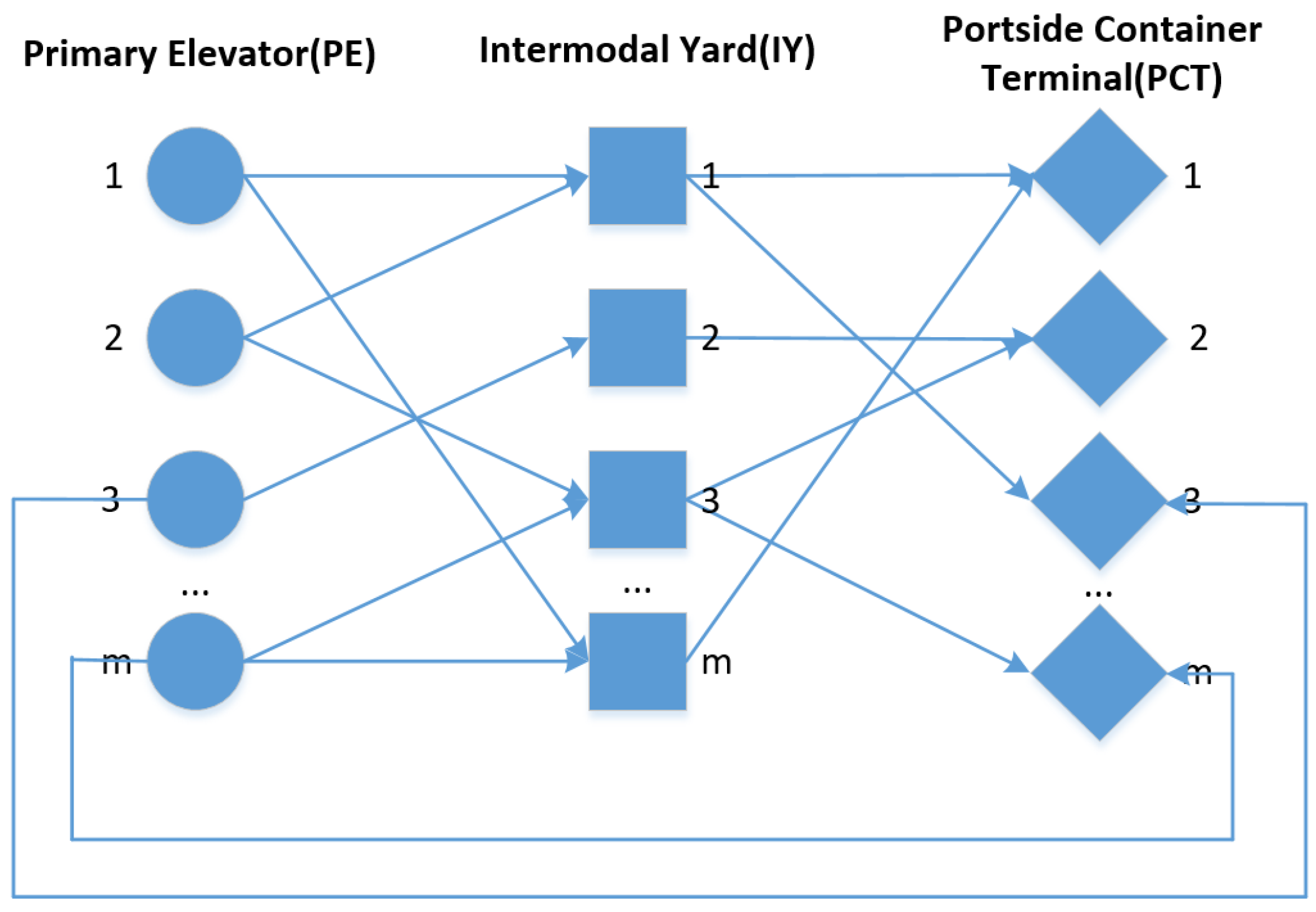
The optimal schedule with values for all decision variables, including the amount of inventory at all PEs and IYs, the total number of each type of trucks and wagons that was used for delivery at every given time period, the grain quantity shipped from all PEs to all IYs and PCTs, and the grain quantity shipped from all IYs to all PCTs, are shown in

Table 3. The optimal schedule of the simulated supply chain (inventory data; TEU stands for Twenty-foot Equivalent Unit).

Period	Site Type	Inventory at the Beginning of the Period, ton	Inventory at the End of the Period, ton	Inventory at the Beginning of the Period, TEU	Inventory at the End of the Period, TEU
$t_1$	m1	41,000	28,434	0	0
	m2	34,000	24,299	0	0
	m3	21,000	14,674	0	0
	m4	39,000	29,856	0	0
	m5	23,000	16,869	0	0
	s1	0	2513	0	100
	s2	0	5327	0	212
	s3	0	0	0	0
	s4	0	25	0	1
$t_2$	m1	28,434	20,844	0	0
	m2	24,299	15,208	0	0
	m3	14,674	9679	0	0
	m4	29,856	21,563	0	0
	m5	16,869	14,047	0	0
	s1	2513	10,806	100	430
	s2	5327	4523	212	180
	s3	0	301	0	12
	s4	25	25	1	1
$t_3$	m1	20,844	13,957	0	0
	m2	15,208	5306	0	0
	m3	9679	7026	0	0
	m4	21,563	19,904	0	0
	m5	14,047	7124	0	0
	s1	10,806	5428	430	216
	s2	4523	4925	180	196
	s3	301	301	12	12
	s4	25	25	1	1
$t_4$	m1	13,957	6971	0	0
	m2	5306	0	0	0
	m3	7026	0	0	0
	m4	19,904	15,028	0	0
	m5	7124	0	0	0
	s1	5428	0	216	0
	s2	4925	0	196	0
	s3	301	0	12	0
	s4	25	0	1	0

and

Table 4. The optimal schedule of the simulated supply chain (transportation data).

Period	The Beginning Site	The End Site	Shipped Grain Quantity, ton	Number of Containers Shipped, TEU	Number of Trucks $\left({\mathit{p}}_1\right)$	Number of Trucks $\left({\mathit{p}}_2\right)$	Number of Wagons $\left({\mathit{r}}_1\right)$
	m1	s2	5327	212	0	212	0
	m2	s2	9700	386	193	0	0
	m4	s1	9143	364	182	0	0
	m5	s4	38	2	1	0	0
	m1	n1	7238	288	144	0	0
$t_1$	m3	n3	6325	252	126	0	0
	m5	n1	6093	243	122	0	0
	s1	n2	6630	264	0	0	132
	s2	n1	3669	146	0	0	73
	s2	n2	1357	54	0	0	27
	s2	n3	4674	186	0	0	93
	s4	n2	25	1	0	0	1
	m2	s2	9091	362	181	0	0
	m3	s3	301	12	6	0	0
	m4	s1	8293	330	165	0	0
	m1	n1	6986	278	139	0	0
	m1	n2	603	24	12	0	0
	m3	n3	4693	187	94	0	0
	m5	n1	38	2	1	0	0
$t_2$	m5	n2	2808	112	56	0	0
	s2	n2	8588	342	0	0	171
	s2	n3	1306	52	0	0	26
	m2	s2	9902	394	197	0	0
	m4	s1	1658	66	33	0	0
	m1	n1	6886	274	137	0	0
	m3	n2	32	2	1	0	0
$t_3$	m3	n3	2621	105	53	0	0
	m5	n1	5113	204	102	0	0
	m5	n2	1810	72	36	0	0
	s1	n2	7037	280	0	0	140
	s2	n2	4121	164	0	0	82
	s2	n3	5378	214	0	0	107
	m2	s2	5306	212	106	0	0
	m4	s1	4876	194	97	0	0
	m1	n1	6987	278	139	0	0
	m3	n3	7026	280	140	0	0
	m5	n1	5013	200	100	0	0
	m5	n2	2111	84	42	0	0
$t_4$	s1	n2	10,304	410	0	0	205
	s2	n2	584	24	0	0	12
	s2	n3	9647	384	0	0	192
	s3	n3	301	12	0	0	6
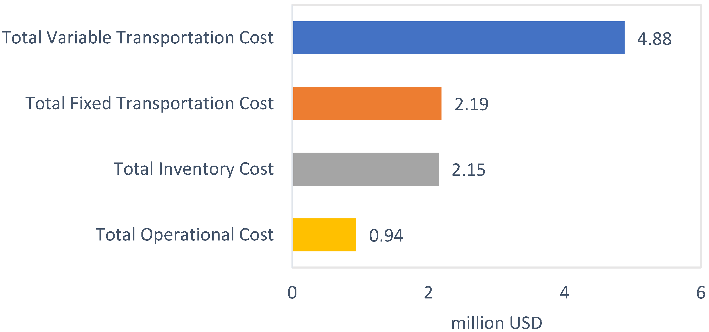
	s4	n3	25	1	0	0	1

. The optimal schedule minimizes the total cost of the supply chain, and the cost components’ values in the total cost of the supply chain are shown in Figure 4. The dominant share, about 69.7% (USD 7,066,197) of the total supply chain cost, is the transportation cost, and the second contributor to the total cost of the supply chain is the inventory cost, which accounts for 21.1% (USD 2,145,448), followed by the operational cost, which accounts for 9.2% (USD 937,057). To better understand the correlation between the simulation parameters and the total supply chain cost, and to discuss the possibilities of further minimization of the total supply chain cost, three main parts of the total supply chain cost should be discussed separately.

The transportation cost: Total transportation cost consists of a fixed transportation cost and a variable transplantation cost, which are influenced by many simulation parameters and variables. For instance, the fixed transportation cost is influenced by the number and type of trucks and wagons that are used for transportation and the fixed transportation cost per truck or wagon of different types. The variable transportation cost is shaped by the number and type of trucks and wagons that are used for transportation, the quantity of grain shipped, the weight of an empty container, the unit shipment cost, and the distance between the nodes of the supply chain. The data on the fixed transportation cost, the weight of an empty container, the unit shipment cost, and the distance between the nodes of the supply chain in this simulation were based on real-life data in Ukraine and taken from reliable sources. This is why we do not consider the changes in these parameters as a tool for minimizing the total cost that is worthy of further investigation. The number of trucks and wagons that are used for delivery can be limited by the number of trucks and wagons that are available at a site in a given period of time, the capacity of the IY used, and the quantity of grains that is available at the PE used.

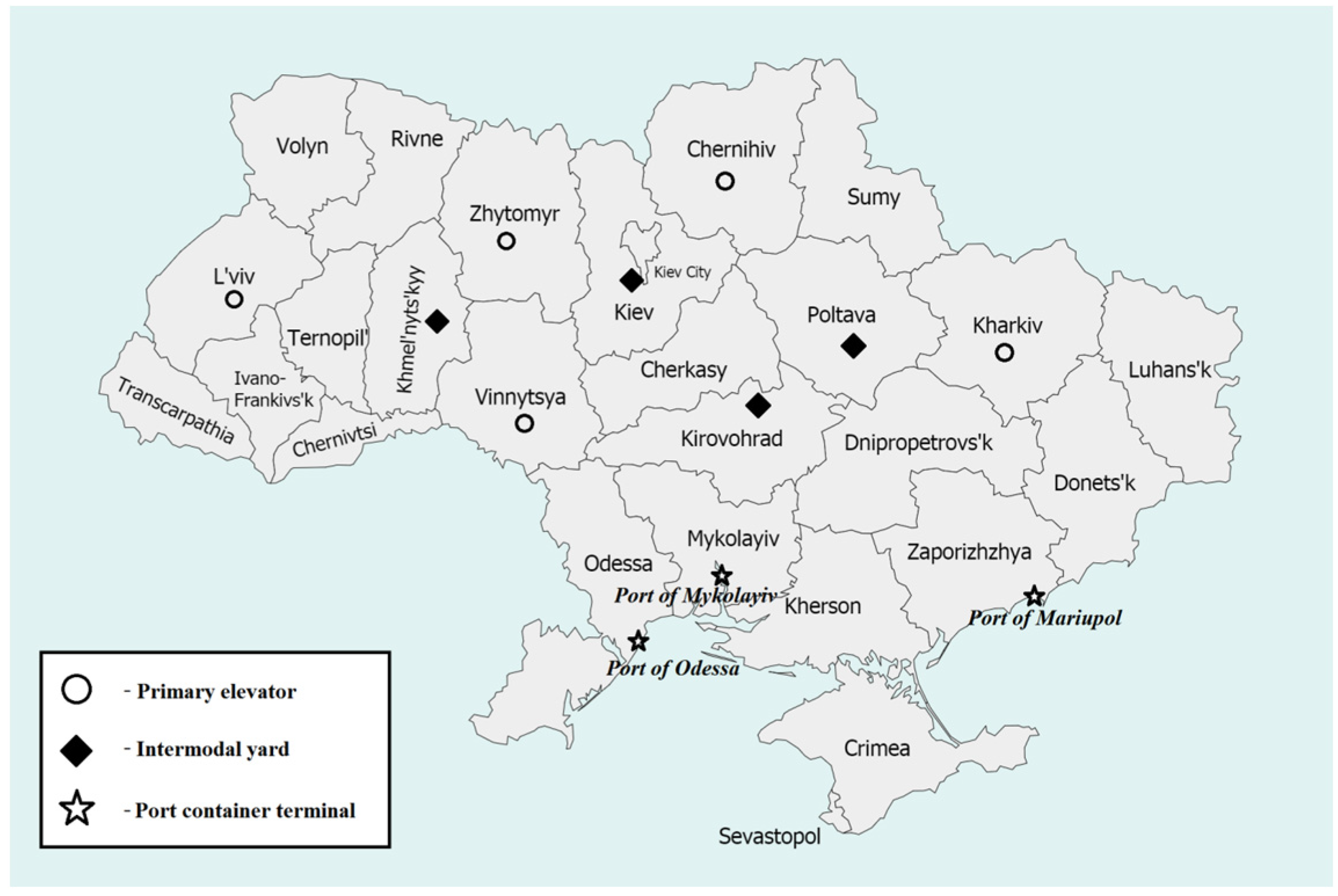
From the optimal schedule for this simulation, we can see that around 53.2% (72,372 tons) is transported by direct truck delivery from the PEs to PCTs, and only 46.8% (63,646 tons) is delivered through the IYs. This happens because direct delivery from the primary elevators that are located relatively close to the ports, such as $m_1$, $m_3$, and $m_5$, is a nice alternative to multi-modal delivery. The economic feasibility of direct delivery can be further proven by the fact that for 52.3% of the quantity of grains shipped, it only represents 50.8% (USD 3,587,285) of total transportation cost. Multimodal transportation, on the other hand, provides better cost for middle-long distances. For a share of 47.7% of the quantity of grains shipped, multimodal transportation’s share in the total transportation cost is 49.2% (USD 3,478,912); in addition, multimodal transportation creates additional sources of operational cost (loading and unloading) at the IYs. However, it should be mentioned that the capacity of the IYs and the number of wagons available at the IYs set an additional restriction on the quantity of grains that can be shipped through them. It is also clear that the model gives a preference to the usage of trucks with higher capacity $\left(p_1\right)$ as being more economically feasible. Only 212 containers are transported by trucks with lower capacity $\left(p_2\right)$. We can conclude that the number of trucks with higher capacity $\left(p_1\right)$ that are available at the PEs plays an important role in the transportation cost structure.

Based on the above results, we can conclude that the reasonable strategies to decrease the transportation cost of the supply chain are as follows:

• Increase the number of wagons that are available at the IYs to increase the outflow of the IYs.
• Increase the capacity of the IYs to increase the inflow of the IYs.
• Increase the number of trucks with high capacity $\left(p_1\right)$ that are available at the PEs, especially at those that are located relatively close to the PCTs.

The inventory holding cost: From the data that we used for the simulation, we can calculate the average inventory holding cost per container at the IYs and the average inventory holding cost of the bulk weight of a container with a full load of grains at the PEs. On average, it costs USD 134 to store a container at an IY for one quarter of the year, the same amount of grains as a full load of a container can be stored for one quarter of the year at a PE for USD 147. Even though inventory holding is cheaper, we need to take into account additional operational cost that comes with the use of multimodal transportation, which is the cost of unloading a container from a truck and loading it onto a wagon. This cost is applied to containers only once, regardless of the time that the containers spend in an IY. The average inventory holding cost and the cost of unloading and loading of a container at an IY is USD 137 for a container that has been stored for three months, which is 6.6% cheaper than the cost of storing the same amount of grains in bulk at the PE. However, the difference in cost will only increase with time duration since this additional operational cost occurs only once. On average, the storage of grains at an IY compared to the storage at a PE will be 7.7% cheaper for the duration of two quarters of the year, 8.1% for a storage period of three quarters, and 8.3% for a storage period of four quarters. This is the reason why the optimal schedule tries to deliver the scheduled quantity of grains as early as the capacitated number of vehicles at the PE and the capacity of the IY allow.

Based on the above results, we can conclude that the reasonable strategies to decrease the inventory holding cost of the supply chain are as follows:

• Increase the capacity of the IYs to increase the number of containers that can be stored and shipped through the IYs.
• Increase the number of trucks that are available at the PEs to make sure that grains are delivered to the IYs as early as possible.

The operational cost: The total operational cost has the smallest share in the total supply chain cost and affects the process of decision-making about the optimal schedule the least. In a primary elevator, a part of the operational cost occurs due to pricing, cleaning, weighting, sorting, blending, and quality control. This part of the operational cost occurs only once after grains are received by a PE from farms. Other sources of operational cost are the loading of bulk grains into containers and loading of containers onto trucks. The only sources of operational cost at the IYs and PCTs are the loading and unloading of containers to and from trucks and wagons. The only source of operational cost that varies depending on the schedule is the cost of loading and unloading of containers at the IYs. Therefore, it is hard to achieve significant changes in the operational cost simply by applying different schedules. In order to further minimize the operational cost without decreasing the quality and safety of products, processing facilities should be modernized, and staff training standards should be improved.

4.1.2. Disruption Management Model Simulation Results

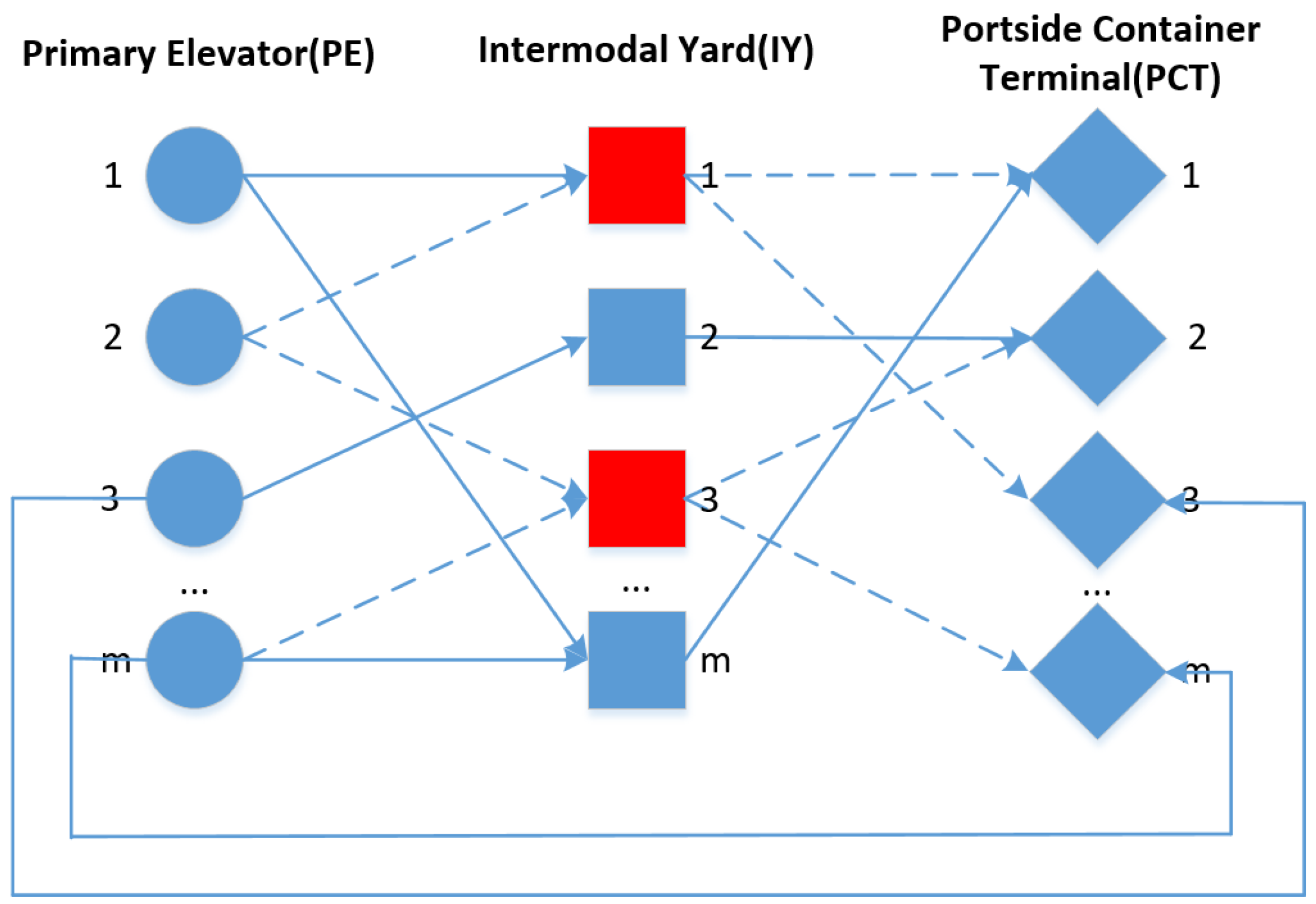
The value of the minimal expected total cost is provided, as well as the probability and minimal total cost of the supply chain for each disruption scenario. The list of disruption scenarios that were simulated, the probability of each disruption scenario, the minimal total cost of each disruption scenario, and the expected total cost of the supply chain are shown in

Table 5. The probability and minimal total cost of disruption scenarios (part 1).

Disruption Scenario	Disrupted IYs	Disruption Period	Probability	Minimal Total Cost, USD
No disruption	none	none	0.68908847	10,148,702
Disruption scenario №1	s1	t1	0.01882188	10,150,696
Disruption scenario №2	s1	t2	0.01882188	10,152,135
Disruption scenario №3	s1	t3	0.01882188	10,157,658
Disruption scenario №4	s1	t4	0.01882188	10,162,354
Disruption scenario №5	s2	t1	0.02852387	10,161,248
Disruption scenario №6	s2	t2	0.02852387	10,158,275
Disruption scenario №7	s2	t3	0.02852387	10,156,675
Disruption scenario №8	s2	t4	0.02852387	10,159,501
Disruption scenario №9	s3	t1	0.00931588	10,148,702
Disruption scenario №10	s3	t2	0.00931588	10,148,702
Disruption scenario №11	s3	t3	0.00931588	10,148,702
Disruption scenario №12	s3	t4	0.00931588	10,148,702
Disruption scenario №13	s4	t1	0.01882188	10,148,702
Disruption scenario №14	s4	t2	0.01882188	10,148,702
Disruption scenario №15	s4	t3	0.01882188	10,148,702
Disruption scenario №16	s4	t4	0.01882188	10,148,702
Disruption scenario №17	s1, s2	t1	0.00058211	10,160,061
Disruption scenario №18	s1, s2	t2	0.00058211	10,157,865
Disruption scenario №19	s1, s2	t3	0.00058211	10,159,963
Disruption scenario №20	s1, s2	t4	0.00058211	10,175,641
Disruption scenario №21	s1, s3	t1	0.00019012	10,153,707
Disruption scenario №22	s1, s3	t2	0.00019012	10,150,649
Disruption scenario №23	s1, s3	t3	0.00019012	10,152,500
Disruption scenario №24	s1, s3	t4	0.00019012	10,166,564
Disruption scenario №25	s1, s4	t1	0.00038412	10,154,153
Disruption scenario №26	s1, s4	t2	0.00038412	10,149,783
Disruption scenario №27	s1, s4	t3	0.00038412	10,153,563
Disruption scenario №28	s1, s4	t4	0.00038412	10,163,605
Disruption scenario №29	s2, s3	t1	0.00028812	10,155,796
Disruption scenario №30	s2, s3	t2	0.00028812	10,158,416

and

Table 6. The probability and minimal total cost of disruption scenarios (part 2).

Disruption Scenario	Disrupted IYs	Disruption Period	Probability	Minimal Total Cost, USD
Disruption scenario №31	s2, s3	t3	0.00028812	10,159,466
Disruption scenario №32	s2, s3	t4	0.00028812	10,160,112
Disruption scenario №33	s2, s4	t1	0.00058212	10,156,068
Disruption scenario №34	s2, s4	t2	0.00058212	10,162,601
Disruption scenario №35	s2, s4	t3	0.00058212	10,156,989
Disruption scenario №36	s2, s4	t4	0.00058212	10,159,922
Disruption scenario №37	s3, s4	t1	0.00019012	10,148,702
Disruption scenario №38	s3, s4	t2	0.00019012	10,148,702
Disruption scenario №39	s3, s4	t3	0.00019012	10,148,702
Disruption scenario №40	s3, s4	t4	0.00019012	10,148,702
Disruption scenario №41	s1, s2, s3	t1	0.00000588	10,160,436
Disruption scenario №42	s1, s2, s3	t2	0.00000588	10,157,898
Disruption scenario №43	s1, s2, s3	t3	0.00000588	10,162,106
Disruption scenario №44	s1, s2, s3	t4	0.00000588	10,173,592
Disruption scenario №45	s1, s2, s4	t1	0.00001199	10,161,014
Disruption scenario №46	s1, s2, s4	t2	0.00001199	10,159,644
Disruption scenario №47	s1, s2, s4	t3	0.00001199	10,159,425
Disruption scenario №48	s1, s2, s4	t4	0.00001199	10,180,434
Disruption scenario №49	s1, s3, s4	t1	0.00000388	10,149,594
Disruption scenario №50	s1, s3, s4	t2	0.00000388	10,149,088
Disruption scenario №51	s1, s3, s4	t3	0.00000388	10,152,594
Disruption scenario №52	s1, s3, s4	t4	0.00000388	10,164,424
Disruption scenario №53	s2, s3, s4	t1	0.00000588	10,159,008
Disruption scenario №54	s2, s3, s4	t2	0.00000588	10,157,382
Disruption scenario №55	s2, s3, s4	t3	0.00000588	10,155,424
Disruption scenario №56	s2, s3, s4	t4	0.00000588	10,163,164
Disruption scenario №57	s1, s2, s3, s4	t1	0.00000012	10,161,374
Disruption scenario №58	s1, s2, s3, s4	t2	0.00000012	10,158,885
Disruption scenario №59	s1, s2, s3, s4	t3	0.00000012	10,159,247
Disruption scenario №60	s1, s2, s3, s4	t4	0.00000012	10,175,507
Expected total cost of the supply chain		10,150,483

. The simulation considering disruptions that can occur at four IYs and at any point of four existing time periods leads to 50% loss in the capacity of the IYs in a given period of time. In case of a disruption in the previous time period, an IY will be able to recover its capacity in this time period since one time period, which is three-month long, provides an adequate amount of time to solve most of the possible disruption causes. All disruption cases can be described by 61 disruption scenarios. Each disruption scenario represents a unique subset of IYs that are currently disrupted and those that are working without disruption in a given period of time.

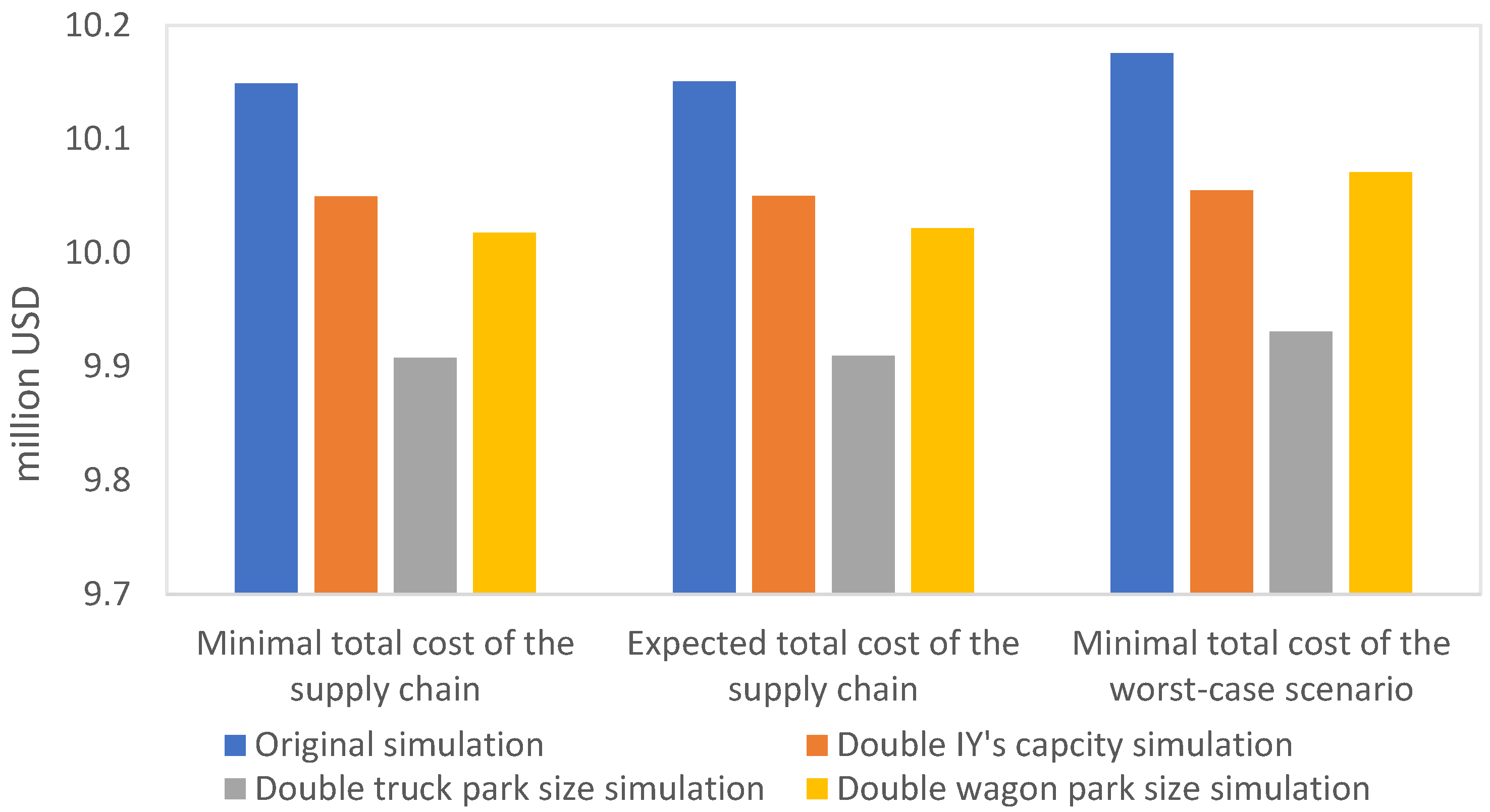
The expected total cost of the supply chain is USD 10,150,483, which is only 0.018% (USD 1781) greater than the minimal total cost of the supply chain that operates without disruption. Moreover, the minimal total cost of the worst-case scenario (scenario №60) with disruption at all IYs during the fourth time period is USD 10,175,507, which is only 0.26% (USD 26,805) more expensive than the minimal total cost of the supply chain that operates without disruption. The disruption scenario №60 provides us the highest total cost because all IYs are disrupted during a period of time with the highest demand out of the four time periods—41,000 tons—compared to the demand of time period three at 33,000 tons, time period two at 25,000 tons, and time period one at 36,000 tons. Because the IYs are only working at 50% of their actual capacity, the supply chain cannot fully exploit the benefits of the comparably cheaper railway delivery over long distances and the lower inventory cost of the IYs. However, the overall total cost is only raised by 0.26%, which is proof of the high sustainability of the proposed supply chain. The robustness of the supply chain is ensured by the possibility of direct truck delivery, the high quantity of grain suppliers (PEs) and IYs that are spread widely across the country, and the compatibility of the costs of short-distance truck delivery and multimodal delivery over long distances.

4.2. Sensitivity Analysis

The sensitivity analysis mainly focused on the cost minimization strategies that were proposed in Section 4.1.1 and aimed to analyze the effect of these strategies on the minimal total cost of the supply chain and the sustainability of the supply chain. The results of the simulations were compared with the results of the original model simulations. Graphic representation of the findings of the sensitivity analysis simulations and the original model simulation is shown in Figure 5.

4.2.1. Effect of Intermodal Yard Capacity

The data that were used for this simulation were drawn from the original simulation, but the capacity of all IYs in the supply chain was doubled for this simulation. We can see that an increase in the IYs’ capacity leads to a reduction in the minimal total cost of the supply chain by 1% (USD 101,348), as shown in Figure 5. The worst-case scenario increases the minimal total cost of the supply chain only by 0.056% (USD 5585), compared to the 0.26% increase in the original simulation. The expected total cost of the supply chain is 0.005% (USD 505) greater than the minimal total cost of the supply chain that operates without disruption, compared to the 0.018% increase in the original simulation.

Based on the findings of the simulation, we can conclude that an increase in the intermodal yard capacity have a positive effect on the cost formulation of the supply chain and the sustainability of the supply chain.

4.2.2. Effect of Wagon Park Size on Intermodal Yard

The data that were used for this simulation were drawn from the original simulation, but the number of available wagons at the IYs for each time period was doubled for this simulation. The simulation results suggest that by doubling the number of wagons at the IYs, we can decrease the minimal total cost of the supply chain by 1.3% (USD 131,242). The expected total cost of the supply chain is 0.043% (USD 4318) greater than the minimal total cost of the supply chain that operates without disruption, compared to the 0.018% increase in the original simulation. The worst-case scenario increases the minimal total cost of the supply chain only by 0.53% (USD 53,164), compared to the 0.26% increase in the original simulation. From the results of the simulation, we can see that increasing wagon park size actually increases the influence of disruption on the overall performance of the supply chain. The reason behind this is the increase in the multimodal transportation share in the total amount of grains shipped. In the original simulation that operates without disruption, around 52.3% of the total quantity of grains is shipped using direct delivery and 47,7% is shipped using multimodal transportation. After the increase in the number of wagons, the share of direct transplantation is lowered to 33.6% (45,721 tons), and the share of multimodal transportation rises to 66.4% (90,279 tons). When an IY loses its capacity due to disruption, it also significantly effects the outflow of the IY; the higher the share of multimodal transportation in the total amount of grains shipped, the higher the effect of the IY disruption on the supply chain system. However, the losses that a company might suffer due to disruption are insignificant compared to the total cost of the supply chain, even in the worst-case scenario.

Based on the finding of the simulation, we can conclude that an increase in the wagon park size of an IY not only has a positive effect on the cost formulation but also increases the effect of disruption on the supply chain.

4.2.3. Effect of Truck Park Size on Primary Elevator

The data that were used for this simulation were drawn from the original simulation, but the number of trucks of each type at all PEs was doubled for each time period. Doubling the number of trucks at the PEs leads to a reduction in the minimal total cost of the supply chain by 2.4% (USD 240,819). The worst-case scenario increases the minimal total cost of the supply chain by 0.23% (USD 22,920), compared to the 0.26% increase in the original simulation. The expected total cost of the supply chain is 0.015% (USD 1475) greater than the minimal total cost of the supply chain that operates without disruption, compared to the 0.018% increase in the original simulation. It should also be mentioned that because the supply of larger trucks $\left(p_1\right)$ exceeded the demand, smaller trucks $\left(p_2\right)$ were not used for delivery in this simulation.

Based on the findings of the simulation, we can conclude that an increase in the truck park size of an IY has a positive effect on the cost formulation and the sustainability of the supply chain.

5. Conclusions

In recent years, more and more countries are starting to consider container transportation as an alternative to bulk shipment of grains. To date, no meaningful study has been conducted to examine containerized grain transportation problem in Ukraine. To fill this research gap, this study addresses the containerized grain transportation problem in Ukraine while considering disruption scenarios that can occur at intermodal yards. This research creates a supply chain system that delivers grains in containers from a primary elevator to a port container terminal through an intermodal yard, while considering the possibility of direct delivery of grains from the primary elevator to the port container terminal. To achieve the objective of this study, two mathematical models were developed. The containerize grain transportation model was developed to minimize the total cost of the containerized grain supply chain, including the total transportation cost of road and railway transportation, the operational costs of primary elevators, intermodal yards, and port container terminals, and the inventory holding costs of primary elevators and intermodal yards. The disruption management model that minimizes the expected total cost of the supply chain while considering disruption scenarios that can occur at intermodal yards at any given time period leads to 50% loss in the capacity of the intermodal yards at the given period of time. The linear programing models incorporate multi-period, direct and multi-modal transportation, vehicle and container capacity, bulk and container inventory holding, and demand satisfaction restrictions.

A containerized grain supply chain that consists of five primary elevators, four intermodal yards, and three port container terminals was suggested for the model’s simulation. Python software with the SCIP solver was used to solve the proposed mathematical models. The results of the containerized grain transportation model simulation provide a schedule that minimizes the total cost of the supply chain. They also show that the dominant contributor to the supply chain total cost is the transportation cost. It is also clear that the model gives a preference to the usage of trucks with higher capacity $\left(p_1\right)$ as being more economically feasible. Another finding of the simulation is that the optimal schedule tries to deliver the scheduled quantity of grains to an intermodal yard as early as the capacitated number of vehicles at the primary elevators and the capacity of the intermodal yard allow due to the fact that the storage of containerized grains is cheaper than bulk storage at the primary elevators. The results of the other model considering disruption scenarios show that the simulated supply chain has a high level of sustainability. The robustness of the supply chain is ensured by the possibility of direct truck delivery, the high quantity of grain suppliers (primary elevators) and intermodal yards that are spread widely across the country, and the compatibility of the costs of short-distance truck delivery and multimodal delivery over long distances. Sensitivity analysis was conducted by changing the models’ parameters. The sensitivity analysis focused on the proposed cost minimization strategies and aimed to analyze the effect of these strategies on the minimal total cost of the supply chain and the sustainability of the supply chain. The results of the sensitivity analysis show that an increase in the intermodal yard capacity and in the truck park size have a positive effect on the cost formulation of the supply chain and the sustainability of the supply chain. An increase in the wagon park size of an IY not only has a positive effect on the cost formulation but also increases the effect of disruption on the supply chain.

The proposed models consider the deterministic nature of procurement and demand, and future studies can be extended by considering stochastic procurement and demand. The scope of this study can be further expanded to the delivery of grains to final customers, including the sea shipment process and transportation of grain from a receiving port to a customer. Containerized multi-grain supply chain optimization is another possible research direction. Transportation time with due dates and a penalty system that is applied in case of shipment delay can be added to the disruption management model. Additionally, in order to create a better green and sustainable grain logistics system, we can consider CO₂ emissions as an objective function.

References

1. Kim, Y.J.; Lee, B.K. Containerized Grain Logistics Processes for Implementing Sustainable Identity Preservation. Sustainability 2022, 14, 13352. [Google Scholar] [CrossRef]
2. Maiyar, L.M.; Thakkar, J.J. Environmentally Conscious Logistics Planning for Food Grain Industry Considering Wastages Employing Multi Objective Hybrid Particle Swarm Optimization. Transp. Res. Part E Logist. Transp. Rev. 2019, 127, 220–248. [Google Scholar] [CrossRef]
3. Meng, X. The Analysis of the Motivation and Conditions of the “Scattered Change Set” Cargo. IOP Conf. Ser. Earth Environ. Sci. 2020, 546, 032038. [Google Scholar] [CrossRef]
4. Larina, T.; Kravcov, A.; Berezhnaja, N.; Kutiya, O.; Fenenko, K. Implementation of Logistic Approaches in Forming the Agricultural Export Strategy in Ukraine. J. Sustain. Dev. Transp. Logist. 2019, 4, 17–24. [Google Scholar] [CrossRef]
5. Pavlenko, O.; Automobile, K.N. The Choice of Rational Technology of Delivery of Grain Cargoes in the Containers in the International Traffic. Int. J. Traffic Transp. Eng. 2017, 7, 164–176. [Google Scholar]
6. Kovalov, A.; Prodashchuk, S.; Kravets, A.; Mkrtychian, D.; Prodashchuk, M. Improvement of the Grain Cargo Handling Technology on the Basis of Resource-Saving. IOP Conf. Ser. Mater. Sci. Eng. 2021, 1021, 012006. [Google Scholar] [CrossRef]
7. Ahumada, O.; Villalobos, J.R. Application of Planning Models in the Agri-Food Supply Chain: A Review. Eur. J. Oper. Res. 2009, 196, 1–20. [Google Scholar] [CrossRef]
8. Ahumada, O.; Villalobos, J.R. Operational Model for Planning the Harvest and Distribution of Perishable Agricultural Products. Int. J. Prod. Econ. 2011, 133, 677–687. [Google Scholar] [CrossRef]
9. Asgari, N.; Farahani, R.Z.; Rashidi-Bajgan, H.; Sajadieh, M.S. Developing Model-Based Software to Optimise Wheat Storage and Transportation: A Real-World Application. Appl. Soft Comput. J. 2013, 13, 1074–1084. [Google Scholar] [CrossRef]
10. Agustina, D.; Lee, C.K.M.; Piplani, R. Vehicle Scheduling and Routing at a Cross Docking Center for Food Supply Chains. Int. J. Prod. Econ. 2014, 152, 29–41. [Google Scholar] [CrossRef]
11. Maiyar, L.M.; Thakkar, J.J.; Awasthi, A.; Tiwari, M.K. Development of an Effective Cost Minimization Model for Food Grain Shipments. IFAC-Papersonline 2015, 28, 881–886. [Google Scholar] [CrossRef]
12. Lamsal, K.; Jones, P.C.; Thomas, B.W. Harvest Logistics in Agricultural Systems with Multiple, Independent Producers and No on-Farm Storage. Comput. Ind. Eng. 2016, 91, 129–138. [Google Scholar] [CrossRef]
13. Mogale, D.G.; Kumar, S.K.; Márquez, F.P.G.; Tiwari, M.K. Bulk Wheat Transportation and Storage Problem of Public Distribution System. Comput. Ind. Eng. 2017, 104, 80–97. [Google Scholar] [CrossRef]
14. Gholamian, M.R.; Taghanzadeh, A.H. Integrated Network Design of Wheat Supply Chain: A Real Case of Iran. Comput. Electron. Agric. 2017, 140, 139–147. [Google Scholar] [CrossRef]
15. Mogale, D.G.; Kumar, M.; Kumar, S.K.; Tiwari, M.K. Grain Silo Location-Allocation Problem with Dwell Time for Optimization of Food Grain Supply Chain Network. Transp. Res. Part E Logist. Transp. Rev. 2018, 111, 40–69. [Google Scholar] [CrossRef]
16. Wagner, S.M.; Bode, C. An Empirical Examination of Supply Chain Performance Along Several Dimensions of Risk. J. Bus. Logist. 2008, 29, 307–325. [Google Scholar] [CrossRef]
17. Passarelli, M.; Bongiorno, G.; Beraldi, P.; Musmanno, R.; Filice, L. Supply Chain Management in Case of Producer Disruption between External (Instable) Forces and Effective Models. Procedia Comput. Sci. 2023, 217, 1305–1315. [Google Scholar] [CrossRef]
18. Rodrigues, V.S.; Stantchev, D.; Potter, A.; Naim, M.; Whiteing, A. Establishing a Transport Operation Focused Uncertainty Model for the Supply Chain. Int. J. Phys. Distrib. Logist. Manag. 2008, 38, 388–411. [Google Scholar] [CrossRef]
19. Janová, J. Crop Plan Optimization under Risk on a Farm Level in the Czech Republic. Agric. Econ. 2014, 60, 123–132. [Google Scholar] [CrossRef]
20. Tsiakis, P.; Shah, N. Design of Multi-Echelon Supply Chain Networks under Demand Uncertainty Design of Multi-Echelon Supply Chain Networks under Demand. Ind. Eng. Chem. Res. 2016, 40, 3585–3604. [Google Scholar] [CrossRef]
21. Svensson, G. A Conceptual Framework for the Analysis of Vulnerability in Supply Chains. Int. J. Phys. Distrib. Logist. Manag. 2000, 30, 731–750. [Google Scholar] [CrossRef]
22. Svensson, G. A Conceptual Framework of Vulnerability in Firms’ Inbound and Outbound Logistics Flows. Int. J. Phys. Distrib. Logist. Manag. 2002, 32, 110–134. [Google Scholar] [CrossRef]
23. Brockner, J.; Erika, H.J. Toward an Understanding of When Executives See Crisis as Opportunity. J. Appl. Behav. Sci. 2008, 44, 94–115. [Google Scholar] [CrossRef]
24. Braunscheidel, M.J.; Suresh, N.C. The Organizational Antecedents of a Firm’s Supply Chain Agility for Risk Mitigation and Response. J. Oper. Manag. 2009, 27, 119–140. [Google Scholar] [CrossRef]
25. Zsidisin, G.A.; Smith, M.E. Managing Supply Risk with Early Supplier Involvement: A Case Study and Research Propositions. J. Supply Chain Manag. 2005, 41, 44–57. [Google Scholar] [CrossRef]
26. Yang, Y.; Xu, X. Post-Disaster Grain Supply Chain Resilience with Government Aid. Transp. Res. Part E Logist. Transp. Rev. 2015, 76, 139–159. [Google Scholar] [CrossRef]
27. Craighead, C.W.; Blackhurst, J.; Rungtusanatham, M.J.; Handfield, R.B. The Severity of Supply Chain Disruptions: Design Characteristics and Mitigation Capabilities. Decis. Sci. 2007, 38, 131–156. [Google Scholar] [CrossRef]
28. Mudrageda, M.; Murphy, F.H. Designing Safety Space in a Supply Chain to Handle System-Wide Disruptions. Nav. Res. Logist. 2007, 54, 258–264. [Google Scholar] [CrossRef]
29. Su, Y.; Xie, K.; Wang, H.; Liang, Z.; Art Chaovalitwongse, W.; Pardalos, P.M. Airline Disruption Management: A Review of Models and Solution Methods. Engineering 2021, 7, 435–447. [Google Scholar] [CrossRef]
30. Van Kessel, P.J.; Freeman, F.C.; Santos, B.F. Airline Maintenance Task Rescheduling in a Disruptive Environment. Eur. J. Oper. Res. 2023, 308, 605–621. [Google Scholar] [CrossRef]
31. Wendler-Bosco, V.; Nicholson, C. Port Disruption Impact on the Maritime Supply Chain: A Literature Review. Sustain. Resilient Infrastruct. 2020, 5, 378–394. [Google Scholar] [CrossRef]
32. Hatefi, S.M.; Jolai, F. Robust and Reliable Forward-Reverse Logistics Network Design under Demand Uncertainty and Facility Disruptions. Appl. Math. Model. 2014, 38, 2630–2647. [Google Scholar] [CrossRef]
33. Hakelius, K.; Nilsson, J. The Logic behind the Internal Governance of Sweden’s Largest Agricultural Cooperatives. Sustainability 2020, 12, 9073. [Google Scholar] [CrossRef]
34. Ries, M. The COVID-19 Infodemic: Mechanism, Impact, and Counter-Measures—A Review of Reviews. Sustainability 2022, 14, 2605. [Google Scholar] [CrossRef]
Figure 1. Depiction of the transportation problem.
Sustainability 15 07620 g001
Figure 2. Depiction of the disruption management problem.
Sustainability 15 07620 g002
Figure 3. Locations of primary elevators, intermodal yards, and port container terminals.
Sustainability 15 07620 g003
Figure 4. Cost components’ values in the total cost of the supply chain.
Sustainability 15 07620 g004
Figure 5. The sensitivity analysis simulation results.
Sustainability 15 07620 g005