
Slope Failure Risk Assessment Considering Both the Randomness of Groundwater Level and Soil Shear Strength Parameters

Abstract
:1. Introduction
2. Methodologies
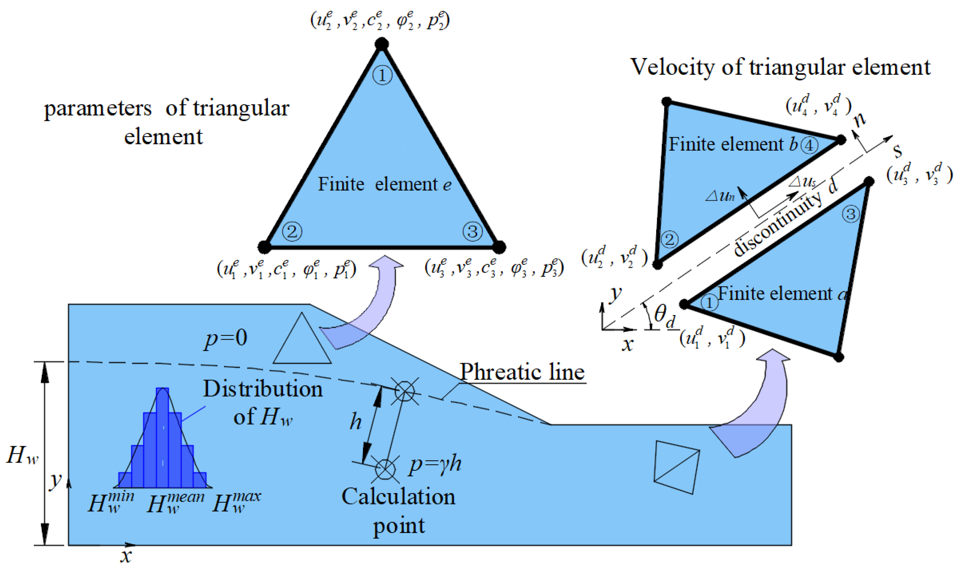
2.1. Stable Seepage Field of Slope with Stochastic Groundwater Level
2.2. Stochastic Field of Parameter Spatial Variability
2.3. Stochastic Programming Model
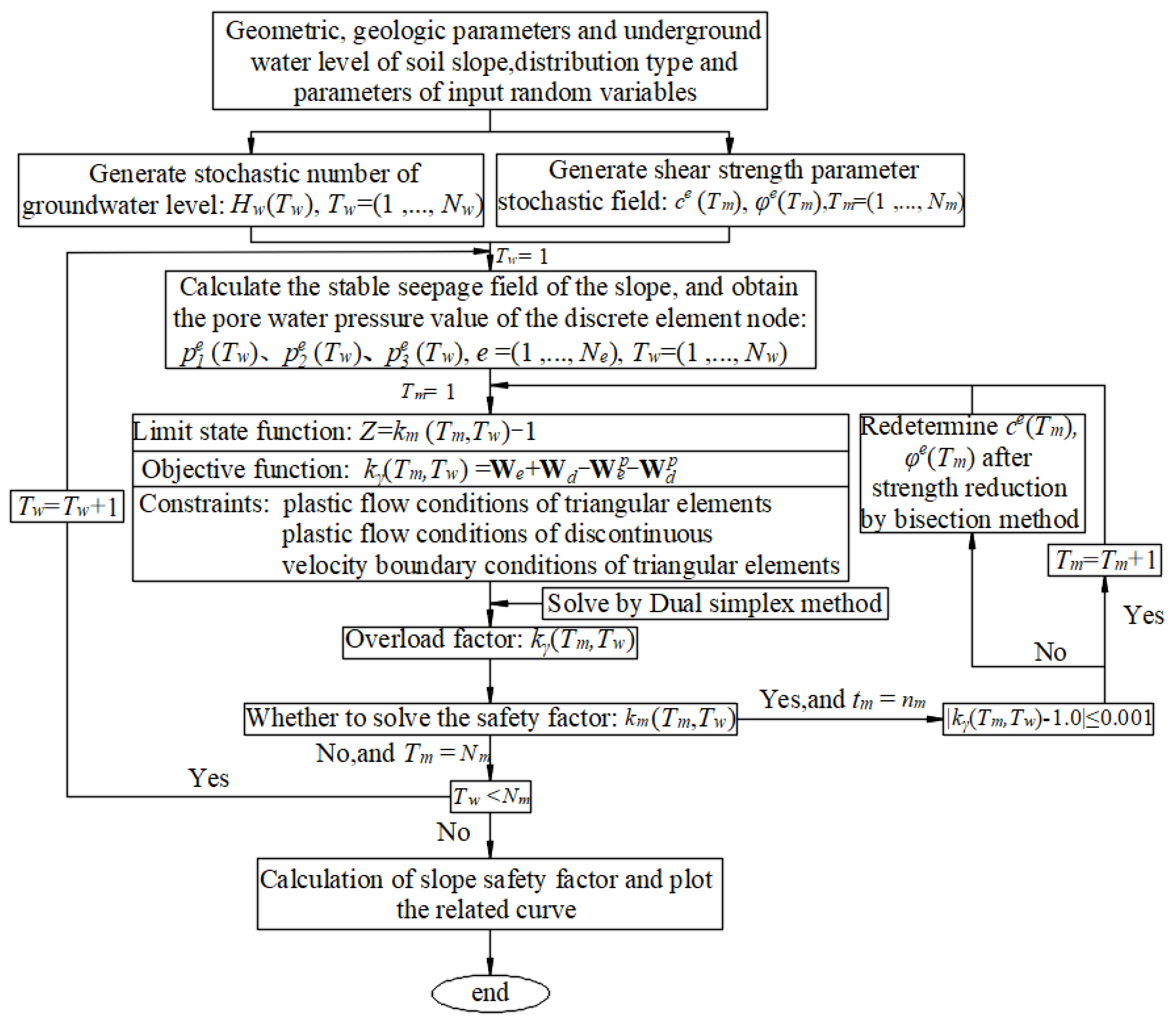
3. Solution Strategy
- (1)
- Assuming that the stochastic groundwater level follows a truncated normal distribution, which is generated with the Monte Carlo simulation method:where is the th groundwater level; , is the number of groundwater level; and and are the mean and standard deviation of the groundwater level, respectively.
- (2)
- Assuming that the autocorrelation functions of the soil materials are exponential type, using Equations (3) and (4), the midpoint method of Cholesky decomposition for the stochastic field generation and , of which ; is the number of random fields for the shear strength parameters.
- (3)
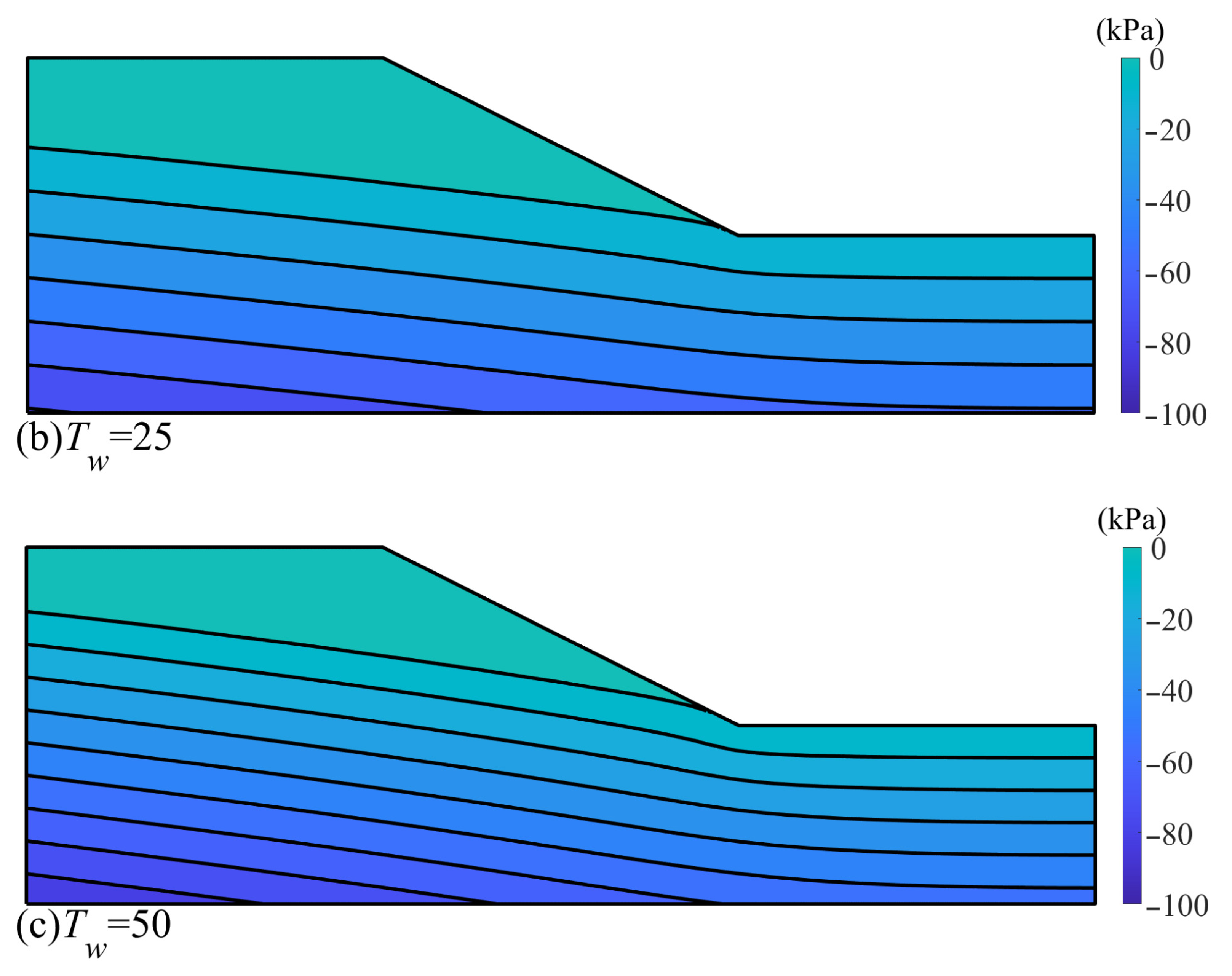
- The stochastic number of groundwater levels generated in step (1) is substituted into the stable seepage field calculation equation to obtain the pore water pressure , , ; ; .
- (4)
- From to cycles, repeat , , , all the finite element nodes’ pore water pressure values are successively replaced with the stochastic programming model for the slope reliability analysis; in each cycle from to ; , from to cycles, the number of stochastic fields are brought into Equation (5) and use the dual simplex method to obtain numbers of capacity overload factors while, at the same time, use the bisection method to obtain numbers of the slope safety factor . Figure 2 shows the specific numerical solution flow.
- (5)
- Calculation of the slope safety factor and plot the related curve.
4. Reliability Index for Slope
5. Calibration and Application
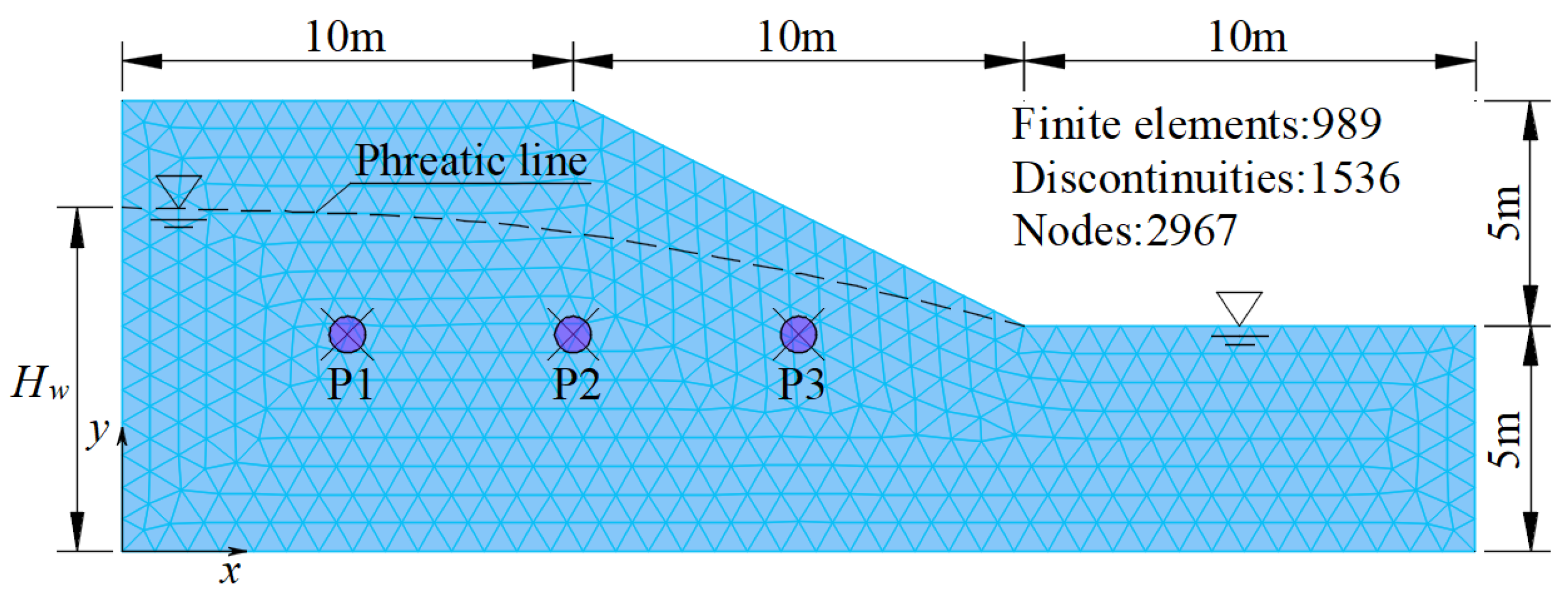
5.1. Numerical Simulations
5.2. Main Results of the Research
- (1)
- When , , and , the mean of the slope safety factors with the UBM is larger than that of the LEM, but the error is small, which conforms to the features of the upper bound solution. In addition, the slope safety factors acquired with the UBM and LEM methods decrease as the groundwater level rises. The slope failure probability increases acquired with the UBM and LEM decrease as the groundwater level rises. On the basis of the upper bound theorem, the slope safety factor acquired with the UBM must be greater than the real solution. Therefore, the UBM will slightly underestimate the failure slope probability.
- (2)
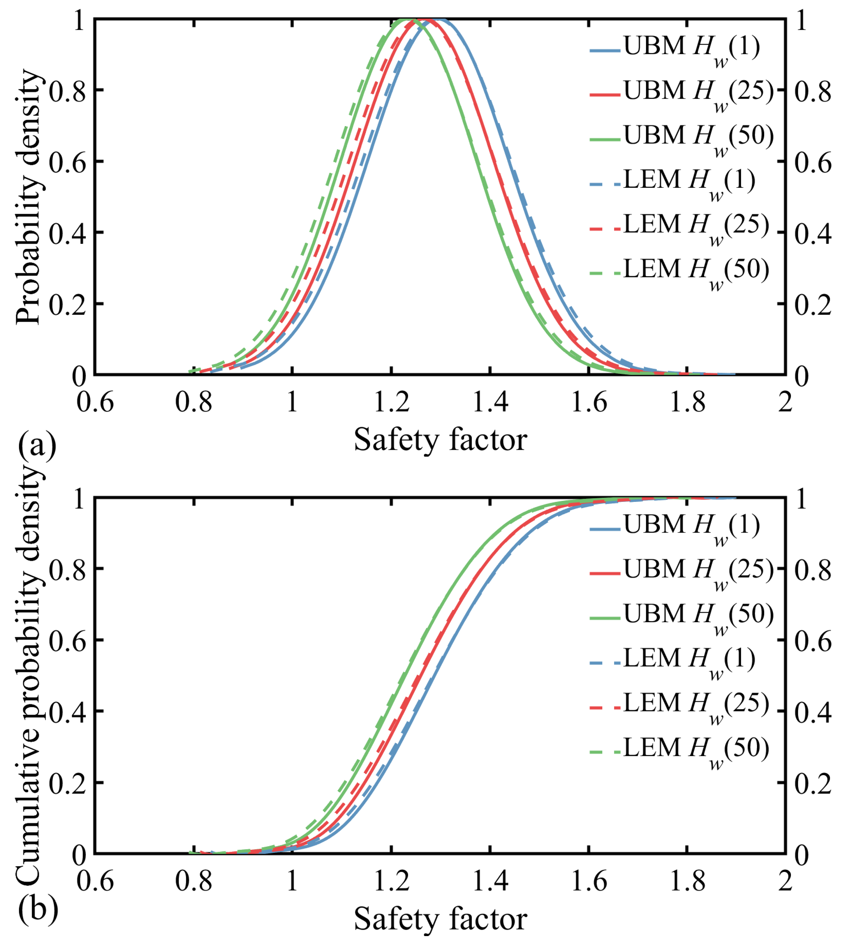
- Figure 8a,b shows the PDF and CDF curves of the slope safety factors acquired with the UBM and LEM under three groundwater level acts, , , and , respectively. It is not difficult to see that the PDF and CDF curves of the slope safety factors acquired with the UBM and LEM are very close with small errors. In addition, the PDF and CDF curves gradually move to the left as the groundwater level rises.
- (3)
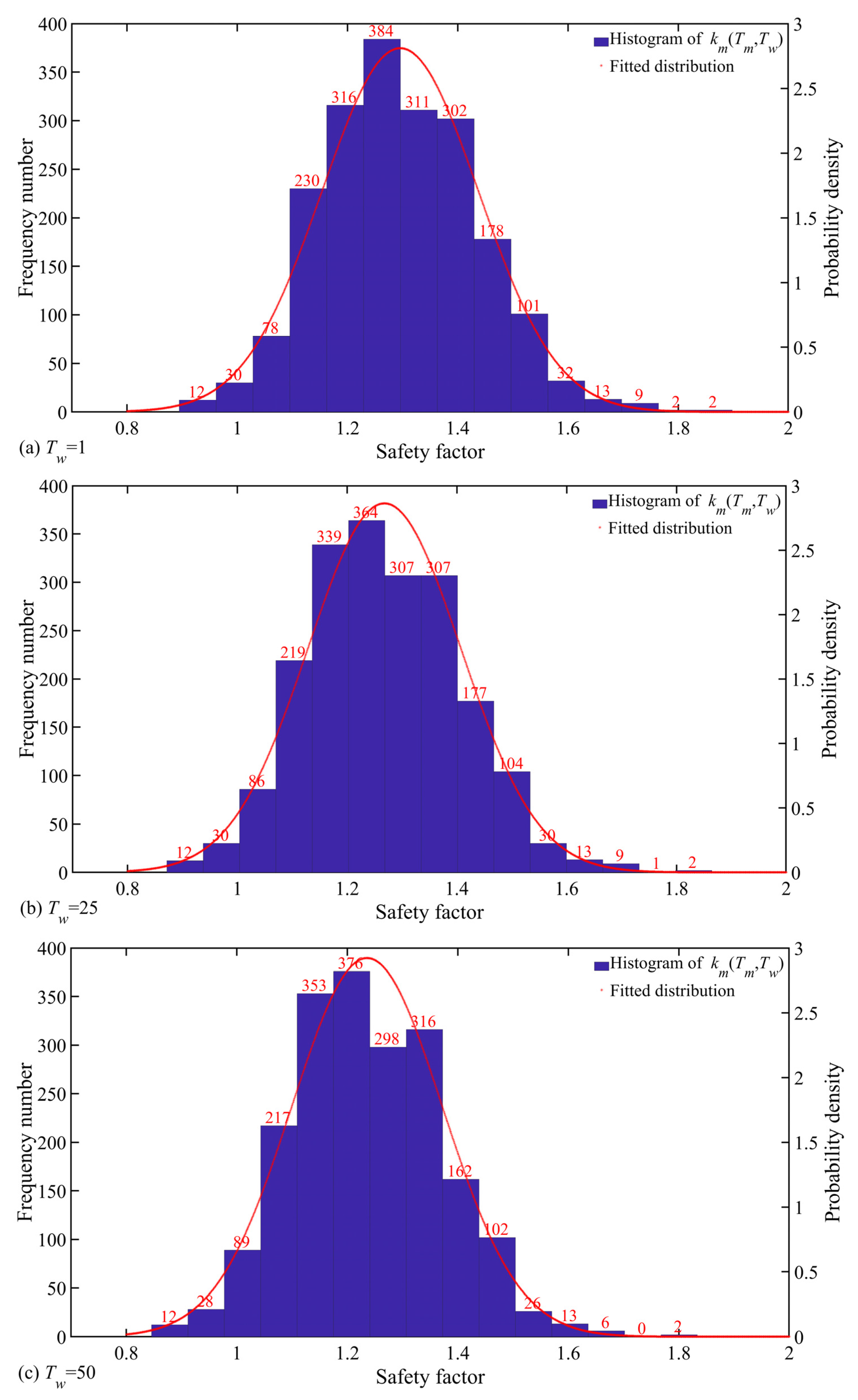
- Figure 9a–c are the distribution histograms of the slope safety factors acquired with the UBM under the three groundwater level acts, , , and , respectively. It is not difficult to see that the distribution of the slope safety factors is similar to the stochastic groundwater levels.
- (1)
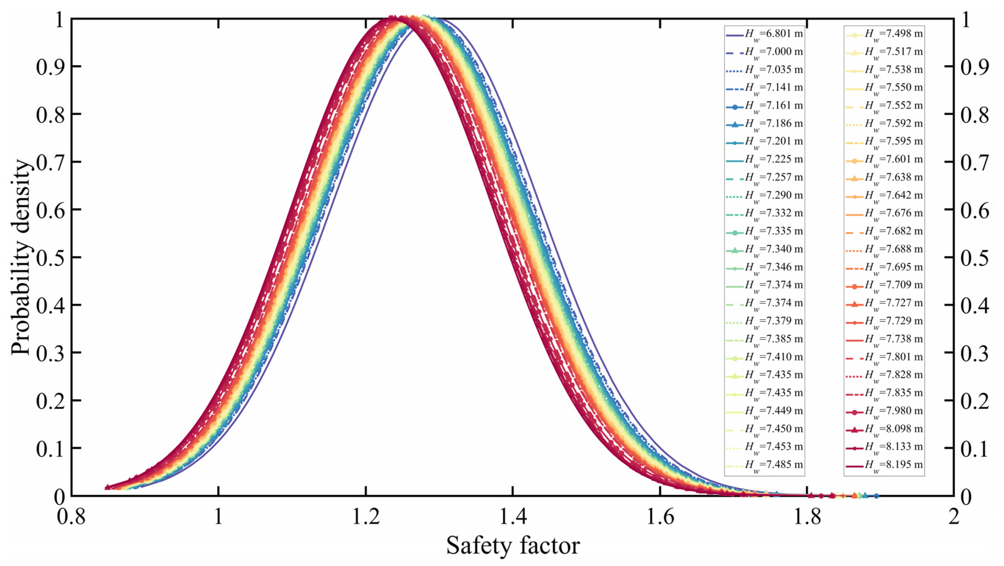
- The distribution of the slope safety factors is consistent with the normal distribution. The mean of the slope safety factors tends to decrease as the groundwater level rises. The PDF and CDF curves of the slope safety factors gradually move to the left as the groundwater level rises. In addition, the standard deviation of the slope safety factor tends to decrease as the groundwater level rises. The range of the PDF curve and the trend of the CDF curve of the slope safety factors gradually narrow and steepen, respectively.
- (2)
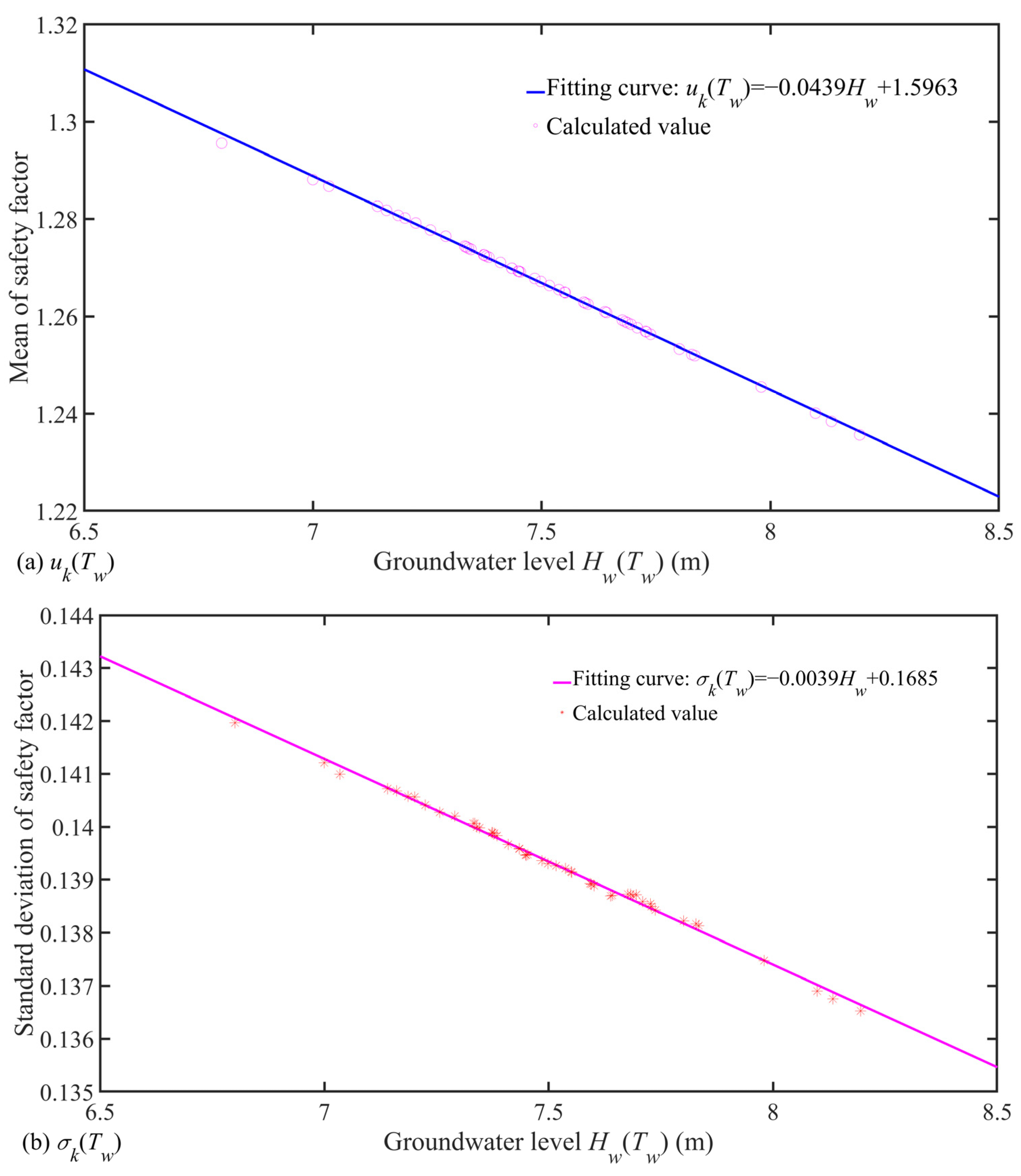
- A polynomial fit is used to acquire the quantitative equation of the mean and standard deviation of the slope safety factors and groundwater level as follows:
- (3)
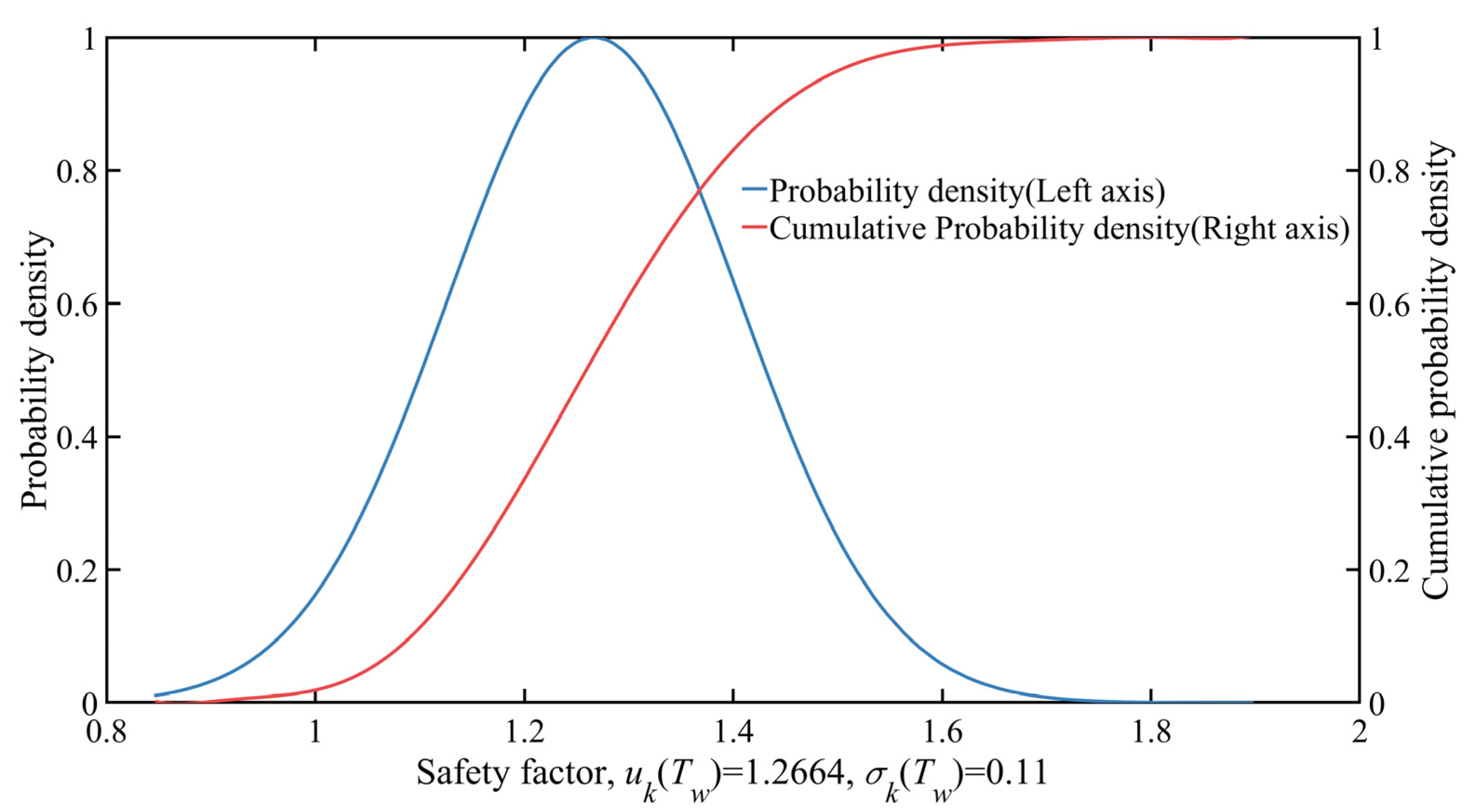
- The quantity of 100,000 slope safety factors was acquired from 2000 stochastic fields under 50 groundwater level acts to perform the statistical analysis of all the acquired data; under 50 groundwater level acts, the mean and standard deviation of the slope safety factors are 1.2664 and 0.11, respectively.
6. Conclusions
- (1)
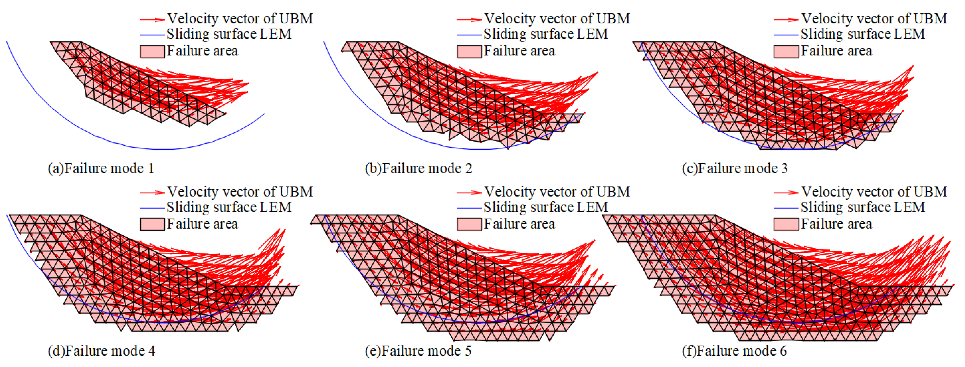
- When the randomness of the groundwater level and soil shear strength parameters are considered comprehensively, the traditional LEM will ignore multiple failure modes and may miscalculate the slope failure risk. However, all failure modes can be acquired with the UBM for seeking the minimum value of the KAVF. Thus, the result is more consistent with the real situation. In addition, the traditional LEM only judges the slope stability by the safety factor, which only reflects the degree of the IPF. The EFP is used to calculate the EFR of the slope, which cannot only reflect the degree of the IFP but, also, the slope failure risk can be accurately acquired. It should be noted that this calculation method can greatly reduce the calculation cost.
- (2)
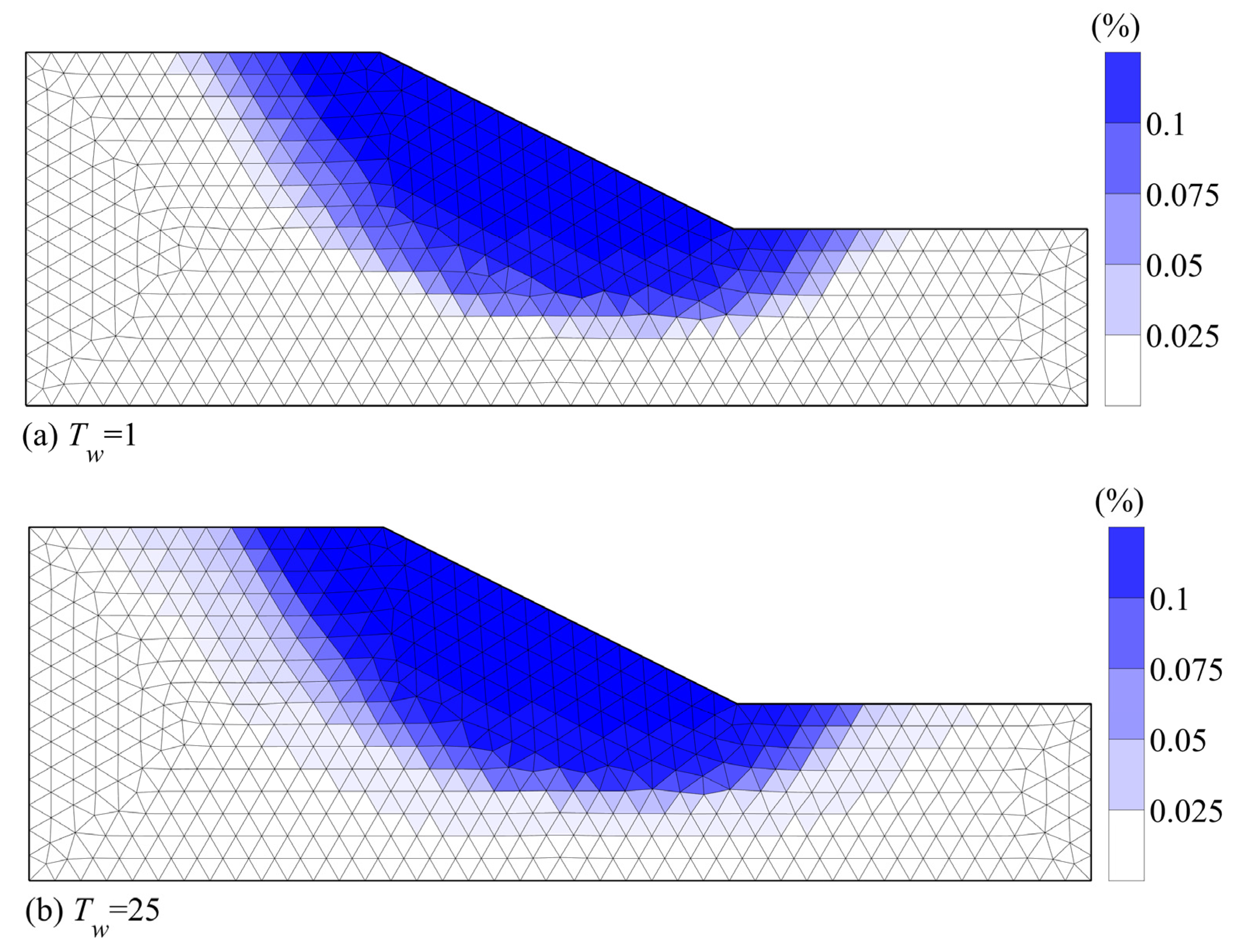
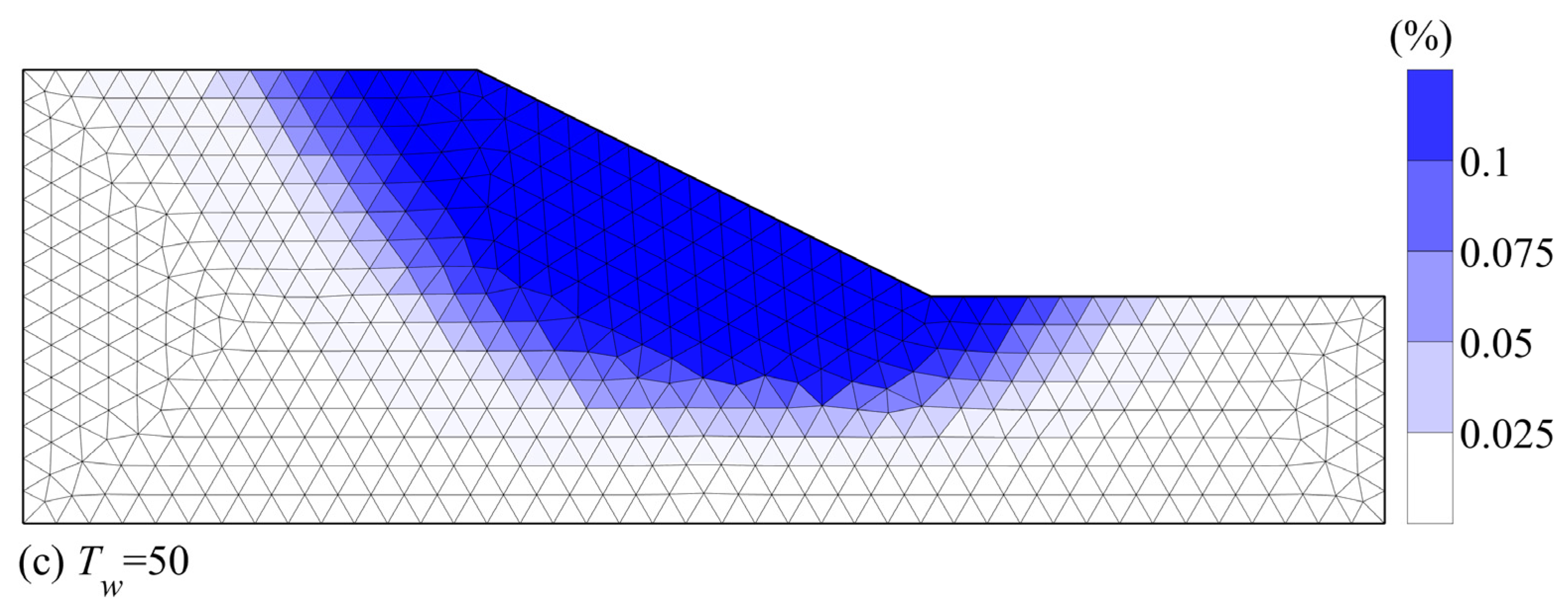
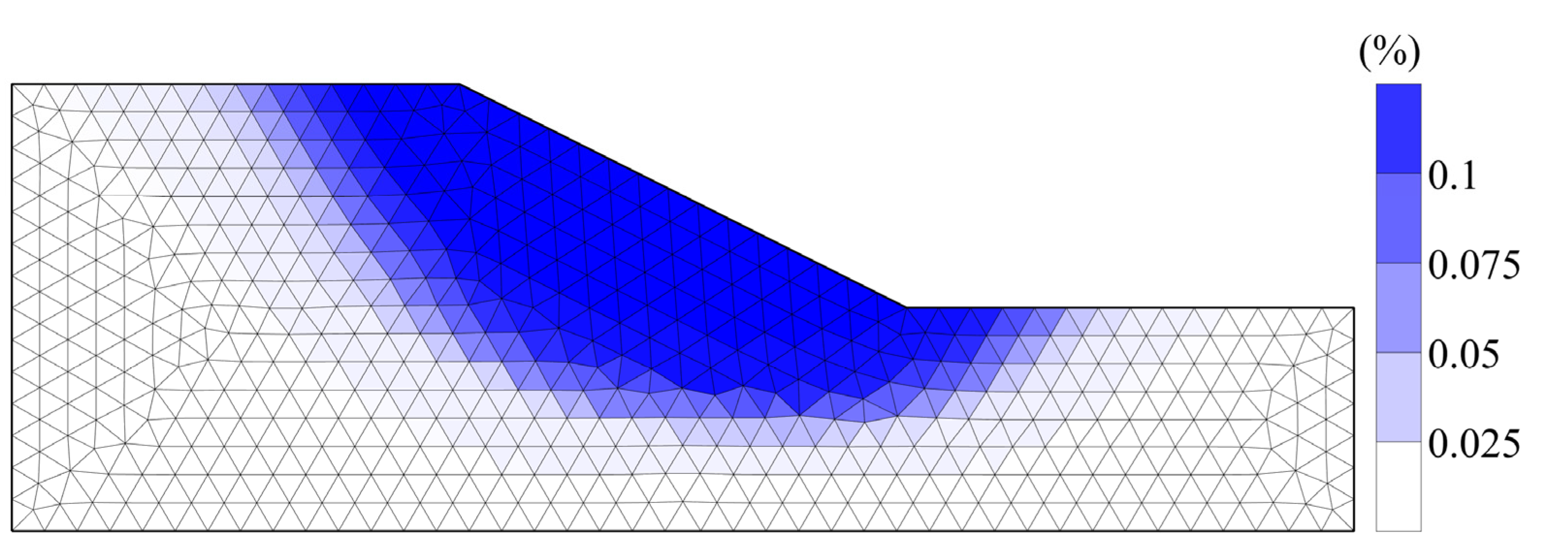
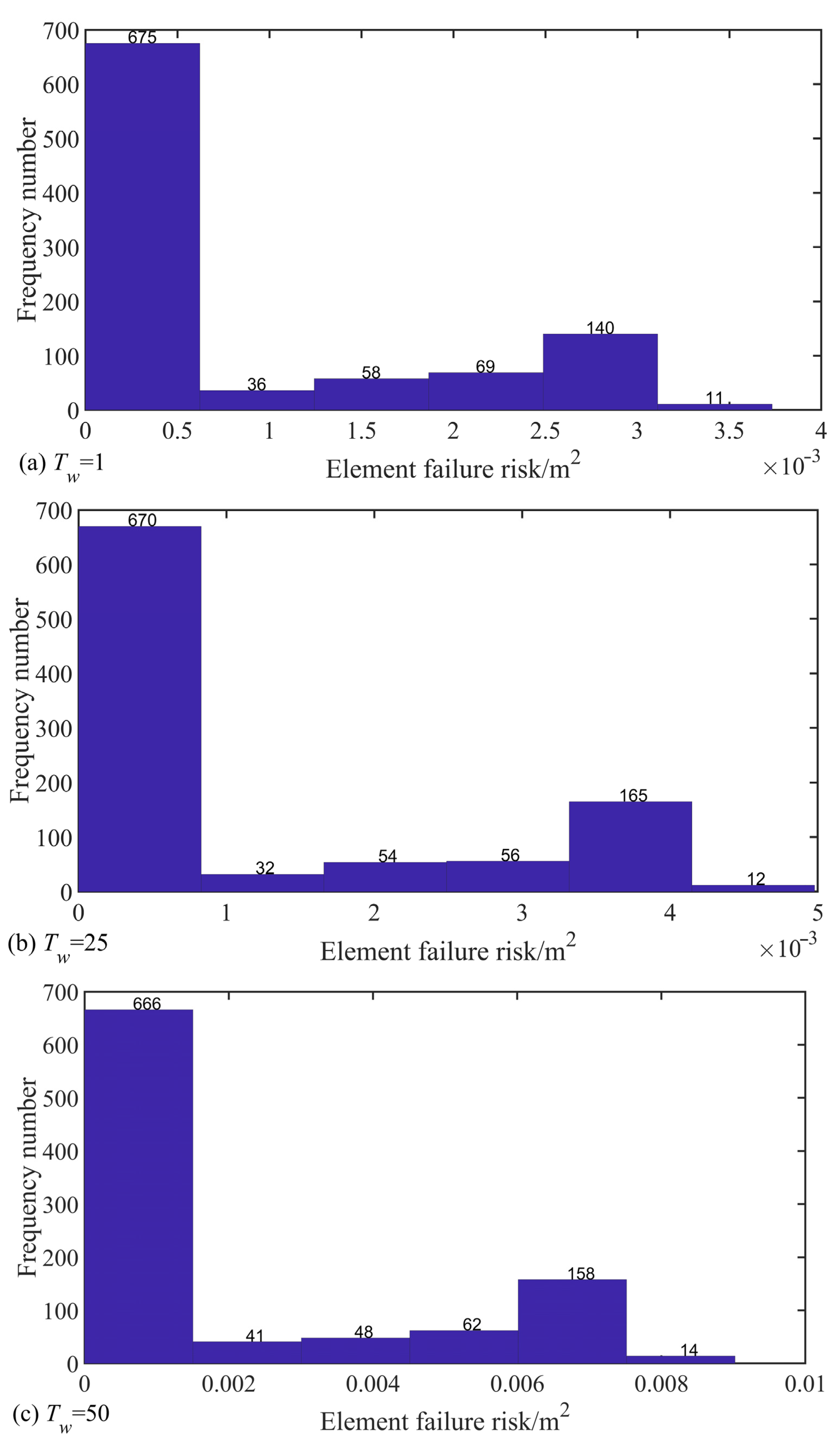
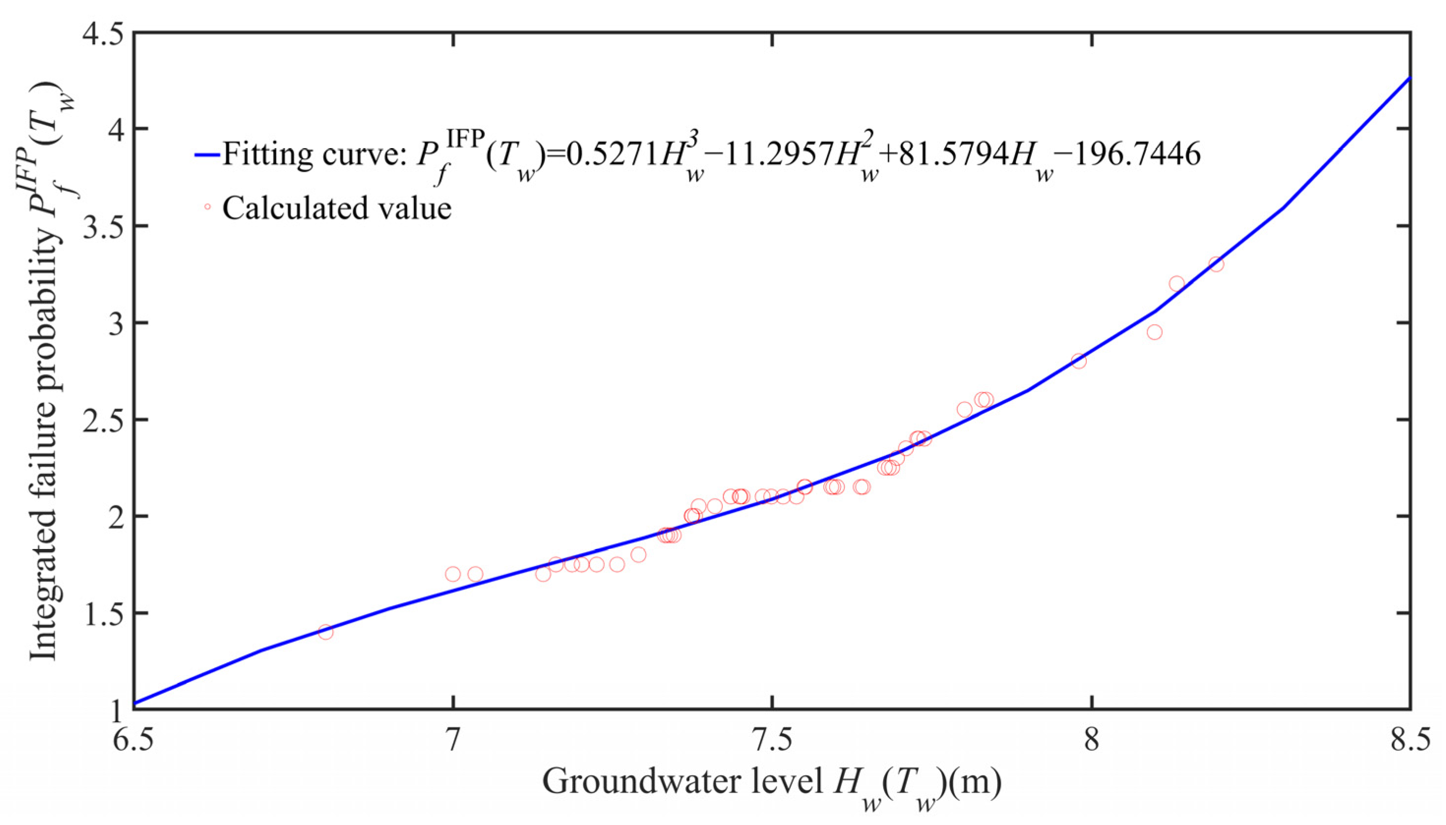
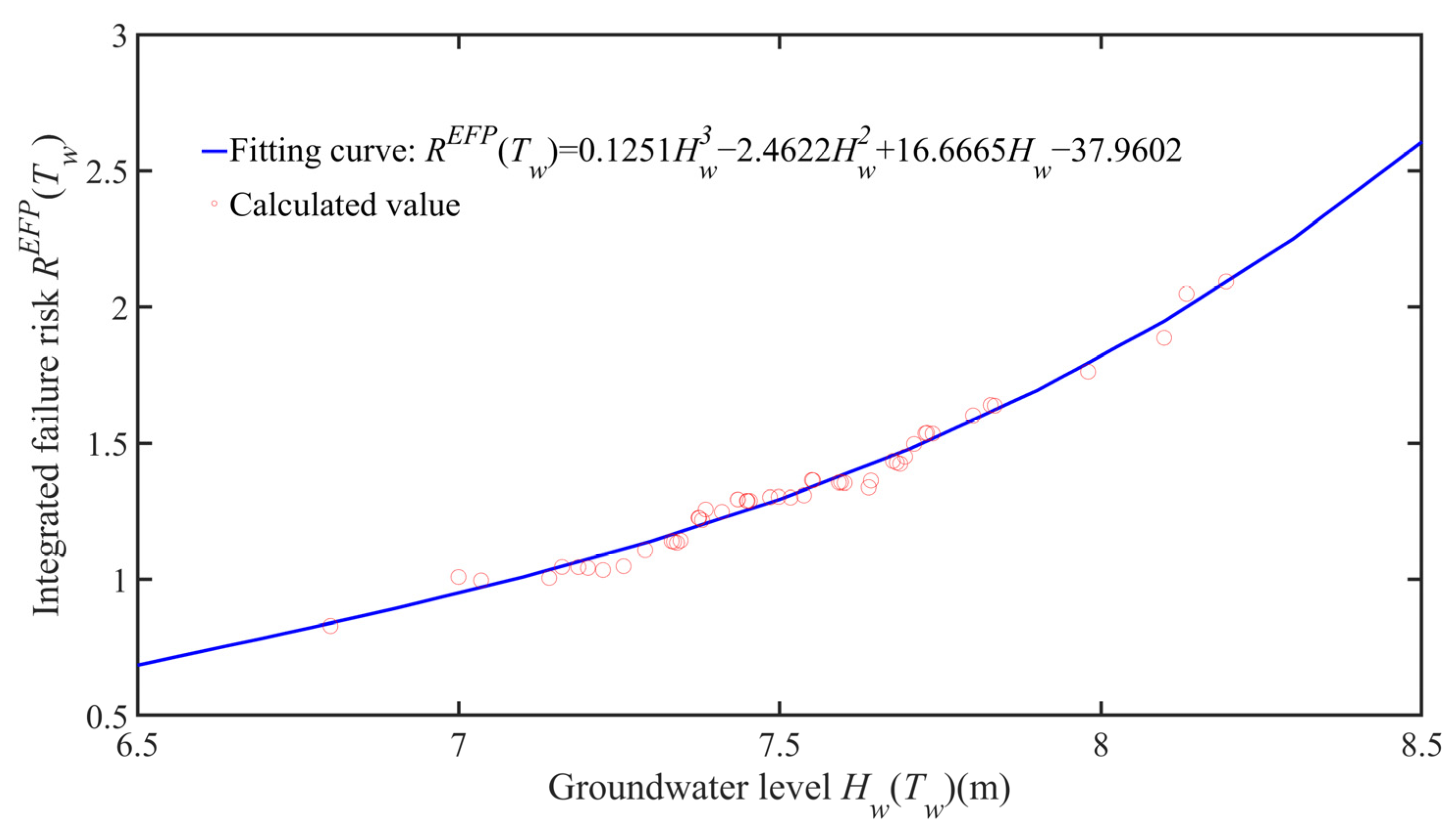
- The IFP and EFR of the slope are increasing from 1.40% to 3.30% and 0.829 m2 to 2.094 m2 with the rise of the groundwater level, respectively. Based on the EFP, the proposed method can accurately obtain the EFR of the slope under each groundwater level act by using the element’s location information and failure situation. This will provide engineers with realistic reference values for the slope reinforcement design to achieve sustainable development.
- (3)
- Groundwater level and earthquakes are two important causes of slope instability and failure. However, this study does not consider the impact of earthquakes on slope reliability. Therefore, relevant studies on seismic slope stability will be carried out in the future. In addition, according to the upper bound theory, the upper bound solution is inevitably greater than the true solution. Therefore, the failure probability will be underestimated when using the UBM for slope reliability analysis. To solve this problem, there is a necessity to study the slope reliability calculation method on the basis of the lower bound theory in future research work. The solution of slope failure probability with the UBM and LBM can be obtained at the same time, so the interval range of the real failure probability can be accurately judged, and the reliability index of the slope can be quantified more accurately.
Author Contributions
Funding
Institutional Review Board Statement
Informed Consent Statement
Data Availability Statement
Conflicts of Interest
References
- Dai, F.; Lee, C.; Ngai, Y. Landslide risk assessment and management: An overview. Eng. Geol. 2002, 64, 65–87. [Google Scholar] [CrossRef]
- Li, D.-Q.; Yang, Z.-Y.; Cao, Z.-J.; Zhang, L.-M. Area failure probability method for slope system failure risk assessment. Comput. Geotech. 2018, 107, 36–44. [Google Scholar] [CrossRef]
- Liu, X.; Li, D.-Q.; Cao, Z.-J.; Wang, Y. Adaptive Monte Carlo simulation method for system reliability analysis of slope stability based on limit equilibrium methods. Eng. Geol. 2020, 264, 105384. [Google Scholar] [CrossRef]
- Wang, L.; Wu, C.; Li, Y.; Liu, H.; Zhang, W.; Chen, X. Probabilistic Risk Assessment of unsaturated Slope Failure Considering Spatial Variability of Hydraulic Parameters. KSCE J. Civ. Eng. 2019, 23, 5032–5040. [Google Scholar] [CrossRef]
- Malkawi, A.I.H.; Hassan, W.F.; Abdulla, F.A. Uncertainty and reliability analysis applied to slope stability. Struct. Saf. 2000, 22, 161–187. [Google Scholar] [CrossRef]
- Zhao, H.-B. Slope reliability analysis using a support vector machine. Comput. Geotech. 2008, 35, 459–467. [Google Scholar] [CrossRef]
- Ching, J.; Phoon, K.-K.; Hu, Y.-G. Efficient Evaluation of Reliability for Slopes with Circular Slip Surfaces Using Importance Sampling. J. Geotech. Geoenviro. Eng. 2009, 135, 768–777. [Google Scholar] [CrossRef]
- Tang, X.-S.; Li, D.-Q.; Chen, Y.-F.; Zhou, C.-B.; Zhang, L.-M. Improved knowledge-based clustered partitioning approach and its application to slope reliability analysis. Comput. Geotech. 2012, 45, 34–43. [Google Scholar] [CrossRef]
- Cho, S.E. First-order reliability analysis of slope considering multiple failure modes. Eng. Geol. 2013, 154, 98–105. [Google Scholar] [CrossRef]
- Ji, J.; Zhang, W.; Zhang, F.; Gao, Y.; Lü, Q. Reliability analysis on permanent displacement of earth slopes using the simplified Bishop method. Comput. Geotech. 2020, 117, 103286. [Google Scholar] [CrossRef]
- Wang, W.; Li, D.-Q.; Liu, Y.; Du, W. Influence of ground motion duration on the seismic performance of earth slopes based on numerical analysis. Soil Dyn. Earthq. Eng. 2021, 143, 106595. [Google Scholar] [CrossRef]
- Griffiths, D.V.; Huang, J.; Fenton, G.A. Influence of Spatial Variability on Slope Reliability Using 2-D Random Fields. J. Geotech. Geoenviron. Eng. 2009, 135, 1367–1378. [Google Scholar] [CrossRef]
- Shen, H.; Abbas, S.M. Rock slope reliability analysis based on distinct element method and random set theory. Int. J. Rock Mech. Min. Sci. 2013, 61, 15–22. [Google Scholar] [CrossRef]
- Li, D.-Q.; Jiang, S.-H.; Cao, Z.-J.; Zhou, W.; Zhou, C.-B.; Zhang, L.-M. A multiple response-surface method for slope reliability analysis considering spatial variability of soil properties. Eng. Geol. 2015, 187, 60–72. [Google Scholar] [CrossRef]
- Wang, M.-Y.; Liu, Y.; Ding, Y.-N.; Yi, B.-L. Probabilistic stability analyses of multi-stage soil slopes by bivariate random fields and finite element methods. Comput. Geotech. 2020, 122, 103529. [Google Scholar] [CrossRef]
- Dyson, A.P.; Tolooiyan, A. Comparative Approaches to Probabilistic Finite Element Methods for Slope Stability Analysis. Simul. Model. Pract. Theory 2020, 100, 102061. [Google Scholar] [CrossRef]
- Lysmer, J. Limit Analysis of Plane Problems in Soil Mechanics. J. Soil Mech. Found. Div. 1970, 96, 1311–1334. [Google Scholar] [CrossRef]
- Li, Z.; Chen, Y.; Guo, Y.; Zhang, X.; Du, S. Element Failure Probability of Soil Slope under Consideration of Random Groundwater Level. Int. J. Géoméch. 2021, 21, 04021108. [Google Scholar] [CrossRef]
- Sloan, S.W. Lower bound limit analysis using finite elements and linear programming. Int. J. Numer. Anal. Methods Géoméch. 1988, 12, 61–77. [Google Scholar] [CrossRef]
- Sloan, S.; Kleeman, P. Upper bound limit analysis using discontinuous velocity fields. Comput. Methods Appl. Mech. Eng. 1995, 127, 293–314. [Google Scholar] [CrossRef]
- Li, Z.; Hu, Z.; Zhang, X.; Du, S.; Guo, Y.; Wang, J. Reliability analysis of a rock slope based on plastic limit analysis theory with multiple failure modes. Comput. Geotech. 2019, 110, 132–147. [Google Scholar] [CrossRef]
- Kim, J.; Salgado, R.; Yu, H.S. Limit Analysis of Soil Slopes Subjected to Pore-Water Pressures. J. Geotech. Geoenviron. Eng. 1999, 125, 49–58. [Google Scholar] [CrossRef]
- Li, Z.; Zhou, Y.; Guo, Y. Upper-Bound Analysis for Stone Retaining Wall Slope Based on Mixed Numerical Discretization. Int. J. Géoméch. 2018, 18, 04018122. [Google Scholar] [CrossRef]
- Liu, W.; Xu, H.; Sui, S.; Li, Z.; Zhang, X.; Peng, P. Lower Bound Limit Analysis of Non-Persistent Jointed Rock Masses Using Mixed Numerical Discretization. Appl. Sci. 2022, 12, 12945. [Google Scholar] [CrossRef]
- Chen, Z.H.; Lei, J.; Huang, J.H.; Cheng, X.H.; Zhang, Z.C. Finite element limit analysis of slope stability considering spatial variability of soil strengths. Chin. J. Geotech. Eng. 2018, 40, 985–993. [Google Scholar] [CrossRef]
- Peng, P.; Li, Z.; Zhang, X.Y.; Shen, L.F.; Xu, Y. Research on element failure probability and failure mode of soil slope. Eng. Mech. 2022, 39, 1–15. [Google Scholar] [CrossRef]
- Silva, F.; Lambe, T.W.; Marr, W.A. Probability and Risk of Slope Failure. J. Geotech. Geoenviron. Eng. 2008, 134, 1691–1699. [Google Scholar] [CrossRef]
- Cassidy, M.J.; Uzielli, M.; Lacasse, S. Probability risk assessment of landslides: A case study at Finneidfjord. Can. Geotech. J. 2008, 45, 1250–1267. [Google Scholar] [CrossRef]
- Zhang, X.Y.; Zhang, L.X.; Li, Z. Reliability analysis of soil slope based on upper bound method of limit analysis. Rock Soil Mech. 2018, 39, 1840–1850. [Google Scholar] [CrossRef]
- Zuo, Z.; Zhang, L.; Cheng, Y.; Wang, J.; He, Y. Probabilistic back analysis of unsaturated soil seepage parameters based on Markov chain Monte Carlo method. Rock Soil Mech. 2013, 34, 2393–2400. [Google Scholar]
- Wang, X.; Xia, X.; Zhang, X.; Gu, X.; Zhang, Q. Probabilistic Risk Assessment of Soil Slope Stability Subjected to Water Drawdown by Finite Element Limit Analysis. Appl. Sci. 2022, 12, 10282. [Google Scholar] [CrossRef]
- Cho, S.E.; Park, H.C. Effect of spatial variability of cross-correlated soil properties on bearing capacity of strip footing. Int. J. Numer. Anal. Methods Géoméch. 2010, 34, 1–26. [Google Scholar] [CrossRef]
- Shadabfar, M.; Huang, H.; Kordestani, H.; Muho, E.V. Reliability Analysis of Slope Stability Considering Uncertainty in Water Table Level. ASCE-ASME J. Risk Uncertain. Eng. Syst. Part A Civ. Eng. 2020, 6, 04020025. [Google Scholar] [CrossRef]
- Li, K.S.; Lumb, P. Probabilistic design of slopes. Can. Geotech. J. 1987, 24, 520–535. [Google Scholar] [CrossRef]
- Li, D.Q.; Jiang, S.H.; Zhou, C.B.; Phoon, K.K. Reliability analysis of slopes considering spatial variability of soil parameters using non-intrusive stochastic finite element method. Chin. J. Geotech. Eng. 2013, 35, 1413–1421. [Google Scholar]
- Zhou, J.; Qin, C. Stability analysis of unsaturated soil slopes under reservoir drawdown and rainfall conditions: Steady and transient state analysis. Comput. Geotech. 2022, 142, 104541. [Google Scholar] [CrossRef]
- Huang, J.; Lyamin, A.; Griffiths, D.V.; Krabbenhoft, K.; Sloan, S. Quantitative risk assessment of landslide by limit analysis and random fields. Comput. Geotech. 2013, 53, 60–67. [Google Scholar] [CrossRef]


| Shear Parameter | Mean | Correlation of Variation | Distribution Type | Fluctuation Range | Correlation Coefficient |
|---|---|---|---|---|---|
| c(kPa) | 10 | 0.3 | Lognormal | Lh = 40 m Lv = 4 m | ρc,φ = −0.5 |
| φ(°) | 30 | 0.2 | Lognormal |
| Groundwater Level | Method | Mean | Standard Deviation | Failure Probability (%) |
|---|---|---|---|---|
| Tw = 1 | UBM | 1.2956 | 0.1420 | 1.40 |
| LEM | 1.2923 | 0.1488 | 1.90 | |
| Tw = 25 | UBM | 1.2678 | 0.1394 | 2.10 |
| LEM | 1.2622 | 0.1461 | 2.70 | |
| Tw = 50 | UBM | 1.2357 | 0.1365 | 3.30 |
| LEM | 1.2310 | 0.1432 | 4.65 |
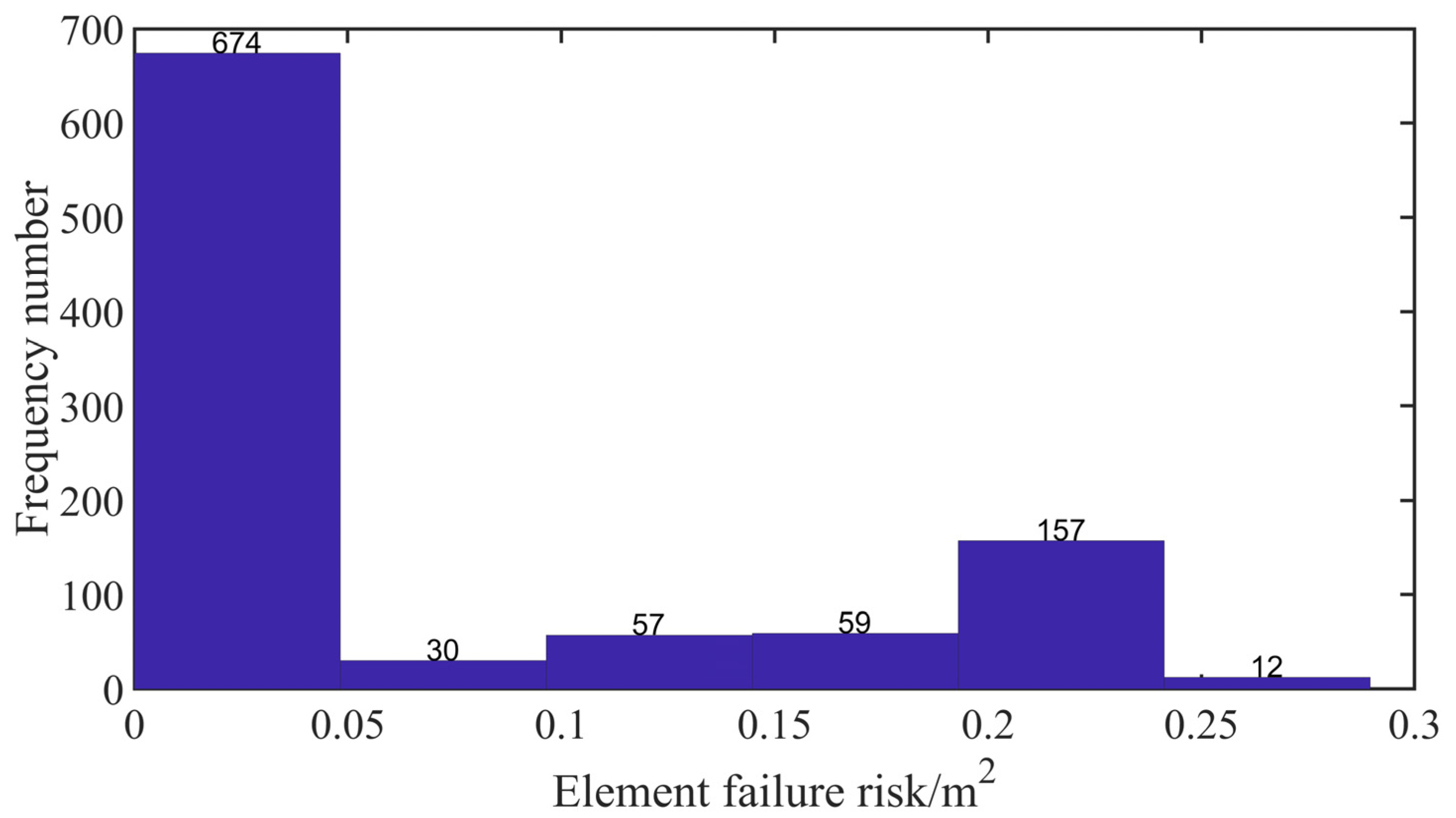
| Failure Mode | Failure Area (m2) | Failure Times | Failure Probability (%) | Failure Risk (m2) |
|---|---|---|---|---|
| Mode 1 | 28.68–43.70 | 246 | 0.246 | 0.097 |
| Mode 2 | 43.81–58.91 | 751 | 0.751 | 0.384 |
| Mode 3 | 58.91–73.96 | 768 | 0.768 | 0.508 |
| Mode 4 | 74.21–89.04 | 221 | 0.221 | 0.180 |
| Mode 5 | 89.17–103.70 | 88 | 0.088 | 0.081 |
| Mode 6 | 106.71–119.38 | 72 | 0.072 | 0.081 |
| Sum | / | 2146 | 2.146 | 1.332 |
| Groundwater Level | Failure Mode | Failure Times | Failure Probability (%) | Failure Risk (m2) |
|---|---|---|---|---|
| Tw = 1 | Mode 1 | 3 | 0.15 | 0.057 |
| Mode 2 | 13 | 0.65 | 0.334 | |
| Mode 3 | 10 | 0.50 | 0.342 | |
| Mode 4 | 1 | 0.05 | 0.038 | |
| Mode 6 | 1 | 0.05 | 0.057 | |
| Tw = 25 | Mode 1 | 5 | 0.25 | 0.096 |
| Mode 2 | 14 | 0.70 | 0.366 | |
| Mode 3 | 16 | 0.80 | 0.528 | |
| Mode 4 | 5 | 0.25 | 0.210 | |
| Mode 5 | 1 | 0.05 | 0.045 | |
| Mode 6 | 1 | 0.05 | 0.056 | |
| Tw = 50 | Mode 1 | 8 | 0.40 | 0.160 |
| Mode 2 | 19 | 0.95 | 0.490 | |
| Mode 3 | 24 | 1.20 | 0.793 | |
| Mode 4 | 11 | 0.55 | 0.445 | |
| Mode 5 | 2 | 0.10 | 0.091 | |
| Mode 6 | 2 | 0.10 | 0.115 |
| Method | LEM with Equation (12) | UBM with Equation (14) | UBM with Equation (22) | |
|---|---|---|---|---|
| Groundwater | ||||
| Tw = 1 | 1.121 | 0.829 | 0.829 | |
| Tw = 25 | 1.593 | 1.302 | 1.302 | |
| Tw = 50 | 2.325 | 2.094 | 2.094 | |
Disclaimer/Publisher’s Note: The statements, opinions and data contained in all publications are solely those of the individual author(s) and contributor(s) and not of MDPI and/or the editor(s). MDPI and/or the editor(s) disclaim responsibility for any injury to people or property resulting from any ideas, methods, instructions or products referred to in the content. |
© 2023 by the authors. Licensee MDPI, Basel, Switzerland. This article is an open access article distributed under the terms and conditions of the Creative Commons Attribution (CC BY) license (https://creativecommons.org/licenses/by/4.0/).
Share and Cite
Peng, P.; Li, Z.; Zhang, X.; Liu, W.; Sui, S.; Xu, H. Slope Failure Risk Assessment Considering Both the Randomness of Groundwater Level and Soil Shear Strength Parameters. Sustainability 2023, 15, 7464. https://doi.org/10.3390/su15097464
Peng P, Li Z, Zhang X, Liu W, Sui S, Xu H. Slope Failure Risk Assessment Considering Both the Randomness of Groundwater Level and Soil Shear Strength Parameters. Sustainability. 2023; 15(9):7464. https://doi.org/10.3390/su15097464
Chicago/Turabian StylePeng, Pu, Ze Li, Xiaoyan Zhang, Wenlian Liu, Sugang Sui, and Hanhua Xu. 2023. "Slope Failure Risk Assessment Considering Both the Randomness of Groundwater Level and Soil Shear Strength Parameters" Sustainability 15, no. 9: 7464. https://doi.org/10.3390/su15097464