1. Introduction
Wind energy, both onshore and offshore, grows at a high rate driven by global decarbonization policies [
1]. This has accelerated the evolution of turbines [
2] and the need for additional research and development to meet market pressure [
3,
4]. In general, Computational Fluid Dynamic (CFD) simulations are commonly used in wind turbine modeling of high precision, mainly in the prospecting of power and energy density [
5]. However, some barriers arise when working with CFD techniques, such as the high investment in computational machines, the high computational burden, and the high level of difficulty in parameterizing and creating the shapes of the models. Due to these barriers, integral methods such as BEMT have been researched with the intention of working with less complex and fast-resolution simulations compared to CFD. The BEMT is an integral method capable of accurately predicting wind turbine performance [
6,
7].
Despite the fact that the classical BEMT is consolidated, considering the correction methods of Prandtl and Glauert [
8], more is needed to analyze and predict the performance of turbines in some specific conditions. In situations where the angle of attack oversteps the stall, the BEMT has considerable errors in the calculation of the thrust and torque forces along the blades [
8]. Therefore, mathematical correction models are needed and must be capable of equating the performance of the turbines in these situations.
Some of these mathematical models can be found in the state of the art presented in [
9], in which the aerodynamic performance of real onshore wind turbines is evaluated and discussed. The analysis presented in [
9], unlike the one proposed in this article, considered ideal flow conditions for wind turbine research. Even so, the state of the art presented and discussed in that article, and the model used to predict output power generation, contribute to studies of turbine performance prediction. The work described in [
10] predicted wind turbine power generation using a forecasting method. Machine learning-based modeling is proposed to predict the wind turbine power output. The methodology applied in [
10] is based on the measurement of physical variables such as wind speed and shaft rotational speed. This approach is interesting to analyze the performance of turbines from data acquisition, from a database, or in a real dynamic way since the mathematical model of the turbine power train is not necessary. In [
11], diffuser-augmented wind turbine technologies are investigated according to developments in the literature. The effect of the diffuser on power generation is ascertained based on experimental and numerical studies. Improvements in performance have been noticed among the reviewed studies.
Several methods derived from the BEMT are proposed for the performance analysis of wind turbines [
12,
13,
14]. In these methods, the authors implemented functions for complementary corrections focusing on the calculations of at least one of the following approaches: tip losses, high values of the axial induction factor, and high values of angle of attack in post-stall conditions. Some of these authors generally take into account only one of these complementary correction functions. They used the study of a single turbine as validation [
15], which can restrict the application, especially when empirical methods are proposed. Similar to [
16,
17], the work in [
18] presents research that addresses the direct calculation of tip loss, which can be solved in three different ways. Two of them are more accurate than the Prandtl method and have simple and faster implementation. They are appropriate and good for the blade element calculation of turbine performance but only address one type of correction method of BEMT. In [
19], a study on different correction methods is performed, but the analyses are limited to a single 100 kW turbine. Therefore, these methods are not tested for different turbine sizes regardless of the nominal output power range. According to [
20], small turbines differ significantly from medium and large ones in rotor design and manufacture. The main challenges for small ones are low operational Reynolds number (
), as small rotors usually operate at low wind speed, and the structural requirements of more rapidly rotating turbines. Moreover, most small turbines use ‘‘free yaw’’ whereby a tail fin, rather than an automatized yaw drive as on larger rotors, is used to align the turbine with the wind direction. It is worth noting that this work does not cover yaw behavior and associated issues of tail fin design and aerodynamic over-speed protection.
In this article, a study of a single, simple, and quick approach to estimating the power performance of any size turbine is employed. A comparative analysis of the simulated results with experimental data from real turbines is performed to validate the implemented approach.
Table 1 shows the data of small, medium, and large-sized turbines simulated. These data are obtained from published works in technical reports. The turbines correspond to one of 1.9 kW [
20] and four others of NASA MOD-X series turbines that are: 100 kW [
21,
22,
23], 2.5 MW [
24,
25,
26], and 7.3 MW [
27,
28,
29]. For the small turbine of 1.9 kW, a two-bladed and 3 m diameter turbine tested by Anderson et al. [
30] is used. Lift and drag coefficients for the airfoil NACA4412 for a Reynolds number range
is considered in the simulations. For the medium turbine of 100 kW, a two-bladed 38 m diameter rotor is employed. Lift and drag coefficients for the airfoil NACA23012 for a Reynolds number range
is taken into account. For the large turbine of 2.5 MW, a two-bladed 91.44 m diameter turbine is used. Lift and drag coefficients for the airfoil NACA23012 for a Reynolds number range
is applied. For the large turbine of 7.3 MW, a two-bladed 121.92 m diameter turbine is used. Lift and drag coefficients for the airfoil NACA64015 for a Reynolds number range
is considered in the simulations. Unfortunately, airfoil data from experimental studies in wind tunnels are not easily available in the literature, even more when these data are desired for different Reynold numbers [
31]. Based on this context, the airfoil data for the NASA turbines are obtained from [
32], so they could be simulated. Except for the small turbine, each of the others uses the same class of airfoils along the blade. Where the airfoil thickness increases from the tip to the hub blade. The blade root area provides mechanical resistance to support the distribution of forces along the rotor.
Approaches based on BEMT are easy to implement, with low computational burden and good accuracy in calculating turbine performance [
7]. They can be implemented and executed in largely available software. Additionally, they can run on the Simulink Platform and integrate power system simulations that can be solved in a few minutes. CFD simulation methods use numerical techniques to solve problems related to fluid dynamics [
33]. These methods are based on the discretization of a domain with so many degrees of freedom from a finite system, using different mathematical equations [
34]. Finite Volume Methods, for example, are based on the discretization of the differential form of the governing equations (continuity equations) and work by approximating the derivative through expansions of mathematical series [
35]. CFD software is indeed a great tool to analyze wind turbine performance, [
34,
36]. However, they can take hours, days, or even weeks to obtain a result.
In this context, the proposed study is developed from the classical BEMT with the addition of complementary corrections for tip and root losses, for high values of the axial induction factor, and for high angle of attack to better represent the performance of the turbines. The research is based on a study of the mathematical model involved in the BEMT. The complementary correction methods were exhaustively researched in the literature. The corrections are included in the BEMT in order to analyze the best performance for simulating small, medium, and large turbines. The results combine three kinds of correction, and the best ones are presented and discussed. The main contribution of the work is to propose a stable BEMT numerical algorithm through the assessment of the combination of the correction methods available in the literature, classical, and modern ones. The algorithm ensures applicability for small, medium, and large-sized wind turbines, as well as being fast and easy to implement in any computer and simpler than CFD, which is usually time-consuming and complex to operate [
37]. Another important characteristic of the proposed algorithm is the extensibility of turbines with diffusers, which can be achieved through the inclusion of the direct calculation of tip loss as described by Wood et al. [
18].
The remainder of this article is organized as follows. In
Section 2, the summarized modeling of the classical BEMT method and the justification for the need for complementary correction methods are presented. It also discusses the types of complementary corrections, for which different methods proposed in the literature are shown. In addition, the modified and implemented BEMT method to perform the wind turbine simulations is presented in a flowchart form.
Section 3 presents the results, discussing the accuracy obtained from the simulations of the implemented BEMT algorithm. Finally,
Section 4 states the conclusions about the approach that best calculates turbine performance, regardless of the power range.
2. Description of Methods
Simple mathematical modeling based on Betz’s research can be used to determine the output power of an ideal turbine rotor. This modeling is based on a linear momentum theory. The analysis of this theory considers a control volume whose boundaries are the surface of a stream tube and two cross-sections of the stream tube. A uniform actuator disc represents the wind turbine and creates a discontinuity of pressure through it [
38]. This analysis considers (i) steady-state fluid flow; (ii) homogenous and incompressible fluid; (iii) insignificant frictional drag (can be approximated to zero); (iv) infinite number of blades; (v) uniform thrust over the disc or rotor area; (vi) non–rotating wake; (vii) the static pressure far upstream and far downstream of the rotor is equal to the undisturbed; and (viii) ambient static pressure. Furthermore, this model is not valid for an axial induction factor higher than 0.4, as it complicates the flow patterns, not representing the thrust coefficient, which can be higher than 2.0 [
8,
38]. Therefore, these high values of the axial induction factor are corrected through complementary correction methods that are presented and discussed in the following sections.
In the case of a wind turbine, the flow behind the rotor rotates in the opposite direction to the shaft in reaction to the torque exerted by the flow on the rotor blades. The generation of rotational kinetic energy in the wake results in less energy extraction by the turbine than would be expected without wake rotation. If the wake rotation becomes high, extra suction will be created behind the turbine since a radial pressure gradient is needed to maintain the curved streamlines. Then, the pressure becomes lower as the radial distance becomes smaller. This lower pressure at the center behind the disc creates an extra mass flow through the disc, which needs to be accounted for when using the momentum equation, where the pressure is assumed constant [
8].
2.1. Effects Related to Loss of Performance
Three conditions lead to a decrease in turbine efficiency and should be considered in the analysis [
8,
39]: (i) the finite number of blades and related tip losses [
40]; (ii) rotation of the wake in the region behind the rotor; and (iii) aerodynamic drag. Whenever the wake rotation is accounted for in the analysis, the induced velocity at the rotor consists of the axial component and of the component in the rotor plane. As a result, (i) the power coefficient curve increases exponentially from zero to the maximum theoretical limit, 0.59, as a function of the increase in tip speed ratio; (ii) the axial induction factor increases exponentially from an initial value to the maximum theoretical limit, 1/3, along the rotor radius from the hub; and (iii) the rotation induction factor decreases exponentially from an initial high value to the minimum along the rotor radius from the hub.
Concerning wake rotation, typical for BEMT analysis, any velocity in the radial direction is ignored, and only rotational velocity is included. In this work, the same condition is considered, and no attempt is made to include radial effects of the wake rotation in the blade element calculations. Additionally, it is important to emphasize that for airfoil behavior the flow along the radius of the rotor can remain at angles of attack of the stall region. In the literature, it is still not clear what causes the stall. Possibly, the stall can be influenced by Coriolis and centrifugal forces, as pointed out by [
20,
41]. According to [
20], stall supposedly depends on a parameter that does not measure the centrifugal and Coriolis forces because it does not contain the turbine’s rotational speed. It mostly occurs near the hub, so it is probable that solidity, which is typically higher near the hub and delays separation, is at least in part responsible. In other words, the cascade effect is relevant to account for the stall, especially for multibladed turbines. It is important to highlight that the stall does not significantly influence turbines with optimized performance. In this work, the stall phenomenon is corrected using the model presented by Viterna and Corrigan [
42], as detailed later.
2.2. Blade Element Momentum Theory
The BEMT method and its derivations are discussed in this work. The main approach is the combination of two theories: (i) the axial momentum, and (ii) the blade element. In these analyses, a free, unidirectional, and incompressible flow is considered to derivate mathematical equations [
41,
42]. This method analyzes the transformation of kinetic energy transported by the fluid into mechanical energy through the axis of the turbine due to the interactions of the fluid with the rotor blades. It is an integrative model, calculated by semi-empirical data of aerodynamic forces that act on the blade based on sections of airfoils. These forces are calculated using the lift and drag coefficients, which can be acquired from a two-dimensional flow model or from experimental data.
Combining these unidimensional and two-dimensional procedures is based on equations of thrust and torque forces from each theory [
41,
42]. According to the axial moment theory, the elemental thrust (defined in this theory as
) and elemental torque (
) equations are presented in Equations (1) and (2), respectively.
where
is the velocity of the free upstream fluid,
is the density of the fluid,
is the local radius of the ideal turbine,
is the rotational speed of the rotor,
is the axil induction factor, and
is the rotational induction factor.
With respect to the blade element theory, the elemental thrust (defined in this theory as
) and elemental torque (
) are expressed in Equations (3) and (4), respectively [
41,
42].
where
is the local solidity,
is the flow angle formed between the plane of rotation and the flow relative velocity,
and
are the coefficients of normal and tangential forces, respectively.
The elemental mechanical output power (
) and the power coefficient (
) can be calculated using Equations (5) and (6), respectively. The mechanical power output (
) can be calculated by integrating Equation (5) as a function of the radial position [
41,
42].
where
is the tip radius of the rotor.
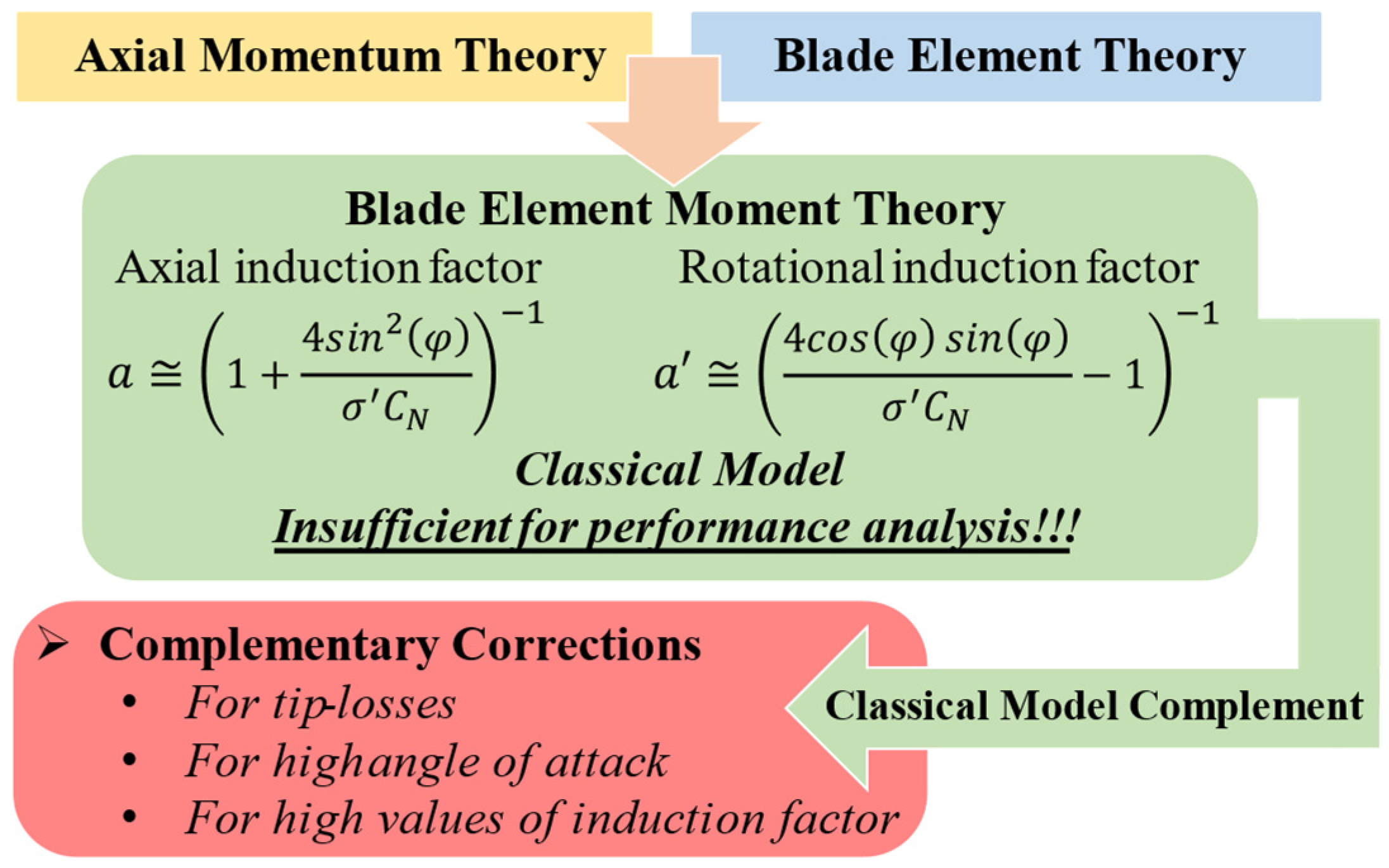
Figure 1 illustrates the combination of these two theories, from which the classical BEMT is built. The specifications of this method can be checked in [
19]. Additionally, the necessary types of corrections to complement this theory are shown, so that the simulation results can reach satisfactory outcomes for wind turbines. The following sections will present and review these corrections proposed in the literature.
2.3. Description of Complementary Methods to Classical BEMT
Although the BEMT is consolidated, the derivation of thrust, torque, and power equations do not correctly express turbine performance. Therefore, complementary corrections are needed.
2.3.1. Tip and Hub Losses
Classical BEMT does not consider tip and hub losses, but they are important for analyzing the turbine’s performance since they directly interfere with torque calculation. The classic approach assumes that there is an appropriate number of blades for all fluid particles passing through the rotor to interact with the blades. However, with a minor number of blades (modern turbines are built with three blades), some particles of the fluid will interact with them. However, most will pass between the blades and the loss of momentum by a particle will depend on its nearness to a blade [
41]. The tip loss on the blade is a consequence of the influence of the vortices that arise along the blade, which reduces the circulation, and consequently, the aerodynamic efficiency. The axial induced velocity will, therefore, vary around the blade. This directly influences the torque to which the blade is submitted. In practical terms, the loss factor is always less than unity impacting around 5 to 10% in predictive calculations of the power performance curve [
20].
The extension of the BEMT, to take into account a finite number of blades, usually needs a tip loss factor (F). Okulov et al. [
43] extended the Betz limit to a finite number of blades using the Prandtl method [
44]. Therefore, the
of Prandtl is defined as the ratio between the actual limited circulation and that of a rotor with an infinite number of blades.
The blade element calculations made with the Prandtl model show good accuracy with the experimental data [
45,
46] for a high tip speed ratio. Wood et al. [
18] showed that blade element calculation is imprecise for a very low tip speed ratio (smaller than 1). Nevertheless, all simulations in this article are performed for tip speed ratio superior unity.
In general, the mathematical models for correcting losses along the blade consider only the tip region. However, even though the contribution to the power and thrust from the hub region is small [
47]. The losses due to circulation at the blade root need to be physically consistent with the classical vortex theory, e.g., lifting line analyses of horizontal-axis turbines demonstrate that helicoidal vorticity shed from the blades goes to zero at the blade root for a bare turbine, as further described in [
48]. According to [
41], at the root of a turbine blade without a diffuser, the circulation must fall to zero as it does at the blade tip. This tendency can be observed in [
49], which used CFD simulation to analyze blade tip flow past a 95 kW Tellus rotor equipped with LM8.2 blades. Then, it is presumable that a similar process occurs in both regions, tip and root. At the blade tip, the impact of losses is considerable compared to the root, directly influencing turbine power by 5–10%, as in [
18,
50]. Therefore, the Prandtl correction factor is calculated for the tip (
) and root regions (
) of the blade as shown in Equations (7) and (8), [
8,
42].
where
is the rotor radius,
is the root radius of the rotor, and
is the number of blades.
The total factor loss (
) resultant considers the losses at the blade’s tip and root, as shown in Equation (9). Some blades’ shape is uniform up to the hub. In this condition, the losses in the root region can be ignored [
8,
38,
41,
42].
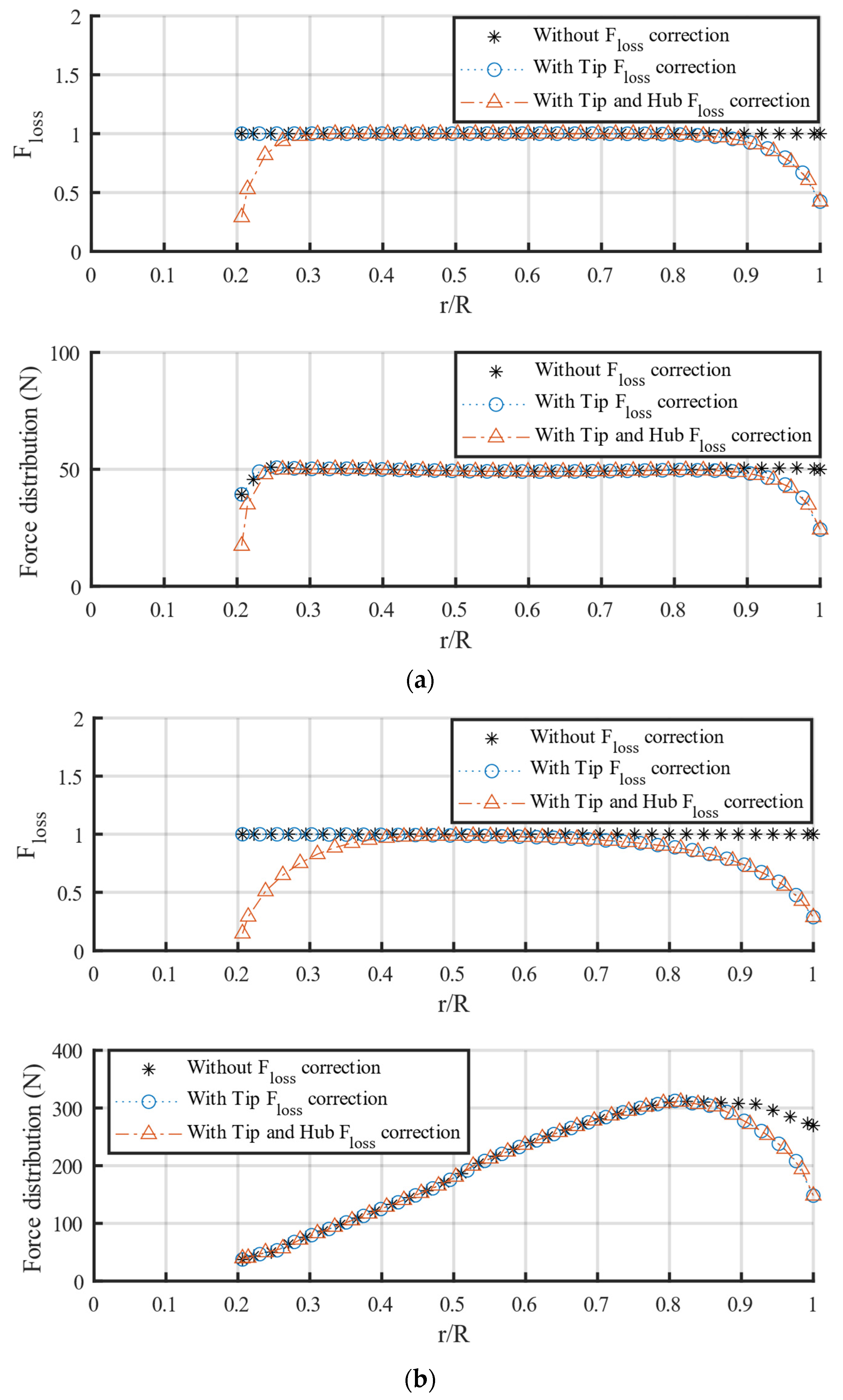
Figure 2a,b shows in the upper graphs that the losses due to vortices shedding affect
only the blade’s tip, leading to a reduction. When the correction is applied to both root (
) and tip (
),
reduces. Analyzing the bottom graph of
Figure 2a, which shows the force distribution curve along the rotor radius in the turbine starting condition, it is possible to observe that both root and tip corrections decrease, influencing the force distribution along the radial position, in ranges
and
. This becomes more evident at the turbine starting condition because the blade root has a significant torque contribution, as the angle of attack at very low rotational speed is much lower at the root than at the tip, affecting the torque. The bottom graph of
Figure 2b shows the force distribution curve along the blade. The turbine is under operating conditions close to nominal. It is possible to observe the influence of the tip correction rather than the root correction. This happens because, close to the nominal condition, the tip loss is by far the most significant contributor to turbine torque, as the lift-to-drag ratio is close to the optimum.
Prandtl proposed more expressions [
51] with Betz, which are named the Prandtl M1 given by Equation (10) and the Prandtl M2 given by Equation (11). In this model, Prandtl and Betz assumed a finite number of blades and considered the wake vortex theory. The difference between these methods is that, in Equation (10), the velocity component at the rotor plane (
) is calculated exactly by
, and in Equation (11) it is calculated approximately by
[
51].
where
is the tip speed ratio and
is local tip speed ratio.
Burton proposed a method [
38], shown in Equation (12), similar to that of Prandtl [
51], shown in Equation (10). The results obtained with these methods are overestimated for any power range of the turbines.
Among all the methods found in the literature to consider tip loss, the simplest empirical method is the Effective Radius [
42], which can be calculated by Equations (13) and (14). The vortices in the blade tip region significantly affect the rotor torque and thrust compared to the hub region. Based on this knowledge, tip loss can be accounted for by defining an effective rotor radius (
), which is about 3% smaller than the true tip radius (
) [
42].
Once the
is calculated, the equations of the induction factors must consider it. Those equations are shown in
Figure 1,
and
can be calculated by Equations (15) and (16) [
8,
38,
41,
42].
2.3.2. Correction Method Applied Simultaneously for the Tip Loss and Induction Factors
BEMT calculations with Prandtl tip loss present good accuracy at a high value of
, as seen in [
52]. However, it is shown in [
18] that it is inaccurate at very low
, and in the region close to the turbine axis, it does not represent
for values greater than unity. Moreover,
is found to be imprecise along the blade and has a significant error in the region close to the hub at any
.
Wood et al. [
18] proposed an alternative method using helical vortex theory, analyzing the nonlinear terms in equations of the streamtube with attention to angular and axial momentum. They found an accurate way of including these equations in BEMT calculations [
53]. From these works, the calculated results showed higher induced axial velocities in the tip and hub regions. Therefore, the trailing vorticity functions could be used in conditions where
cannot. For this method, the torque and thrust coefficients are calculated using Equations (17) and (18) [
53].
where
is the induction factor value at the blade,
is the rotational induction factor at the blade;
and
are the loss for axial and circumferential motion.
and
are calculated using Equations (19) and (20), and
and
are calculated using Equations (21) and (22) [
53].
where
and
are two intermediate functions similar to those implemented by Shen et al. [
47], and are defined by Equations (23) and (24).
The equation for
can be obtained by multiplying the
by
, where
is calculated using Equation (25) [
53].
where
is an auxiliary variable and it is calculated by (26).
where
is the pitch calculated using Equation (27) and
is the bound circulation of the blade element.
is calculated using Equation (28).
Similar to the other methods, the use of vortex theory does not account for high thrust and the need to correct Equation (17) in this region. By analogy, with equations of Shen et al. [
29], for
, Equations (29) and (30) are used.
2.3.3. Induction Factor Correction
The methods for the correction of the classical BEMT, for high values of the axial induction factor, generally, are based on relationships derived from the study conducted by Glauert [
8,
41,
42]. Glauert’s empirical relationship states that under turbulent wake conditions (
), the thrust coefficient (
increases up to 2.0 for
, [
38]. The BEMT fails for
and for this region the induction factor correction is particularly important. The correction proposed by Glauert [
38] is applied for
or
, as presented in Equations (31) and (32). Glauert fit a parabola to some data of rotors operating in a turbulent wake state to obtain these equations. This parabola agrees well with the classical momentum curve up to
a = 0.4. However, a numerical problem arises in the classical momentum equation when the loss correction factor [
54] is applied: a discontinuity appears between the theoretical curve and the correction method.
Peter Smith presents modeling for
[
23,
24], and it can be calculated using Equations (33)–(35). The development of this model is based on applications with low wind speeds where
is large.
where
and
are auxiliary variables.
Robert Wilson presents modeling for
[
55,
56], and it can be calculated using Equations (36) and (37). In low-thrust regions, the results can show considerable errors.
where
is an auxiliary variable.
Robert Wilson also presents another modeling method with Spera for
and
, [
8,
42], and it can be calculated using (38) and (39). This correction consists of simply using a straight line that is tangent to the thrust calculated through the momentum theory at a critical point called
. Then,
can be calculated using Equation (40) for
, and the results of this variable are higher when compared to the other methods.
where
is an auxiliary variable.
Marshall Buhl presents modeling for
(equivalent for
), [
54,
57], and it can be calculated using Equations (41) and (42). This method is based on adjusting a parabola for some information of rotors operating under a turbulent wake state, based on a derivation for an equation that solves the discontinuity problem described in the method proposed by Glauert.
Madsen described a method for
and
[
51], which can be implemented using Equations (43) and (44), respectively.
where
are specific coefficients.
and the other coefficients of Equations (43) and (44) are given by Equation (45). In this method, the coefficients must be adjusted for each turbine, regardless of the rated power. This makes the model non-generic.
Shen et al. [
58] described a method with two intermediate functions,
Y1 and
Y2, which are given in Equations (46) and (47), respectively, for which
represents a region of low thrust. This condition is the same for
and is used for the calculation of the induction factors, as shown in Equations (48) and (49). The axial induction factor is calculated as a function of the radial position, considering the vortices along the blade. The results show that the method better predicts the aerodynamic force in the vicinity of the tip, resulting in more accurate power curves. This method proved to be more efficient for predicting the power performance of small turbines than the others presented in this article [
58].
2.3.4. Post-Stall Correction
The blade elements can be subjected to high angles of attack, especially when the wind speed is high. In this situation, the blade is subjected to the stall region, characterized by a decreased aerodynamic efficiency (reduced lift force and increased drag force). The classical BEMT cannot adequately represent the resulting aerodynamic forces in this post-stall region. In this region, lift and drag coefficients (, respectively) are not correctly calculated. As a result, it is not possible to accurately represent the aerodynamic forces and the thrust and torque values. In addition, generally, the experimental polar data (aerodynamic coefficients) used in the BEMT method are available for a small range of angles of attack.
Concerning the high angles of attack on the turbine blades, the best method is the one proposed by Viterna and Corrigan [
42,
51,
59,
60], as shown in Equations (50) and (51).
where
,
,
and
are variables dependent on
and
coefficients, and they are defined from Equations (52)–(55).
where
is the lift coefficient and
is the drag coefficient, both at the stall angle (
).
The maximum drag coefficient (
) is calculated for
. In this condition, the flow on one side of the airfoil is assumed to be completely separated. To calculate this drag coefficient, Viterna and Corrigan proposed Equation (56), Montgomerie proposed Equation (57), and Radkey proposed Equation (58) [
28].
where
is the aspect ratio, while
c the blade chord. The aspect ratio is defined in Equation (59).
2.4. Algorithm and Considerations Proposed for the Correction Methods
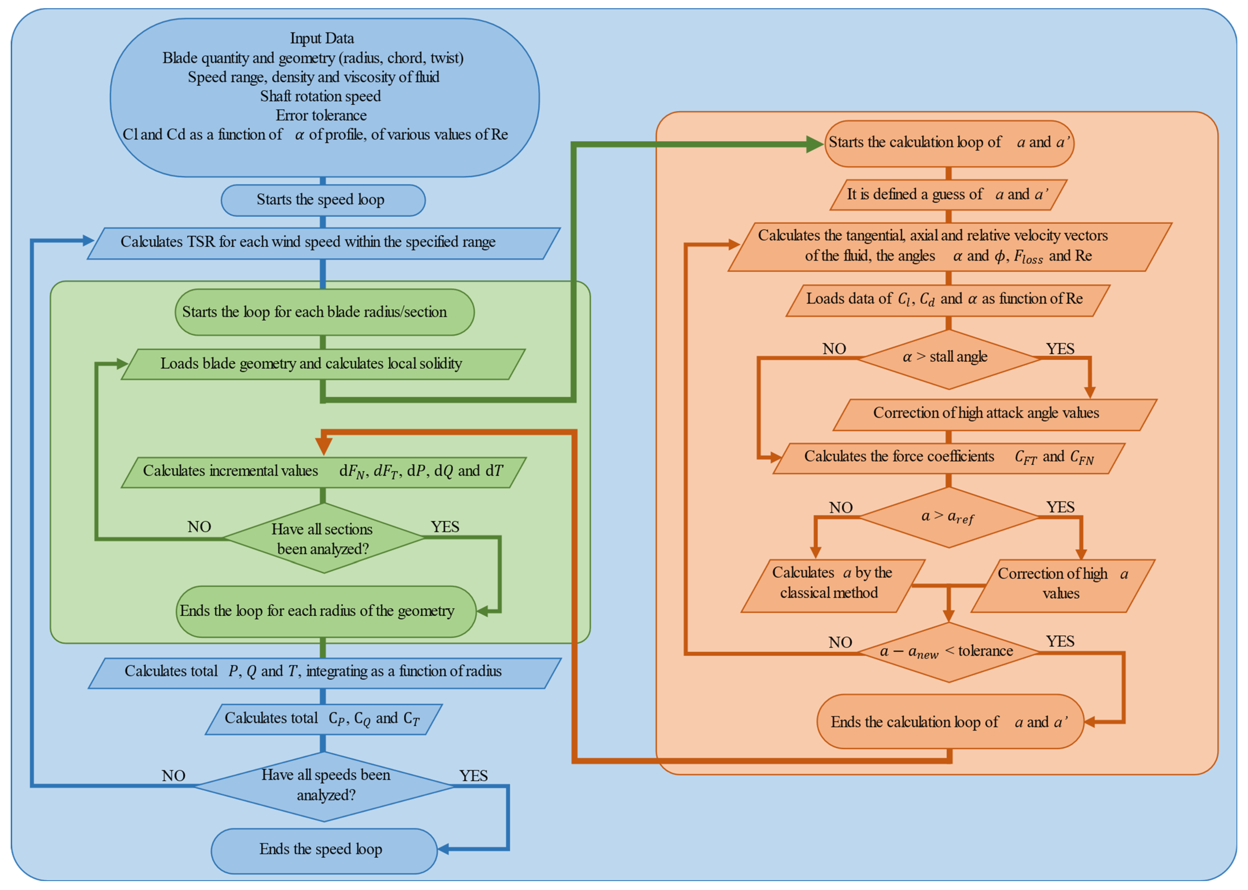
The proposed BEMT algorithm to carry out the simulations of the correction methods is illustrated in the flowchart shown in
Figure 3. Starting from the input data, the algorithm works with three calculation loops: for the fluid velocity (in blue color), for the blade section or element (in green color), and for the axial induction factor (in orange).
The first loop starts by selecting the first fluid velocity value in the desired range to analyze the turbine operation, through which is calculated. The second loop, internal to the first, starts from the first section of the blade. The blade shape is selected as a function of the rotor radius and the local solidity is calculated. The third loop, internal to the second one, is started to iteratively calculate the value of the axial induction factor. Initial guesses are configured for the axial and rotational induction factors in this loop. Based on these initial values, the following variables are calculated: fluid velocity components; angles of , and ; and ; corrections of tip and root losses; corrections of the high values of the angle of attack and and again; force coefficients, and ; correction of high values of the axial and rotational induction factors. Only when the calculation of the axial induction factor reaches the number of allowed iterations or when the error is less than the tolerance does the third loop end and the second loop runs again.
Once the third loop finishes, the increment rates of lift, drag, normal, and tangential forces at the rotor are obtained. Then, the incremental torque, thrust, and power values are calculated. Only when these forces and incremental values are calculated for all blade sections does the second loop end and the first one runs again.
Once the second loop is completed, the integrals of torque, thrust, and power are calculated for the whole blade length, as well as their respective coefficients. The first loop finishes when these integral calculations are made for the whole fluid velocity range.
The main expressions for thrust, torque, power, and power coefficient calculations are those presented in Equations (3)–(6). The thrust coefficient (
) and torque coefficient (
) are calculated by Equations (60) and (61), respectively.
The proposal of this work is based on a methodology whose intention is to combine several correction methods, which are strategically inserted in the Classical BEMT and compiled in the proposed algorithm. The objective is to extract the best results from the possible permutations between methods. From the results obtained, which are discussed in the following sections, it is possible to define and validate a unified model compiled in the algorithm capable of representing horizontal-axis turbines. From now on, this compilation is called the proposed approach, which integrates the following correction: (i) the tip loss correction, proposed by Prandtl; (ii) the induction factor correction, proposed by Shen; and (iii) the angle of attack correction in the post-stall region, proposed by Viterna with Corrigan.
The complementary correction methods are simulated using the algorithm mentioned in the previous subsection. Therefore, it is possible to carry out comparative analyses between them and to define a single structure for the BEMT method (now no longer called classical) that correctly represents the performance of wind turbines in general, regardless of the rated power range.
The small-sized turbine used for the simulations and validation is available in [
20], where further details of design, construction, operation, and performance can also be found. The medium and large-sized turbines used are available in technical reports by NASA, which are Turbine MOD-0 with 100 kW, Turbine MOD-2 with 2.5 MW, and Turbine MOD-5A with 7.3 MW. Design, construction, operation, and performance details can be found in [
21,
22,
23,
24,
25,
26,
27,
28,
29]. It is important to highlight that the methods must represent well the turbine performances, mainly in the region below rated power since the power converters operate at their power limit from that point on. Therefore, the turbine may operate with mechanical torque reduction from that point if the wind speed is available.
3. Results and Discussion
The correction methods are analyzed in separate groups, shown in the following subsections: for the tip loss, for the axial induction factor, and for the angle of attack. First, the results are discussed based on the power curves to evaluate whether the methods correctly represent the performance curve of the turbines. In this way, it is possible to identify the most accurate methods. Additionally, the methods are discussed in terms of power coefficient curves because the errors related to the real data are easier to observe.
3.1. Comparative Analysis of Tip Loss Corrections
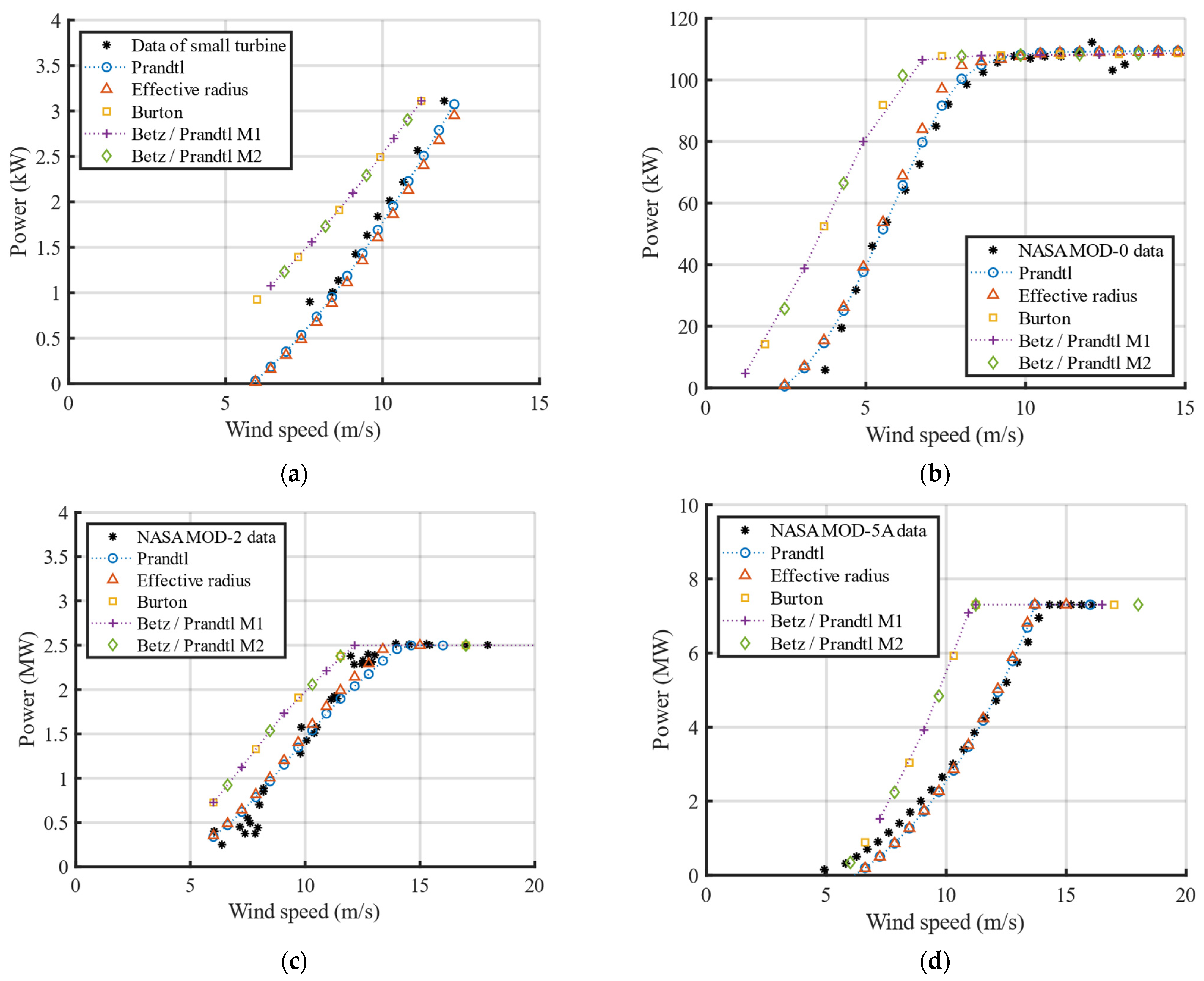
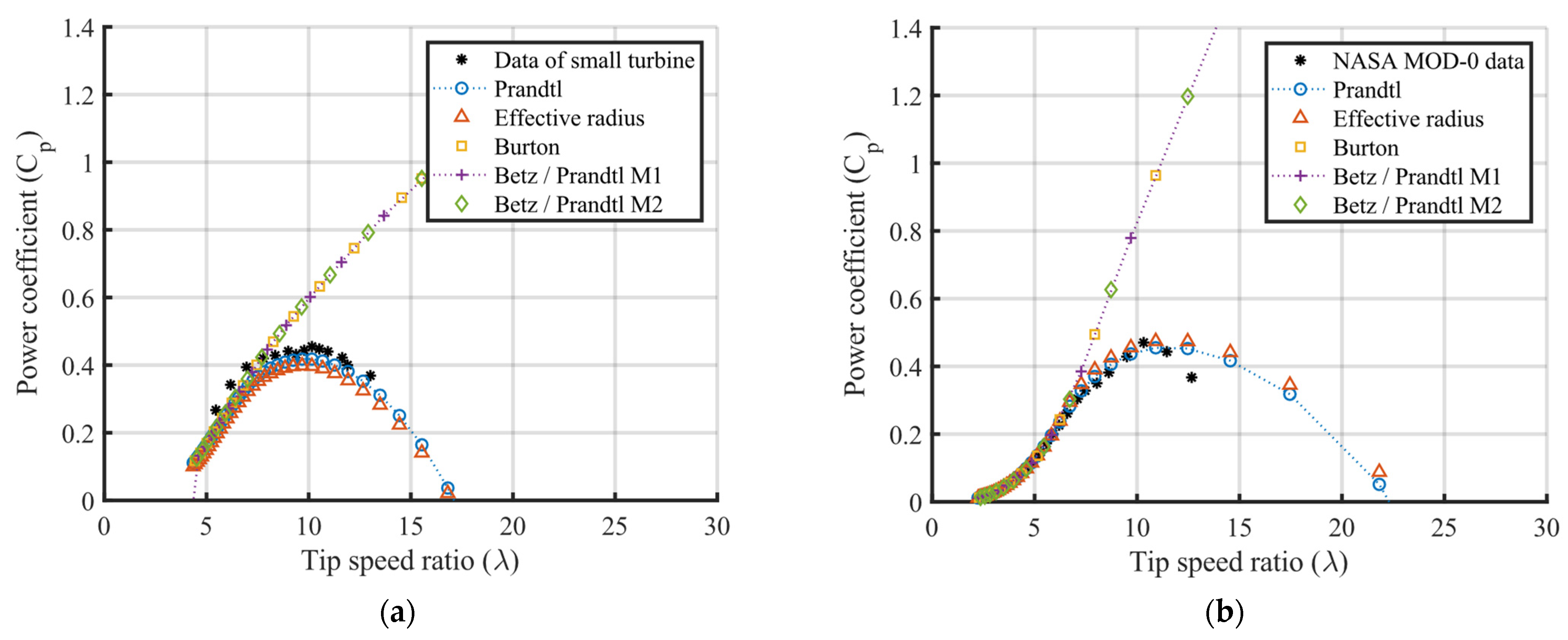
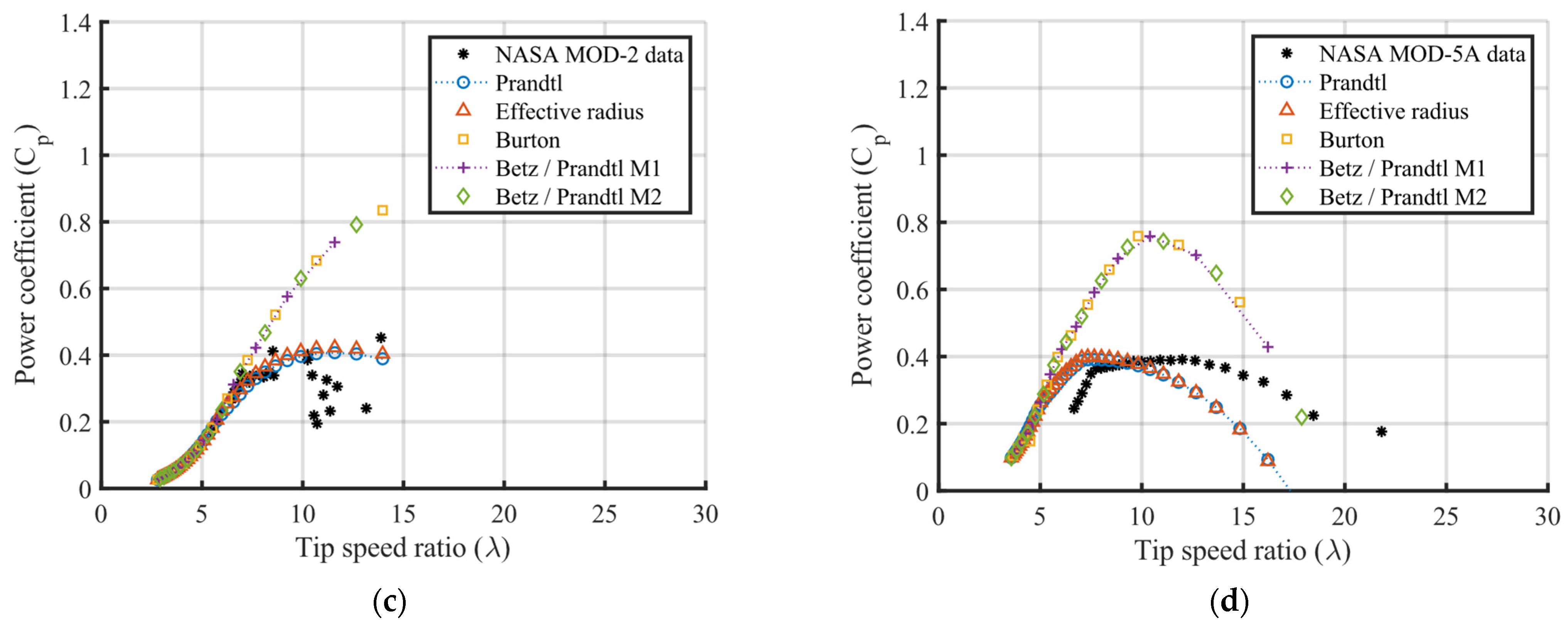
Figure 4 shows that the modeling described by Burton and those by Betz with Prandtl (defined as Prandtl M1 and Prandtl M2), under the same condition, do not correctly represent the power data curve for the four simulated turbines. The results of these methods are similar due to the similarity between the mathematical models used. On the other hand, the other two methods analyzed present results close to the turbine data, and the method described by Prandtl is the closest one. This can be seen more easily in
Figure 4a,b. These results are also observed in
Figure 5, now from the curve of power coefficients, where Burton, Prandtl M1, and Prandtl M2 exceed the Betz limit, being physically inconsistent. In
Figure 5 it is evident that the method described by Prandtl is more assertive than the Effective Radius in relation to turbine data, being more evident for
in
Figure 5a. The modeling described by Prandtl is assumed to be the best for correcting tip loss.
Table 2 shows a summary of the correction methods.
3.2. Comparative Analysis of Induction Factor Corrections
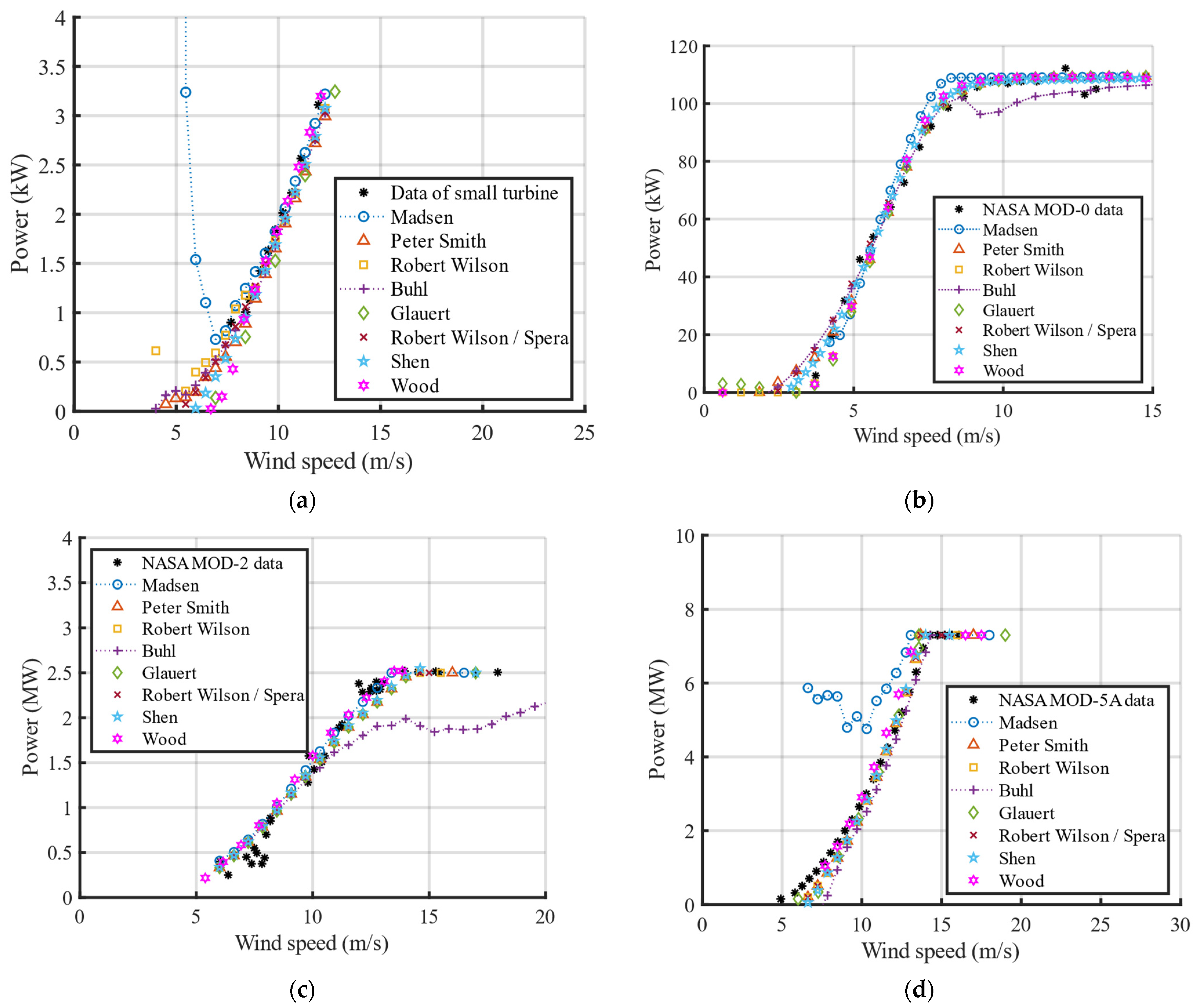
The results presented in
Figure 6 show that the modeling described by Madsen presents significant numerical instabilities for the small turbine in the low wind range (
), as well as big numerical instabilities for the large turbine (MOD-5A) across the entire wind speed range, see
Figure 6d for
. The modeling described by Buhl presents significant errors for the MOD-0 and MOD-2 turbines, specifically for high wind speeds, approximately
. Furthermore, Buhl’s method is the one that presents the biggest error for the MOD-5A turbine data when considering the wind speed range between 5 and 10 m/s.
Considering the results in
Figure 6, the methods described by Peter Smith, Robert Wilson, Glauert, Robert Wilson with Spera, Shen, and Wood present the best results compared to the experimental data.
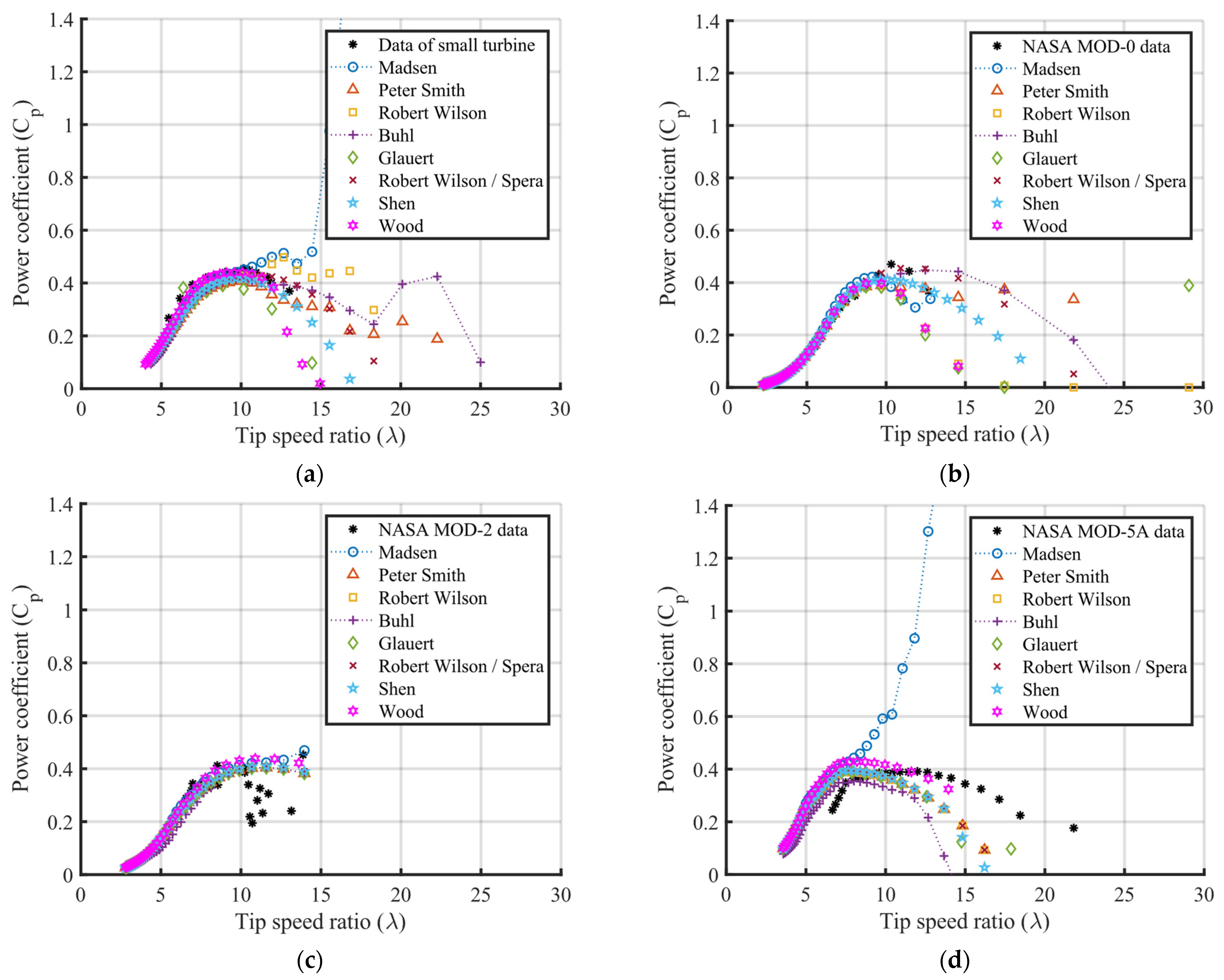
For the small turbine and MOD-0 in
Figure 7b, the methods described by Peter Smith and Glauert show inconsistent results for approximately
, in which
continues to increase after the maximum point of the curve. However, in this region, the
should continuously decrease when λ increases due to, usually, stall conditions on the blades, which leads to a low value of torque and, consequently, a low rotational speed on the turbine axis.
Robert Wilson’s method presents results that oscillate in the range of
for the small turbine shown in
Figure 7a. This highlights the problem of correctly representing the low torque region for high
.
Finally, the models proposed by Robert Wilson with Spera, Shen, and Wood present good
curves. However, the results using Shen’s method are more proximate to the real data from the simulated turbines (see
Figure 7a,b for
). In
Figure 7a,b, for
, the results of Robert Wilson with Spera tend to be somewhat greater than the turbine data. On the other hand, the results of Wood tend to be somewhat lower than the turbine data for
, but all of them, in general, are in good agreement with the experiments.
Based on the simulations performed, it is noticed that the most assertive correction methods for the behavior of the turbines, considering the comparative analysis of induction factor correction, are those in which specific calculations for the induction factor in the low torque region are implemented. The results from the curve confirm this statement.
The method proposed by Wood is based on improving the accuracy of the tip loss calculation in the region of low tip speed ratio below unity. Furthermore, the method calculates the induction factor for the entire length of the blade rather than calculating an average value for the streamtube. This approach is good for any size of turbine, mainly for those where the flow around the rotor has restriction (diffuser-augmented turbines), where the induction axial velocity component is different to the circumferential one. Due to this, the accuracy of this method is good, as it considers the influence of vortices along the blade in a more general form than that using Prandtl. Therefore, taking all this into account, the methods described by Shen and Wood are considered the best ones for correcting the induction factor.
Table 3 shows a summary of the methods.
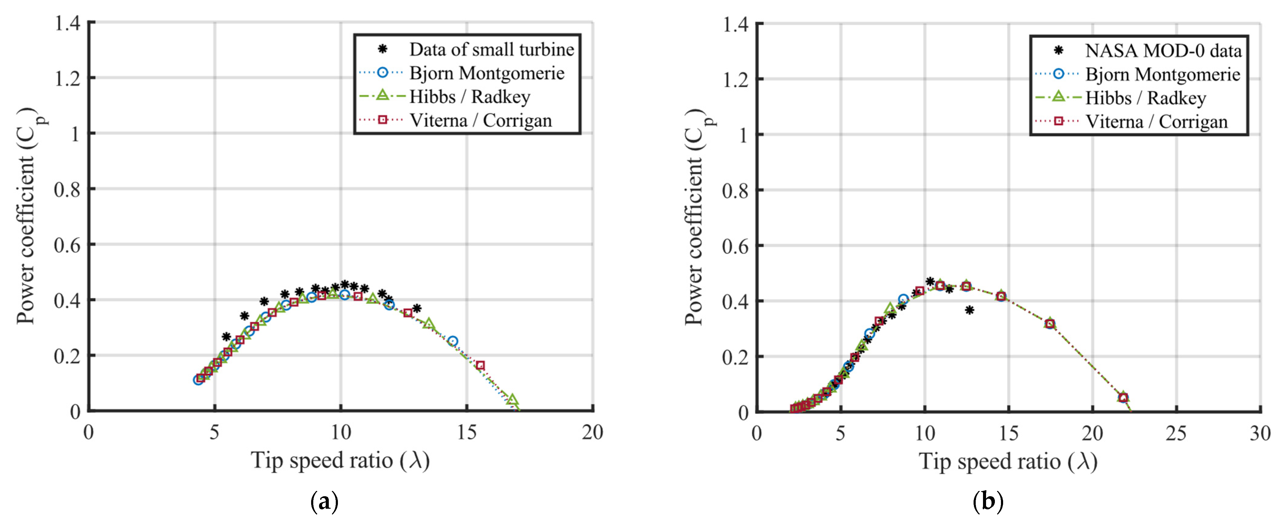
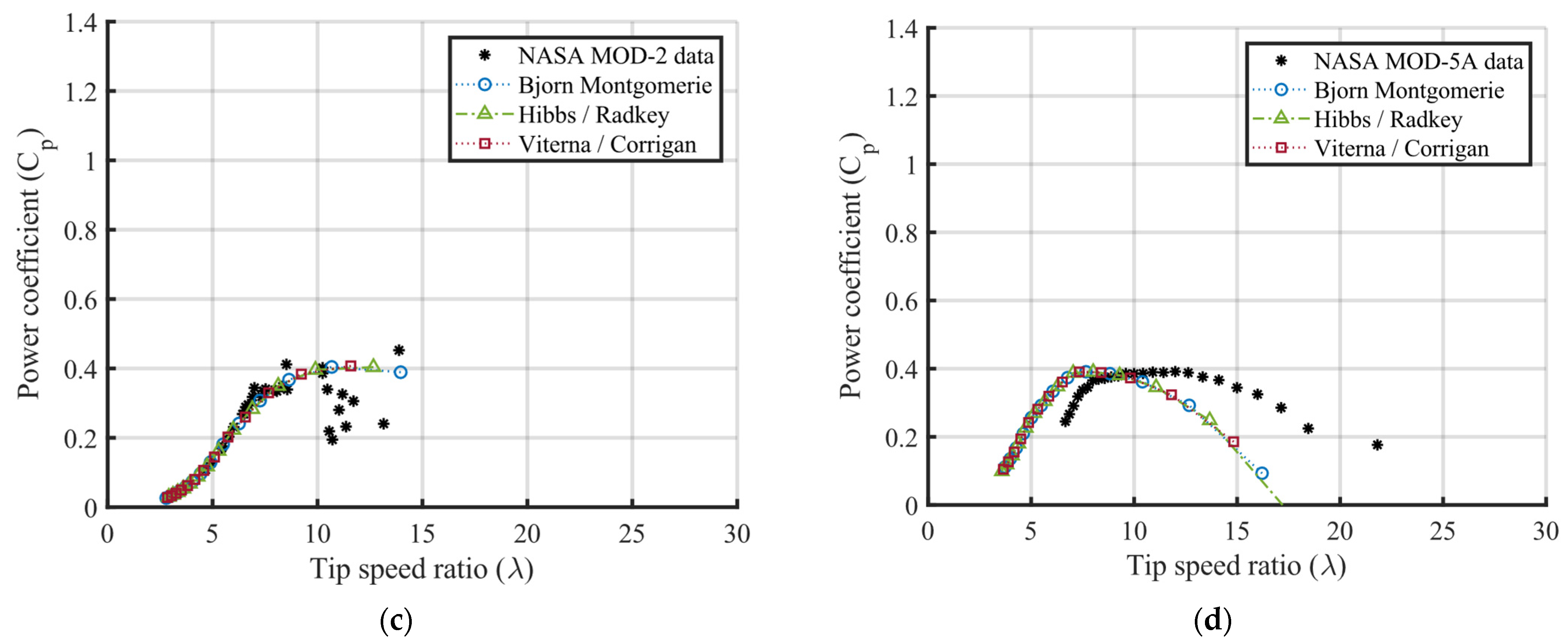
3.3. Comparative Analysis of Angle of Attack Corrections
Among the types of corrections to the classical BEMT, the angle of attack correction is the one that has fewer models. Among those, the mathematical expressions are very similar because all these corrections are based on the post-stall model developed by Viterna and Corrigan.
Montgomerie and Radkey proposed the correction only for the
variable, which considers the drag of the nacelle and the blade. Due to the mathematical similarity between the methods, the results obtained for all simulated turbines are almost the same for the entire wind speed range, as shown in the power coefficient curves of
Figure 8. Furthermore, all the results obtained are close to the data from the simulated turbines. Therefore, any of these three modeling techniques could be used to correct the angle of attack in the post-stall region since the drag effect does not differ a lot between these modeling.
Therefore, the modeling described by Viterna and Corrigan is considered in this article the best modeling for correcting the high values of
. Comparable to the power coefficient curves, the results of those three modeling techniques are almost the same. Thus, it is assumed that the curves of the power coefficients are not needed.
Table 4 shows a summary of the methods.
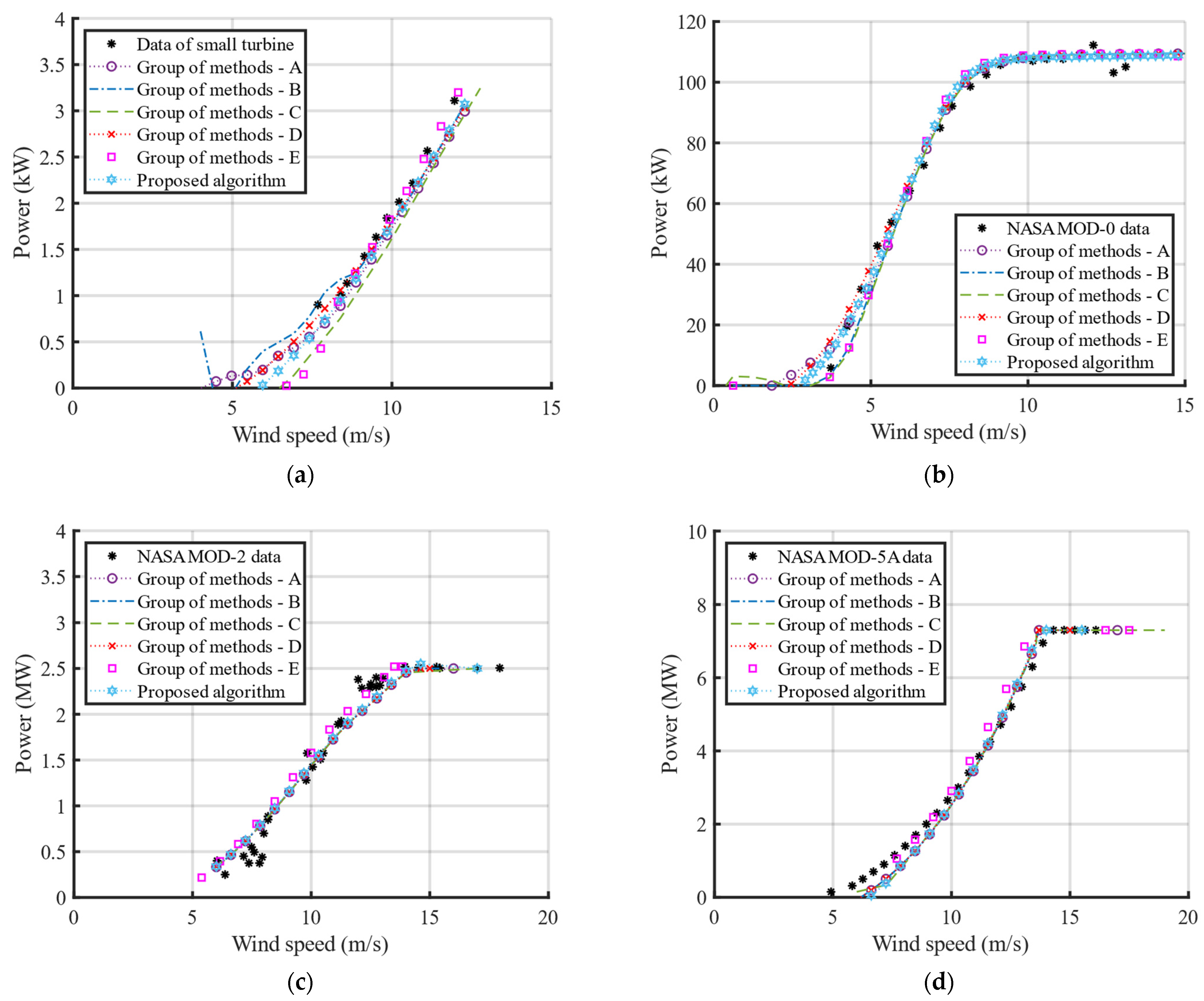
3.4. Comparative Analysis of the Proposed Algorithm
In this subsection, a comparative analysis is performed in terms of numerical instability, in which the correction methods available are submitted to the same operating condition, considering small, medium, and large rotors. Thus, the approach with better numerical stability will be called here the “proposed algorithm”, only for convenience, which is composed of the corrections of Viterna and Corrigan for high angle of attack, the correction developed by Shen for high values of the axial induction factor, which brings very good numerical stability, and that by Prandtl for tip and root losses, due to its easy implementation. All groups shown in the figures are composed of the method Viterna and Corrigan. The groups are A—Peter Smith, B—Robert Wilson, C—Glauert, D—Robert Wilson with Spera, and E—Wood.
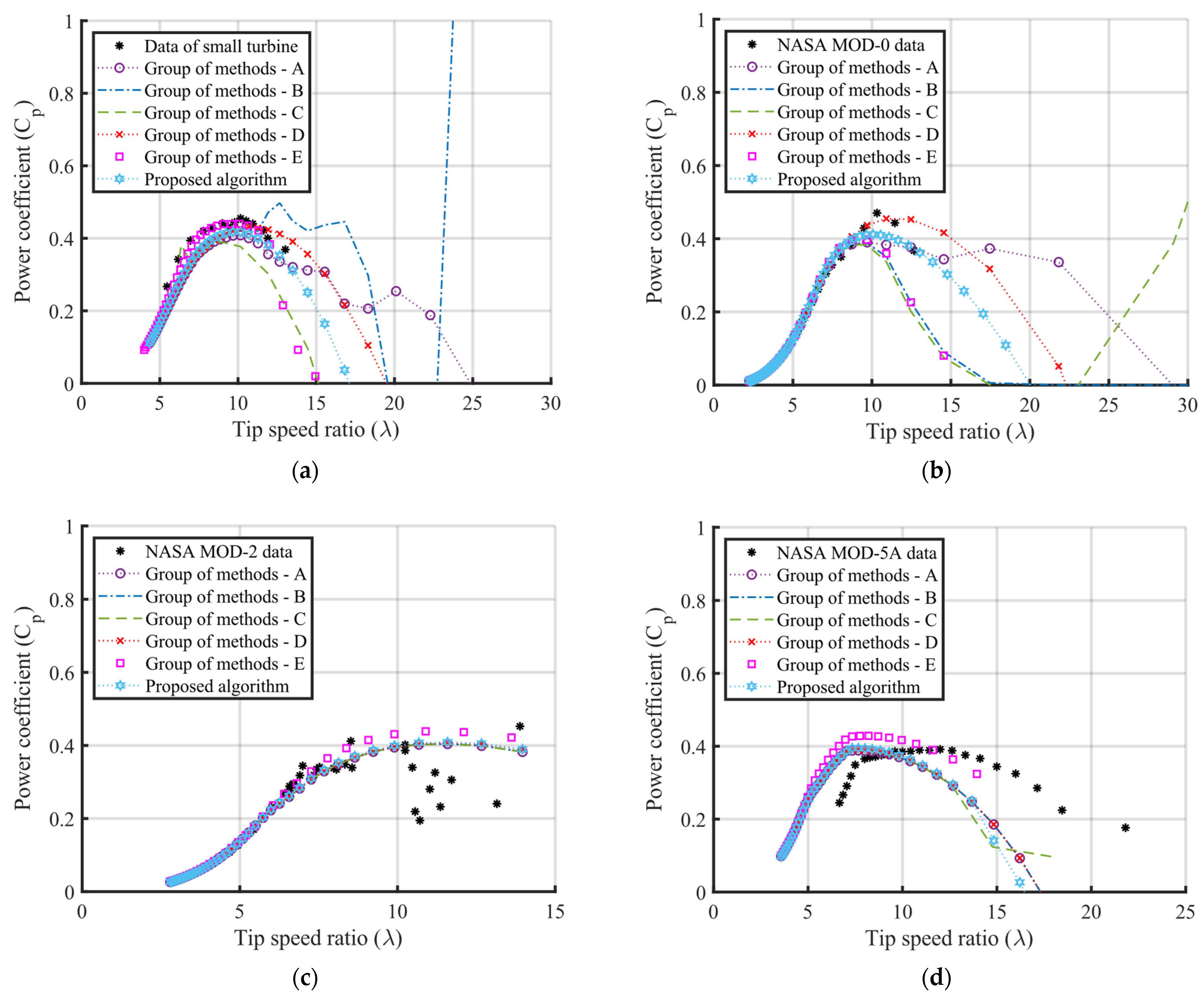
Figure 9a shows that group B presents significant numerical instability at the low-speed region for the small-size turbine. The rest of the groups present good agreement with the experiment, showing similar results between them.
Figure 10a,b clearly show this instability on power coefficient curves for
, where the results of groups are different from each other. The method described by Peter Smith has higher numerical instability for approximately
to small and medium turbines, where
continues to increase after the maximum point of the curve.
Figure 10a,b show that the “proposed algorithm” follows the trend of the turbine data and presents results closer to the real curve than group D.
Therefore, it is correct to say that the results obtained with the “proposed algorithm” correctly represent the real data of the four turbines for the entire wind speed range. This occurs because the model described by Shen et al. [
58] uses two intermediate functions, which are given in Equations (46) and (47), respectively. This condition is used to precisely calculate the induction factors as a function of the radial position at the turbine rotor, taking into account the vortices along the blade. This better predicts the aerodynamic forces in the vicinity of the blade tip, resulting in more accurate power curves.
These intermediate functions combined with the corrections of Viterna and Corrigan for high angle of attack, and that by Prandtl for tip and root losses proved to be, numerically, very stable for predicting the power performance of small, medium, and large turbines than the others presented here.
Table 5 shows a summary of the methods.
Moreover, the alternative method proposed by Wood et al. [
18], using helical vortex theory is very stable. Even though it is more complex to implement, it considers the nonlinear terms in equations of the streamtube for angular and axial momentum, leading to precise results. This method is an accurate way of including these in BEMT calculations [
53], which can be extended for turbines with a diffuser, as it considers a distinguishing between axial and circumferential induction velocities.
The algorithm proposed in this work is efficient and can be used in a generic way to represent the performance of horizontal-axis turbines, from small to large. The main differences between small, medium, and large wind turbines are in rotor design and manufacture. The performance, in terms of power coefficients, of small, medium, and large turbines is very similar, as shown in
Figure 7.
The main challenges for small ones are low operational Reynolds number, as small rotors usually operate at low wind speed; and the structural requirements of more rapidly rotating turbines. Moreover, most small turbines use “free yaw” whereby a tail fin, rather than an automatized yaw drive as on larger rotors, is used to align the turbine with the wind direction. Additionally, usually, small wind turbines do not have pitch adjustment of the blades, making the aerodynamic torque indeed relevant at very low rotational speeds. All these concerns can be implemented using the “proposed algorithm”.
The time of simulation is infinitely lower when compared to the time of simulation of programs that use finite volume analysis such as CFD, so the cost of computational burden is low and consequently requires cheaper computers. The pre-processing of the proposed algorithm is simple because it is based fundamentally on the information of the blade shape (radius, chord, and angle of pitch) and the polar data of the airfoil. In CFD simulation, the pre-processing is complex and involves the three-dimensional design of the blades and nacelle, besides the generation of the mesh to the processing of the calculations based on finite volume analysis. However, it is important to highlight that CFD methods are indeed more robust than those based on BEMT.
4. Conclusions
A simple and fast-processing algorithm capable of estimating the power performance curve for any turbine size is presented. The algorithm is a quick alternative to be applied for predictive studies, ensuring the following aspects: (i) it guarantees widespread application for small, medium, and large-sized wind turbines since the BEMT approaches found in the literature are implemented and adjusted for a specific power range turbine, and cannot be used generically; (ii) fast-processing for performance analysis; (iii) simple implementation when compared to those with CFD modeling, which demand more computational burden and is more complex to simulate; and (iv) it avoids the need for high-performance computers, which are expensive.
In a general context, a summary of the application of existing methods is presented as follows: (i) the correction methods of tip losses proposed by Prandtl and the one of Effective Radius can be applied to any turbine size since the results approximately represent the power curve data; (ii) the correction methods of induction factor proposed by Shen, Wood, and Robert Wilson with Spera can be applied to any turbine size. The methods proposed by Peter Smith and Robert Wilson can be applied to medium and large turbines; (iii) the correction methods of the angle of attack proposed by Bjorn Montgomerie, Hibbs with Radkey, and Viterna with Corrigan can be applied to any turbine.
However, the proposed algorithm presented and discussed in the flowchart shown in
Figure 3 is composed of the corrections of Viterna and Corrigan for high angle of attack, by Shen for high values of the axial induction factor, and by Prandtl for tip and root losses. It is essential to highlight that the method proposed by Wood is more accurate for low tip speed ratio, mainly for small turbines, as shown in
Figure 7a for
. Moreover, it can be extended to turbines with a diffuser. Therefore, it can perfectly replace Shen’s intermediate functions in the proposed algorithm.
From the results obtained, mainly in the power curves, it is observed that the proposed algorithm performs better in any operating conditions. The algorithm obtained the best approximations for the power curves against the measured values of all turbines, ensuring a wide application. As the simulation takes a few seconds, it proved to be effective and quick for turbine analysis. In addition to having less complexity, it can be very well applied generically for predictive studies without needing additional adjustments or corrections. Furthermore, the prior need for high-performance computers to analyze turbine power coefficient is avoided.
For future work, it is important to extend the studies to assess the effect of the turbine powertrain, in order to evaluate the influence of the electrical generator on the rotor behavior in terms of time constant. Controllers implemented in power converters for wind turbines depend on this time constant to improve the dynamic response of the system.

 ,
, 


