Research on the Sustainable Development Path of Regional Economy Based on CO₂ Reduction Policy

Abstract

With the rapid growth of China’s economic growth, a large number of greenhouse gas emissions have led to a significant increase in environmental pressure. Currently, China has not yet achieved a good balance between greenhouse gas emissions and economic growth. To improve the sustainable development of China’s regional economy and effectively control domestic CO₂ emissions, research is conducted to analyze the trend of regional economic change based on carbon emission policies. This study looks for suitable paths to achieve sustainable development of the regional economy. In this study, CO₂ emissions were incorporated into an economic model to calculate the Green Total Factor Productivity (GTFP) efficiency value and its growth rate in each region of China. This was done to examine the productivity of each region in China. and it also aims to discuss the driving factors behind it, so as to give relevant policy suggestions that can help China’s sustainable economic development. The ultimate goal is to achieve sustainable RE development. The method used to measure the GTFP efficiency was the slacks-based measure (SBM) based on the data envelopment analysis (DEA) technique. The regression analysis of the relevant drivers was based on the regression analysis of the panel data model. The research results show that the level of urbanization and industrial structure were the main influencing factors for the increase of CO₂ emissions. Consequently, macro-regulation can appropriately reduce CO₂ emissions. In addition, the implementation of carbon emission reduction policies such as industrial structure optimization, education investment, and market-oriented reform also promote the sustainable development of the regional economy. Therefore, appropriate carbon emission reduction policies can improve the level of sustainable development of the regional economy. It also can ensure the stability of the regional environmental level.

1. Introduction

Under the development strategy of China’s industrial structure, which is dominated by heavy industry, the economic growth rate of China has increased greatly [1,2]. The ensuing environmental pressures pose a huge challenge to the Sustainable Development (SD) of China’s economy [3]. Among them, the growth of carbon emissions and environmental pollution have a great impact on the SD of the economy. Hence, China has formulated a series of emission-reduction policies to control carbon emissions to alleviate the environmental pressure [4,5,6]. Green Total Factor Productivity (GTFP) is a total factor measurement system that removes non-desired outputs and represents the level of SD of regional economies [7,8]. In this context, China’s regional economic level will more or less change with the adjustment of carbon emission reduction policies. Therefore, it is of important practical significance to analyze the internal relationship between carbon emission reduction policies and sustainable development of the regional economy. Currently, many studies have provided many methods to improve the sustainable development of the regional economy. For example, Li et al. proposed a new two-stage stochastic interval parameter fuzzy programming strategy model. This model is based on the water environment system and aims to improve the sustainable development of the regional economy and environment. The model can solve the complexity and uncertainty of water supply systems. The method is applied to planning resource management and developing regional environmental sustainability. The results can not only help decision makers formulate resource-allocation strategies, but also provide insight into the benefits of economic and environmental objectives [9]. In addition, the Smyslova team has established a system based on modern geographic information system technology. This was done to improve the sustainability of socioeconomic development and address the low level of socioeconomic development in the region. The research indicates that using geographic information systems in formulating measures to improve sustainable socioeconomic development of a region can promote the quality of complex system state analysis. This system is not only essential to addressing practical issues in allocating resources or analyzing the effectiveness of resource deployment, it also helps to implement strategic planning principles using digital technology and ensure the timeliness of decisions made in the field of investigation [10]. However, there are few studies that combine sustainable development of a regional economy with carbon-reduction policies. Therefore, this study combines the two to not only fill the gap in this research but also provide practical strategies for achieving sustainable development of a regional economy. With the development of empirical models, research on SBM models and DEA techniques is also increasing. In order to objectively calculate the efficiency of provincial green innovation, Li proposed an SBM model based on DEA technology and fuzzy evaluation and used this model to calculate the green innovation efficiency of 30 provincial industrial enterprises. The results showed that this model improves the accuracy and authenticity of the evaluation of green innovation economic efficiency [11]. In order to better calculate the sustainable development of a regional economy, DEA technology and SBM model have also been applied in the study. This method not only provides a new testing method for the calculation of regional economic sustainable development but also provides new ideas for exploring regional green sustainable development. In addition, the study also expresses the level of sustainable development of a regional economy through green total factor productivity, which not only provides a new indicator for sustainable development of a regional economy but also improves its level of sustainable development by promoting the growth of green total factor productivity, providing new methods for improving the level of sustainable development of a regional economy. Hence, this research analyzes the influencing factors of green total factor productivity and its growth rate through static and dynamic regression model analysis and econometric empirical models. It hopes to provide some appropriate carbon emission reduction policy recommendations through the analysis results, making contributions to the sustainable development of China’s regional economy. Through this study, the following two theoretical gaps with current research are found. The first point is that carbon emission reduction policies and regulations can indeed effectively improve the sustainable development level of regional economies. The second point is that different carbon emission reduction policies and regulations have different effects on the sustainable development of regional economies.

2. Correlation Analysis between Carbon Emission Reduction Policy and SD RE

2.1. Correlation Analysis between GTFP and RE Sustainability

The regional economy is linked to the productivity of the region. The higher the productivity, the better the regional economy. It is usually expressed by total factor productivity [12]. However, green development and SD are gradually emphasized by all sectors of society. Therefore, a GTFP, which includes non-desired outputs such as carbon emissions in the index system, can more objectively describe the regional economy than total factor productivity that only considers desired outputs [6,13,14]. Sustainable RE development refers to the pursuit of not only the quantity of economic development, but also the assurance of quality in its development process. This is to achieve cleaner production and civilized consumption, thereby improving the efficiency of economic activities. Ultimately, it is meant to realize an intensive economic growth mode [15,16]. From the meaning of sustainable development of a regional economy (SD RE) and green total factor generation rate, the latter has a positive promotion effect on the former. This means that a region’s degree of economic SD increases with its GTFP.

2.2. Correlation Analysis of Carbon Reduction Policies and GTFP

Carbon emission reduction policy is formulated by the state to reduce CO₂ and related greenhouse gas emissions. These mainly include policies on adjusting and optimizing industrial structure, increasing investment in technology development, controlling CO₂ increment, innovation models, etc. At present, carbon emission reduction policies include carbon emission tax policy, carbon trading policy, renewable energy policy, and so on. The government macro-regulates energy consumption through CRPs to reduce undesired output [17,18,19]. GTFP is primarily a total factor measuring system. It is used to assess industrial development and economic progress while including resource consumption and environmental pollution as measurement indicators into input components [20,21]. The influencing factors of green total factor productivity include technological innovation, management innovation, and the degree of openness to the outside world. The lower the level of non-desired outputs such as carbon emissions and energy consumption, the higher the GTFP [22]. Therefore, an increase in GTFP indicates a decrease in carbon emissions and energy consumption, so the implementation of carbon emission reduction policies can improve green total factor productivity. That is, the higher the implementation of carbon emission reduction policies in the region, the higher the corresponding increase in green total factor productivity in the region.

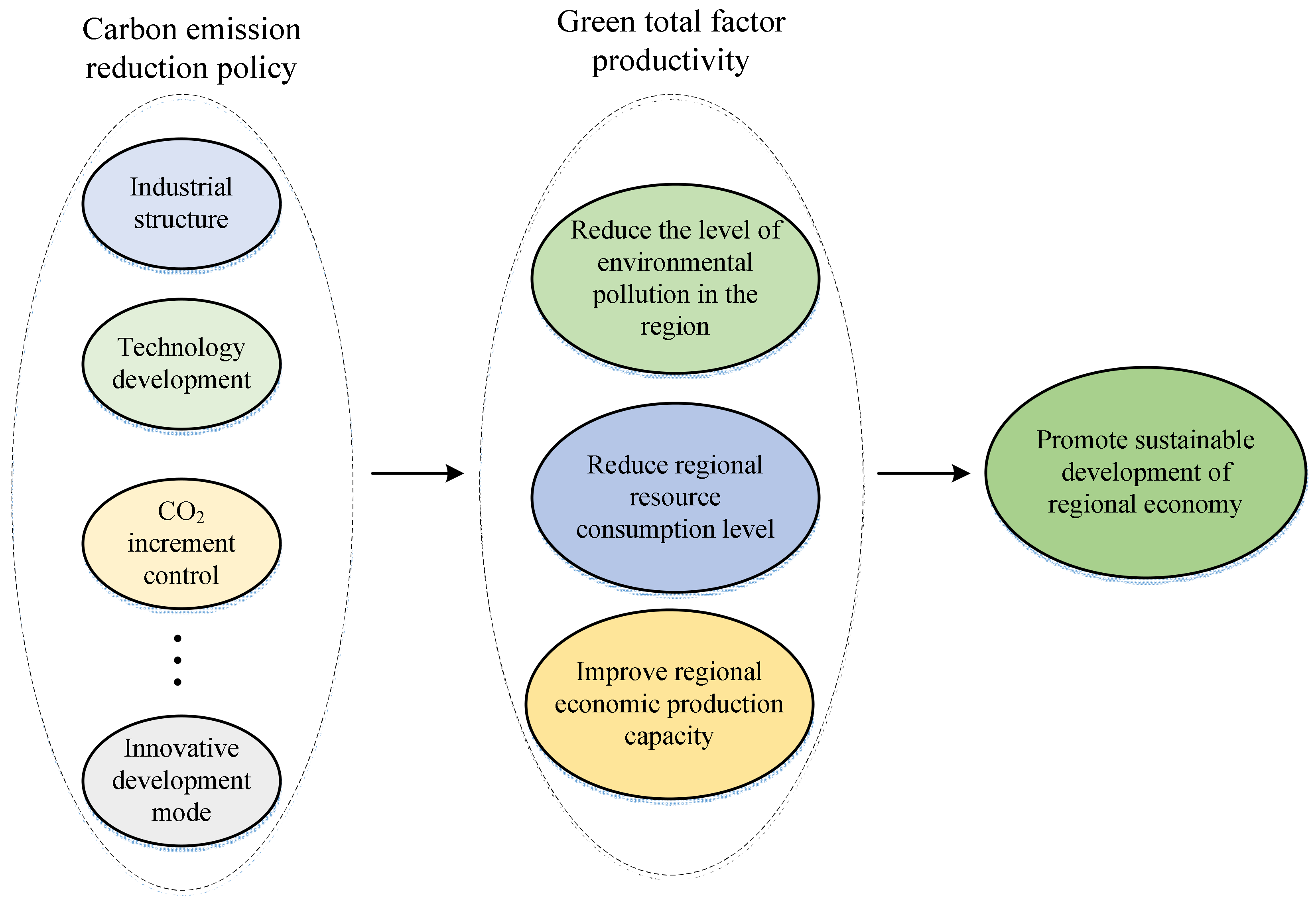
2.3. Analysis of the Impact of CRPs on the SD of a Regional Economy

Through the above analysis of the relationship between GTFP and SD RE, and the relationship between carbon emission reduction policy and GTFP, the analysis of the impact of carbon emission reduction policy on SD RE could be obtained. It is indicated in Figure 1.

As can be seen in Figure 1, various regions implement carbon emission reduction policies in terms of structural adjustment, increasing technological development, and controlling the CO₂ increment. This has achieved the goals of improving regional economic production capacity, reducing energy consumption levels, and reducing environmental pollution levels. Thus, the GTFP of the region will be improved, and the SD of the region’s economy will be promoted. The above analysis leads to the hypothesis that appropriate carbon reduction policies have a positive impact on the SD of a regional economy. This hypothesis was verified by establishing several econometric and regression models for analysis.

3. Empirical Study of CO₂ Emissions in Various Regions

3.1. Emission Measurement Model Construction for Each Region’s CO₂

To measure the GTFP efficiency values and their growth rates in each region better, the study incorporated the CO₂ emissions of each region into the economic model. The data used in the study were panel data from various provinces in China from 2001 to 2020. Among them, the fixed price GDP of each province in 2000 was the output indicator; the number of employees in the whole society of each province was the labor factor input indicator; the total energy consumption of each province was the energy factor input indicator. The above variable data were derived from the “China Energy Statistical Yearbook” and various regional statistical yearbooks over the years. In calculating the CO₂ emissions of each region, the consumption of seven different fossil energy sources and the CO₂ emissions generated by cement production were summed. The expressions are shown in Equation (1) [23].

$$C_{it}={\displaystyle \sum _{l=1}^{l=7}{E}_{itl}\times NC{V}_l}\times CE{F}_l\times CO{F}_l\times (44/12)+Q_{it}\times E{F}_{cement}$$

(1)

In Equation (1), $E$ denotes fossil energy consumption; $NCV$ denotes average low-level heat generation; $CEF$ denotes the carbon emission factor; $COF$ is the carbon oxidation factor; $Q_{it}$ denotes cement production; $E{F}_{cement}$ represents the CO₂ generated per ton of cement produced. Panel data regression models are divided into static and dynamic models. The static panel depicts an economic scenario in which independent variables and dependent variables react instantaneously without time lag. The dynamic panel reflects that, in addition to the explanatory variables having an impact on the explained variables, the previous period base of CO₂ emissions also has an impact on the current period due to the hysteresis of economic variables. Logically speaking, economic development should pay special attention to the continuity of industrial development and the rigid demand for energy [24]. These also determine that China’s CO₂ emissions are unlikely to undergo short-term abrupt changes. Therefore, it is believed that the dynamic panel regression model (incorporating CO₂ emissions from the previous period into the explanatory variable) is more suitable for fitting scenarios in the real economy and has more explanatory power. To better analyze the drivers of carbon emissions in each region, the study used both static and dynamic panel data regression models for regression. The expression of the static model is shown in Equation (2).

$$\ln c{o}_2{}_{{}_{it}}=\alpha +\beta X_{it}+{\eta }_i+{\epsilon }_{it}$$

(2)

In Equation (2), $\alpha$ represents the intercept term; $\beta$ represents the regression coefficient; ${\eta }_i$ represents the individual effect, which represents the difference between different provinces; ${\epsilon }_{it}$ is the disturbance term; $X_{it}$ is the explanatory variable. The expression of the dynamic model is shown in Equation (3).

$$\ln c{o}_2{}_{{}_{it}}=\alpha +\lambda \ln c{o}_{2i(t-1)}+\beta X_{it}+{\eta }_i+{\epsilon }_{it}$$

(3)

The biggest difference is that the static model has no time lag, while the dynamic model has a lag. Hence, the study concludes that the dynamic model is a better fit for the actual carbon emissions in China. To justify this hypothesis, the static model and the dynamic model are regressed for comparative analysis. Both of them use the generalized moment estimation method for estimation. The generalized moments estimation method allows for the elimination of individual effects in the dynamic model. The equation shown in Equation (4) can thus be obtained.

$$\mathsf{\Delta }\ln c{o}_2{}_{{}_{it}}=\lambda \mathsf{\Delta }\ln c{o}_{2i(t-1)}+\mathsf{\Delta }\beta X_{it}+\mathsf{\Delta }{\epsilon }_{it}$$

(4)

At this time, the correlation between $\mathsf{\Delta }{\epsilon }_{it}$ and $\mathsf{\Delta }\ln c{o}_2{}_{{}_{it}}$ remains; $\mathsf{\Delta }\ln c{o}_2{}_{{}_{it}}$ is an endogenous variable. To address this issue, the study selected the second-order differences as the instrumental variable and examined the validity of the instrumental variable by the Sargan test.

3.2. Model Variable Selection

After constructing the regression model, the variables need to be selected, and the study selected several model variables according to the specific situation, as shown in Figure 2. In the study, based on previous research experience and according to the current regional economic development situation, six variables were selected as explanatory variables. They have a significant influence on carbon emissions [25].

In Figure 2, the study selected CO₂ emissions as explanatory variables, in addition to variables such as per capita income, urbanization level, and industrial structure. The per capita income variable was introduced into its cubic model, and the cubic, quadratic, and primary terms of the logarithm of per capita income were used as explanatory variables, respectively, to better explain the model. Light and heavy industries, represented by manufacturing, will consume more energy and have a greater impact on the environment than agriculture and services. The ratio of GDP of the secondary industry was used here. Urbanization is the biggest era background in recent China. The advancement of urbanization has brought about a huge demand for energy and building materials; the demand for energy and industrial products by urban residents is far greater than that of rural areas. Logically, it will lead to an increase in CO₂ emissions, but it is also a huge driving force for China’s economic growth. Therefore, urbanization is included in the explanatory variable and expressed as the proportion of urban residents to the total population. Energy intensity is the energy consumption required per unit of GDP output, reflecting the level of science and technology and the efficiency of energy utilization. It is an indicator of comprehensive factors. This indicator logically connects economic development and energy consumption and is the focus of energy conservation and emission reduction. The explanatory variable of foreign investment is to explain the transfer of polluting industries to China by foreign investors. Finally, the explanatory variable of time trend is an explanation of the progress of science and technology.

3.3. Econometric Model Results and Regression Analysis

The total CO₂ emissions and CO₂ emission intensity of each province and city during 2001–2020 were obtained by the econometric model, as shown in

Table 1. Total CO₂ emissions and CO₂ emission intensity in each region from 2001 to 2020.

Region	Province	Total Carbon Emissions	Carbon Emission Intensity
		Average Value/10,000 t	Average/(t·1000 USD−1)
Central region	Henan	50,215.08	0.38
	Shanxi	70,213.21	1.05
	Anhui	29,366.27	0.85
	Hubei	31,187.19	0.88
	Jiangxi	17,356.38	1.49
	Hunan	26,032.23	0.58
Western Region	Shanxi	30,957.62	0.89
	Sichuan	27,513.62	0.60
	Yunnan	19,585.07	0.28
	Guizhou	21,978.53	1.11
	Guangxi	16,935.68	0.64
	Gansu	17,215.43	0.40
	Qinghai	3796.38	0.35
	Ningxia	13,816.08	2.18
	Xinjiang	28,958.31	0.69
	Inner Mongolia	54,529.76	1.51
	Chongqing	11,127.35	0.52
	Liaoning	60,348.19	0.45
	Heilongjiang	31,219.56	0.82
	Jilin	23,065.46	2.16
	Hainan	3708.56	0.94
	Guangdong	50,489.46	0.83
Eastern Region	Hebei	69,518.35	3.76
	Beijing	13,158.49	0.75
	Tianjin	16,236.35	0.99
	Shandong	93,527.15	0.49
	Jiangsu	59,872.59	1.37
	Shanghai	24,926.73	0.67
	Zhejiang	37,654.28	0.42
	Fujian	20,368.18	0.95

.

In Table 1, Shanxi, Henan, Anhui, Hubei, Jiangxi, and Hunan belong to the central region of China; Shaanxi, Sichuan, Yunnan, Guizhou, Guangxi, Gansu, Qinghai, Ningxia, Xinjiang, Inner Mongolia, Chongqing, and Tibet belong to the western region of China; Hebei, Beijing, Tianjin, Shandong, Jiangsu, Shanghai, Zhejiang, Fujian, Guangdong, Hainan, Jilin, Heilongjiang, and Liaoning belong to the eastern region of China. According to Table 1, the top three provinces in terms of total carbon emissions were Shandong, Shanxi, and Hebei, with 935.2715 million tons, 702.1321 million tons, and 695.1835 million tons, respectively. In addition, it can be seen that the top three provinces in terms of carbon emission intensity were Hebei, Ningxia, and Jilin, with 3.76 t·1000 USD⁻¹, 2.18 t·1000 USD⁻¹, and 2.16 t·1000 USD⁻¹, respectively. From Table 1 and the above results, it can be seen that there were significant differences in carbon emissions and intensity among the regions in China. The regions with higher carbon emission intensity were mostly located in the central and western regions of China. The western region especially had the most provinces with higher carbon emission intensity. Most regions with lower carbon emissions were located in the eastern region of China. After getting the carbon emissions of each region, regression was carried out by using the static model and the dynamic model to get the results. It is indicated in

Table 2. Regression results of the two models.

Explanatory Variable	Static Model	Dynamic Model
CO2 emissions in the previous period	/	0.46 *** (0.06)
Per capita income logarithm	12.28 *** (0.08)	10.19(0.07)
Quadratic power of logarithm of per capita income	1.19 ** (0.68)	1.08 (1.12)
Cubic power of logarithm of per capita income	−0.091 ** (0.48)	−0.61 ** (0.75)
Industrial structure	0.32 ** (0.17)	0.09 ** (0.18)
Energy intensity	−0.14 ** (0.04)	−0.41 ** (0.24)
Foreign investment	0.12 * (0.13)	0.37 * (1.18)
Urbanization level	1.61 * (0.49)	1.99 ** (0.24)
Time	−0.06 ** (0.02)	−0.06 ** (0.02)
Square of time	0.11 ** (0)	0.10 ** (0)
Constant term	−0.21	0.04 ** (0.25)
Estimation method	Generalized least squares	Generalized moment estimation
Arellano	/	−3.38 *
Sargan test	/	57.46
Adjusted R2	0.78	0.93
AIC	−3.58	−4.03
BIC	−3.49	−4.47

Note: The superscripts *, **, *** indicate significance at 10%, 5%, and 1% confidence levels, and standard errors are in parentheses.

.

Table 2 illustrates that the overall fit of the dynamic model was better than that of the static model, which verifies the previous hypothesis. The level of urbanization and industrial structure were found to be the main paths of CO₂ emissions in the dynamic model. These two are mainly regulated through national policies. Energy intensity is the variable that had a suppressive effect, and carbon emissions could be reduced by improving the input on energy intensity. The regression coefficients of industrial structure variables revealed that the industrial structure is unreasonable and needs to be adjusted urgently. In addition, the foreign investment variable indicated that the government should not blindly attract investment for the sake of economic growth.

4. Measurement and Analysis of GTFP Efficiency Values

4.1. Selection of Efficiency Measurement Model

To measure the efficiency of GTFP, the slacks-based measure (SBM) model based on data envelopment analysis (DEA) technique was chosen. The DEA technique is widely used in energy and environmental efficiency measurements because it can deal with the efficiency measurement of multiple inputs and outputs [26,27]. However, traditional DEA models cannot distinguish between desired and undesired outputs, which makes the measurement of production efficiency inaccurate [28,29]. The SBM model, on the other hand, can directly put the slack variables into the objective function. It solves the problem of DEA techniques ignoring slackness. The specific expression of the SBM model based on the DEA technique is shown in Equation (5).

$$\{\begin{array}{c}\min p_0=\frac{1-\frac{1}{N}{\displaystyle {\sum }_{n=1}^N{S}_n^{-}/x_{n0}}}{1+\frac{1}{M+J}({\displaystyle {\sum }_{m=1}^M{S}_m^{+}/y_{m0}}+{\displaystyle {\sum }_{j=1}^J{S}_j^{-}/u_{j0}})}\\ s.t.{\displaystyle \sum _{k=1}^K{z}_k{x}_{nk}}+S_n^{-}=x_{n0},n=1,2,\cdots N\\ {\displaystyle \sum _{k=1}^K{z}_k{y}_{mk}-S_m^{+}=y_{m0},m=1,2,\cdots M}\\ {\displaystyle \sum _{k=1}^J{z}_k{x}_{jk}+S_j^{+}=x_{j0},j=1,2,\cdots N}\\ z_k\ge 0,S_n^{-}\ge 0,S_m^{+}\ge 0,S_j^{-}\ge 0,k=1,2,\cdots K\end{array}$$

(5)

In Equation (5), $p_0$ denotes the SBM efficiency value; $x$ and $y$ denote the input vector; $K$ denotes the decision unit; $S_n^{-}$ and $S_m^{+}$ are slack variables; $u$ denotes the undesired output vector; $S_j^{+}$ denotes the undesired output residual. The model also enables the calculation of optimal solutions for factor inputs and expected generation. Therefore, the model to account for GTFP efficiency values and the obtained efficiency values are analyzed empirically to identify the drivers.

4.2. Measurement of the GTFP Efficiency Value

Since the focus is on measuring the GTFP of each region from 2001 to 2020, the main expected and undesired outputs were the real GDP and CO₂ emissions of each region, respectively. Capital, labor, and energy consumption factors were the input factors. The data of labor indicators were obtained from the employees. The data of energy consumption indicators were obtained from the total energy consumption of each region. The emission indicators were obtained from the CO₂ emissions of each region. Using Equation (5) to process the accessed data accordingly, the GTFP could be obtained for the corresponding year. Figure 3 shows the GTFP efficiency values in the eastern and western regions during the period 2000–2020.

Figure 3 showcases that the overall level of GTFP in the eastern regions of China was higher than that in the central and western regions. It shows that the better the economic situation, the higher the GTFP. In addition, the overall GTFP of all regions was on an upward trend with the growth of years. The GTFP of all regions was higher than 90% by the end of 2020. This result indicates that under the guidance of China’s low carbon policy and public opinion, the GTFP of China has improved significantly.

4.3. Analysis of the Drivers of GTFP Efficiency Values

After obtaining the GTFP, to analyze the factors that influence the GTFP in the country, the study used an econometric model to analyze it by regression. GTFP consists of two components: resource reallocation efficiency and micro-production efficiency. The efficiency of resource redistribution is mainly determined by industrial restructuring and the marketization process. Micro-generation efficiency is mainly determined by new technologies and management practices [30,31,32]. Therefore, the study selected marketization variables, research and development investment, the logarithmic value of imported foreign expenditure, foreign investment, and years of education per capita as explanatory variables to construct the model. Marketization variables comprehensively reflect the regulatory role of the market on the economy and the allocation of factors. They are also the main direction of market-oriented reform led by the government in China and have a relatively obvious incentive effect. Therefore, they are considered as typical institutional variables. Research and development investment is used to examine the impact of China’s independent research and development investment on green total factor productivity. More investment in research and development of new technologies will logically lead to production technologies that are more conducive to improving production efficiency. Therefore, there is reason to believe that R&D investment will affect actual production efficiency, so it is included in the explanatory variable. The natural logarithm of expenditure on introducing foreign funds is the expenditure variable for purchasing foreign technology. In fact, in addition to independently developing new production technologies, it is easier to achieve the effect of improving production by directly purchasing production technologies that are conducive to improving production efficiency from abroad. Therefore, there is reason to believe that the cost of foreign technology purchases will affect China’s green total factor productivity. Therefore, this indicator was selected as an explanatory variable. FDI refers to the degree of foreign trade. When foreign investors invest in establishing factories in China, they inevitably communicate and exchange information with the location of the factory. This will promote the improvement of the production efficiency of domestic enterprises within the investment location. In addition, foreign investment has attracted a large number of local unemployed residents to obtain employment and provided them with higher wages. To some extent, it has also provided them with more efficient production technology and higher production efficiency. Therefore, it is necessary to include foreign investment in the explanatory variables. Edu is the number of years of education per capita, used to examine the impact of human capital on green total factor productivity. The length of education actually determines the level of education received. Although not everyone will become skilled after education, in fact, the level of public education will affect the probability of the emergence of top talent and the overall productivity of the entire society. The constructed econometric model is shown in Equation (6).

$$TF{P}_{it}={\beta }_0+{\beta }_i+{\beta }_j{X}_{jt}+{\epsilon }_{it}$$

(6)

In Equation (6), $X$ denotes the different explanatory variables. The regression analysis of this economic model after determining the fixed effects model by Hausman’s test yields the results in

Table 3. Regression analysis results of the economic model.

Variable	Coefficient
Constant term	0.7779 *** (0.2132)
Marketization variables	0.0148 *** (0.0056)
Per capita years of education	0.0853 *** (0.0201)
Research and development investment	0.0718 *** (0.0182)
The logarithm of foreign expenditure	0.0096 *** (0.0031)
Foreign investment	−1.0559 *** (0.3565)
Industrial structure	−0.5796 *** (0.1406)

Note: The superscript *** indicates significance at the 1% confidence level, and standard errors are in parentheses.

.

Table 3 showcases that the level of marketization, years of education per capita, logarithm of foreign expenditures, and research and development investment had a significant contribution to the growth of GTFP in China. It indicates that the strong development of marketization level, education situation and technology research and development in China can promote the increase of the GTFP level, i.e., the GTFP level can be increased by formulating corresponding policies to ensure the SD of the economy. Foreign investment and industrial structure were negatively correlated with GTFP, which indicates that to improve the level of GTFP in China, it is necessary to appropriately adjust the industrial structure and restrict foreign investment through relevant policies. In addition, the study also analyzed the correlation between the various explanatory variables. The results are shown in

Table 4. Regression analysis results of the economic model.

/	MAR	Edu	ln Ftech	ln R&D	FDI	SEC
MAR	1	0.5638	0.6394	0.5412	0.7369	0.4956
Edu	0.5638	1	0.3965	0.5139	0.4863	0.3697
ln Ftech	0.6394	0.3965	1	0.5528	0.6321	0.4863
ln R&D	0.5412	0.5139	0.5528	1	0.4965	0.5932
FDI	0.7369	0.4863	0.6321	0.4965	1	0.6231
SEC	0.4956	0.3697	0.4863	0.5932	0.6231	1

.

Table 4 describes the correlation between the six explanatory variables. According to Table 4, the strongest correlation between MAR and FDI was 0.7369, which was higher than the correlation between other variables. This result indicates that the two explanatory variables were more closely related. If one of them is adjusted, the other variable is more affected.

5. Accounting and Analysis of GTFP Growth Rate

5.1. Selection of Production Function

In addition to accounting for GTFP, the study also needs to account for its growth rate to better analyze its impact on sustainable economic development [33,34]. In the process of accounting for the GTFP growth rate, it is necessary to select an appropriate production function. This is the quantitative relationship between inputs and outputs under certain technological conditions, and its abstract model is generally shown in Equation (7).

$$y=f(K,L\cdots )$$

(7)

In Equation (7), $K,L\cdots$ indicates various input factors such as labor, capital, energy consumption, etc.; $y$ indicates the amount of output. The common production function of the interaction between factors and the impact of technology and factors is not fully reflected and prone to error. Beyond the logarithmic production function is a function that can reflect the interaction between input factors and input factors and time. Its expression is shown in (8).

$$\ln Y_{it}={\beta }_1+{\beta }_i+{\beta }_{t}t+\frac{1}{2}{\beta }_{tt}{t}^2+{\displaystyle \sum _{j=1}^n{\beta }_j}\ln X_{itj}+\frac{1}{2}{\displaystyle \sum _{j=1}^n{\displaystyle \sum _{k=1}^n{\beta }_{jk}\ln X_{itj}\ln X_{itk}}}+{\displaystyle \sum _{j=1}^n{\beta }_{tj}t\ln X_{itj}+{\epsilon }_{it}}$$

(8)

In Equation (8), $X$ represents input factors; the subscripts $j$ and $k$ correspond to different input factors; $i$ represents the region; $t$ is the time trend; $Y$ is the output. After processing Equation (8), the estimated coefficient expression of the output of each input factor is shown in Equation (9).

$${\alpha }_{jit}=\frac{\partial \ln Y_{it}}{\partial \ln X_{jit}}={\beta }_j+{\displaystyle \sum _{k=1}^n{\beta }_{jk}\ln X_{itk}+{\beta }_{ij}t}$$

(9)

Equation (9) showcases that the logarithmic production function can solve the problem that ordinary production functions cannot fully reflect the relationship between the two.

Therefore, the study selected the transcendental logarithmic production function to account for the GTFP growth rate. On this basis, the GTFP growth rate is the weighted value of the output growth rate minus the growth rate of each input factor. Its expression is shown in Equation (10).

$$T\dot{F}{P}_{it}={\dot{Y}}_{it}-{\alpha }_{K_{it}}{\dot{K}}_{it}-{\alpha }_{L_{it}}{\dot{L}}_{it}-{\alpha }_{E_{it}}{\dot{E}}_{it}-{\alpha }_{C_{it}}{\dot{C}}_{it}$$

(10)

In Equation (10), ${\alpha }_K$, ${\alpha }_L$, ${\alpha }_E$, and ${\alpha }_C$ are the output elasticities of various input factors.

5.2. Regional GTFP Growth Rate Accounting

To measure the GTFP growth rate of each region using Equation (10), the correlation coefficient in Equation (8) needs to be estimated. The fixed-effect model, or the fixed-effect regression model, is a panel data analysis method. It refers to experimental designs. The experimental results only compare the differences between specific categories or categories of each covariate. It also compares the interaction effects with specific categories or categories of other covariates rather than inferring from this to other categories or categories that are not included in the same covariate. Fixed effect regression is a class of variable methods that vary with individuals but not with time in spatial panel data. The fixed effect model has n different intercepts, one of which corresponds to an individual. These intercepts can be represented by a series of binary variables. The study chose the fixed-effects model estimation.

Table 5. Estimation results of the fixed-effect model.

Variable	Coefficient	Variable	Coefficient
Constant term	8.5475 *** (0.9683)	LnK × lnE	0.0441 *** (0.0232)
t	0.1308 *** (0.0269)	LnK × lnC	0.0028 *** (0.0191)
(1/2)t2	0.0027 *** (0.0004)	t × lnC	−0.0029 *** (0.0041)
lnK	0.0285 *** (0.1428)	t × lnK	0.0043 ** (0.0021)
lnL	0.3316 *** (0.1318)	t × lnL	0.0019 (0.0019)
lnE	−0.8412 *** (0.2893)	t × lnE	−0.0118 ** (0.0049)
lnC	0.0232	(1/2)lnK2	−0.0387 ** (0.0258)
lnL × lnE	−0.1172 ** (0.0388)	(1/2)lnL2	0.0288 ** (0.0197)
lnL × lnK	0.0269 (0.0273)	(1/2)lnE2	0.2333 ** (0.1413)
lnL × lnC	−0.0646 ** (0.0886)	(1/2)lnC2	0.0425 (0.0536)
LnK × lnL	0.0223 *** (0.1533)

Note: The superscripts ** and *** indicate significance at the 5% and 1% confidence levels, and standard errors are in parentheses.

displays the estimation results.

Table 5 demonstrates that the elasticity of each input factor was calculated using Equation (9) and multiplied with the growth rate of the corresponding factor to obtain the economic growth effect of the factor. This is an important indicator of the economic growth level in China. The study calculated the growth effects of environmental factors on the economy in the central, western, and eastern regions of China.

Table 6. Effect of environmental factors on economic growth in different regions.

Year/Region	Central Region	Western Region	Eastern Region
2001	−0.0386	−0.0248	0.0008
2002	−0.0208	−0.0041	−0.0165
2003	−0.0382	−0.0112	−0.0297
2004	−0.0247	−0.0186	−0.0385
2005	−0.0263	−0.0243	−0.0513
2006	−0.0051	−0.0289	−0.0402
2007	−0.0004	−0.0107	−0.0367
2008	−0.0121	−0.0199	−0.0152
2009	−0.0431	−0.0095	−0.0459
2010	−0.0403	−0.0272	−0.0477
2011	−0.0426	−0.0312	−0.0493
2012	−0.0448	−0.0327	−0.0562
2013	−0.0369	−0.0286	−0.0483
2014	−0.0421	−0.0306	−0.0532
2015	−0.0397	−0.0198	−0.0426
2016	−0.0458	−0.0237	−0.0517
2017	−0.0357	−0.0325	−0.0467
2018	−0.0296	−0.0277	−0.0396
2019	−0.0318	−0.0261	−0.0457
2020	−0.0353	−0.0185	−0.0367

displays the specific outcomes.

Table 6 indicates that the contribution of environmental factors was different in the three different regions of China. The growth effect of environmental factors on economic growth was basically negative in all three regions, that is, the input of environmental factors hindered RE growth. Furthermore, it was also found that the growth effects of environmental factors in each region were very consistent with the actual economic situation. The above results indicate that the model of using energy consumption and CO₂ emissions as input factors to drive economic development was gradually going downhill. Therefore, the country needs to introduce corresponding policies to change the economic growth mode from sloppy to efficient. In spite of the hindering effect of the environment on economic growth, China’s economy is still at a high growth rate. It indicates that the GTFP growth rate is growing faster to compensate for the hindering effect of the environment and promote high economic development. To account for the GTFP growth rate of each region, the expression of the output factor elasticity was substituted into Equation (10) to obtain the GTFP growth rate of each region in each year. Figure 4 displays the specific results.

Figure 4 illustrates that there was an overall upward trend in the GTFP growth rate for all regions of China. This result indicates that China has made some achievements in the field of economic restructuring and sustainable economic development in the last two decades. It also indicates that the trend of economic growth is changing from a sloppy to an intensive one. In addition, Figure 4 shows that the GTFP growth rate in the central and western regions was significantly higher than that in the eastern regions. It indicates that the economically disadvantaged regions attached more importance to the level of sustainable economic development.

5.3. Analysis of the Factors Influencing the Growth Rate of GTFP

After obtaining the GTFP growth rate, it was also necessary to analyze the influencing factors of GTFP growth rate, so as to find ways to improve the growth rate [35,36]. Generally speaking, in addition to the influence of input factors on the results, the influencing factors of the GTFP growth rate mainly include technological progress and institutional optimization. The difference between them and the influencing factors of GTFP is not significant. Therefore, the study selected six explanatory variables that do not differ much from those of GTFP to build an econometric empirical model of the GTFP growth rate [37,38,39]. Its specific expression is shown in Equation (11).

$$T\dot{F}{P}_{it}={\beta }_0+{\beta }_i+{\beta }_{1}Ed{u}_{it}+{\beta }_2\ln R\&D_{it}+{\beta }_3\ln Ftec{h}_{it}+{\beta }_{4}FDI+{\beta }_{5}MA{R}_{it}+{\beta }_{6}SE{C}_{it}+{\epsilon }_{it}$$

(11)

In Equation (11), $Edu$ denotes education input; $\ln R\&D$ denotes independent R&D input; $\ln Ftech$ denotes the introduction of foreign technology input; $FDI$ denotes foreign investment level; $SEC$ and $MAR$ denote industrial structure and market-oriented reform, respectively. The specific factors influencing the GTFP growth rate are analyzed using this model.

Table 7. Regression analysis results of the economic model.

Variable	Coefficient
Constant term	−0.0738 (0.2548)
Marketization variables	0.1889 *** (0.1227)
Education investment	0.0833 *** (0.0251)
Research and development investment	0.0477 *** (0.0273)
The logarithm of foreign expenditure	−0.0028 (0.0038)
Foreign investment	0.2076 (0.5289)
Industrial structure	−0.0342 *** (0.1187)

Note: The superscript *** indicates significance at the 1% confidence level, and standard errors are in parentheses.

displays the results.

Table 7 showcases the effect that education inputs, independent research inputs, and market-based reforms have on the GTFP growth rate. The correlation coefficient was positive and significant. It means that the three factors of education investment, independent research investment, and market-oriented reform had a significant positive contribution to the growth rate of GTFP. This result indicates that the national policy adjustments on education resources, independent research, and market reforms contribute to the rapid growth of GTFP. Furthermore, among the six factors, the level of foreign investment and foreign technology expenditure had no significant effect on the GTFP growth rate. Industrial structure had a significant negative effect on the GTFP growth rate. Therefore, it is necessary to formulate corresponding policies to adjust the industrial structure of China, so as to improve the sustainability of China’s RE development. It verifies the hypothesis proposed in the paper that appropriate CRPs have a positive impact on the SD of the regional economy. In addition, from the change trend of the green total factor productivity growth rate in various years in Figure 4, it can be predicted that the growth rate of green total factor productivity will still be in a slow-growth trend in the next 20 years. The growth rate will significantly increase with the introduction of carbon emission reduction policies.

6. Conclusions

The severe energy and environmental security situation compels China to change its crude economic development model and seek ways to enhance GTFP. This is to achieve a change in the economic growth mode and thus a strategic transformation of sustainable economic development. In this context, this study measured CO₂ emission data during 2001–2020 and analyzed its influencing factors using a dynamic model. Carbon emission and energy consumption were used as input factors in the SBM model based on DEA technology. It was done to measure the GTFP of each region in recent years and conduct a brief regression analysis on the influencing factors of GTFP. Finally, energy consumption and carbon emissions were then incorporated into the Solow residual method based on the transcendental log production function. This was done to account for the GTFP growth rate during 2001–2020, and regression analysis was conducted on their influencing factors.

It was found that the level of urbanization and industrial structure were the main influencing factors for the increase of CO₂ emissions, and the macro-regulation of them could appropriately reduce CO₂ emissions. Further empirical analysis showed that industrial structure optimization, education investment, market reform, and independent R&D investment had a significant contribution to the growth of GTFP. From the above results, it could be concluded that improving green total factor productivity in various regions requires the government to increase investment in education and research and development and formulate corresponding policies to adjust the industrial structure and marketization level. This can effectively improve the sustainable development level of the regional economy and ensure its long-term, effective, and rapid development. By comparing the results of this study with those of related studies, it can be seen that from the perspective of green consumer innovation in the current relevant literature, new green consumption patterns have a promoting effect on the sustainable development of the regional economy. On this basis, this study also found that optimizing the industrial structure can better promote green consumption, thereby improving the level of sustainable development of a regional economy. Secondly, the existing literature argues that reasonable open innovation behavior can promote sustainable development of a regional economy by improving the sustainable development level of enterprises. In this study, it was also found that independent innovation research can effectively improve the sustainable development level of a regional economy. Finally, relevant research shows that green supply chain development and green marketing innovation of enterprises have a significant positive effect on the sustainable economic development of enterprises, and they can also promote the sustainable development of a regional economy. In this study, it was also found that industrial structure adjustment can effectively promote the sustainable development level of a regional economy. In addition, the study also conducted a specific analysis of the areas involved in carbon emission reduction policies and found that adjustments in education, independent research and development, industrial structure, and marketization levels can significantly increase the level of sustainable development of a regional economy. Therefore, the results of this study can provide a data reference for regional sustainable development in China. Although the results of the study were obtained to improve the level of regional sustainable economic development, only local CO₂ emissions of each region were accounted for in the study, without considering the phenomenon of energy allocation between regions. This affected the accounting results, and subsequent efforts should be directed to improve the problem.

References

1. Wang, Q.; Jiang, R. Is China’s economic growth decoupled from carbon emissions? J. Clean. Prod. 2019, 225, 1194–1208. [Google Scholar] [CrossRef]
2. Feeney, A.; Kang, L.; Somerse, W.E.; Dixon, S. Venting in the comparative study of flexural ultrasonic transducers to improve resilience at elevated environmental pressure levels. IEEE Sens. J. 2020, 20, 5776–5784. [Google Scholar] [CrossRef]
3. Callesen, G.M.; Pedersen, S.M.; Carolus, J.; Lopez, J.M.; Karrman, E.; Hjerppe, T.; Barquet, K. Recycling nutrients and reducing carbon emissions in the baltic sea region-sustainable or economically infeasible? Environ. Manag. 2022, 69, 213–225. [Google Scholar] [CrossRef] [PubMed]
4. Gallucci, M. The Ammonia Solution: Ammonia engines and fuel cells in cargo ships could slash their carbon emissions. IEEE Spectrum. 2021, 58, 44–50. [Google Scholar] [CrossRef]
5. Lin, B.; Xu, M. Exploring the green total factor productivity of china’s metallurgical industry under carbon tax: A perspective on factor substitution. J. Clean. Prod. 2019, 233, 1322–1333. [Google Scholar] [CrossRef]
6. Yang, M.; An, Q.; Ding, T.; Yin, P.; Liang, L. Carbon emission allocation in China based on gradually efficiency improvement and emission reduction planning principle. Ann. Oper. Res. 2019, 278, 123–139. [Google Scholar] [CrossRef]
7. Li, J.F.; Xu, H.C.; Liu, W.W.; Wang, D.F.; Zheng, W.L. Influence of collaborative agglomeration between logistics industry and manufacturing on green total factor productivity based on panel data of china’s 284 cities. IEEE Access 2021, 9, 109196–109213. [Google Scholar] [CrossRef]
8. Ayele, S.; Fayek, A.R. A framework for total productivity measurement of industrial construction projects. Can. J. Civil Eng. 2019, 46, 195–206. [Google Scholar] [CrossRef]
9. Li, J.; Qiao, Y.; Lei, X.; Kang, A.; Wang, M.; Liao, W.; Wang, H.; Ma, Y. A two-stage water allocation strategy for developing regional economic-environment sustainability. J. Environ. Manag. 2019, 244, 189–198. [Google Scholar] [CrossRef]
10. Smyslova, O.Y.; Stroyev, P.V.; Nesterova, N.N. Mechanism of increasing the sustainability of socio-economic development of regions with using gis-technologies. Manag. Sci. 2019, 8, 84–93. [Google Scholar] [CrossRef]
11. Li, Q. Regional technological innovation and green economic efficiency based on dea model and fuzzy evaluation. J. Intell. Fuzzy Syst. Appl. Eng. Technol. 2019, 37, 6415–6425. [Google Scholar] [CrossRef]
12. Han, J.; Kong, L.; Wang, W.; Xie, J. Motivating individual carbon reduction with saleable carbon credits: Policy implications for public emission reduction projects. Ind. Manag. Data Syst. 2022, 122, 1268–1305. [Google Scholar] [CrossRef]
13. Braunerhjelm, P. The Influence of Agglomeration on Large Firms’ Investments—Evidence from Swedish Foreign Direct Investment; Spring: Berlin/Heidelberg, Germany, 2000. [Google Scholar] [CrossRef]
14. Wang, M.; Pang, S.; Hmani, I.; Hmani, I.; Li, C.; He, Z.; Welford, R. Towards sustainable development: How does technological innovation drive the increase in green total factor productivity? Sustain. Dev. 2021, 29, 217–227. [Google Scholar] [CrossRef]
15. Zhang, Z.; Nadarajah, S. A note on ‘Parameter estimation for bivariate Weibull distribution using generalized moment method for reliability evaluation’. Qual. Reliab. Eng. Int. 2019, 35, 732–735. [Google Scholar] [CrossRef]
16. Forghani, D.; Ibrahim, M.D.; Daneshvar, S. Improving weak efficiency frontier in a variable returns to scale stochastic data envelopment analysis model. RAIRO—Oper. Res. 2022, 56, 2159–2179. [Google Scholar] [CrossRef]
17. Omrani, H.; Amini, M.; Babaei, M.; Shafaat, K. Use Shapley value for increasing power distinguish of data envelopment analysis model: An application for estimating environmental efficiency of industrial producers in Iran. Energy Environ. 2020, 31, 656–675. [Google Scholar] [CrossRef]
18. Liu, Z.K.; Cao, F.F.; Dennis, B. Does the China-korea free trade area promote the green total factor productivity of china’s manufacturing industry? J. Korea Trade 2019, 23, 27–44. [Google Scholar] [CrossRef]
19. Cui, H.; Wang, H.; Zhao, Q. Which factors stimulate industrial TFP growth rate in China? An industrial aspect. Greenh. Gases Sci. Technol. 2019, 9, 505–518. [Google Scholar] [CrossRef]
20. Nong, D. A general equilibrium impact study of the emissions reduction fund in australia by using a national environmental and economic model. J. Clean. Prod. 2019, 216, 422–434. [Google Scholar] [CrossRef]
21. Tian, L.; Ye, Q.; Zhen, Z. A new assessment model of social cost of carbon and its situation analysis in China. J. Clean. Prod. 2019, 211, 1434–1443. [Google Scholar] [CrossRef]
22. Banerjee, S.; Khan, M.A.; Husnain, M. Searching appropriate system boundary for accounting india’s emission inventory for the responsibility to reduce carbon emissions. J. Environ. Manag. 2021, 295, 112907. [Google Scholar] [CrossRef] [PubMed]
23. Li, W.; Yang, G.; Li, X. Modeling the evolutionary nexus between carbon dioxide emissions and economic growth. J. Clean. Prod. 2019, 215, 1191–1202. [Google Scholar] [CrossRef]
24. Oblasov, N.V.; Goncharov, I.V.; Derduga, A.V.; Kunitsyna, I.V. Geochemistry and carbon isotope characteristics of associated gases from oilfields in the nw greater caucasus, russia. J. Pet. Geol. 2022, 45, 325–341. [Google Scholar] [CrossRef]
25. Kasprów, M.; Machnik, J.; Otulakowski, U.; Dworak, A.; Trzebicka, B. Thermoresponsive p(hema-co-oegma) copolymers: Synthesis, characteristics and solution behavior. RSC Adv. 2019, 9, 40966–40974. [Google Scholar] [CrossRef]
26. Whitehouse, L.J.; Farihi, J.; Howarth, I.D.; Mancino, S.; Walters, N.; Swan, A.; Wilson, T.G.; Guo, J. Carbon-enhanced stars with short orbital and spin periods. Mon. Not. R. Astron. Soc. 2021, 506, 4877–4892. [Google Scholar] [CrossRef]
27. Du, X.; Yang, B.; Lu, Y.; Guo, X.; Zu, G.; Huang, J. Detection of electrolyte leakage from lithium-ion batteries using a miniaturized sensor based on functionalized double-walled carbon nanotubes. J. Mater. Chem. C 2021, 9, 6760–6765. [Google Scholar] [CrossRef]
28. Numata, Y.; Nakajima, K.; Takasu, H.; Kato, Y. Carbon dioxide reduction on a metal-supported solid oxide electrolysis cell. ISIJ Int. 2019, 59, 628–633. [Google Scholar] [CrossRef]
29. Chen, H.; Chen, W. Potential impacts of coal substitution policy on regional air pollutants and carbon emission reductions for china’s building sector during the 13th five-year plan period. Energy Policy 2019, 131, 281–294. [Google Scholar] [CrossRef]
30. White, B.W.; Niemeier, D. Quantifying greenhouse gas emissions and the marginal cost of carbon abatement for residential buildings under california’s 2019 title 24 energy codes. Environ. Sci. Technol. 2019, 53, 12121–12129. [Google Scholar] [CrossRef]
31. Emodi, N.V.; Chaiechi, T.; Beg, A.R.A. Are emission reduction policies effective under climate change conditions? A backcasting and exploratory scenario approach using the leap-osemosys model. Appl. Energy 2019, 236, 1183–1217. [Google Scholar] [CrossRef]
32. Dwyer, T.; Ali, S.F.; Gillich, A. Opportunities to decarbonize heat in the uk using urban wastewater heat recovery. Build. Serv. Eng. Res. Technol. 2021, 42, 715–732. [Google Scholar] [CrossRef]
33. Sun, Y.P.; Xue, J.J.; Shi, X.P.; Wang, K.Y.; Qi, S.Z.; Wang, L.; Wang, C. A dynamic and continuous allowances allocation methodology for the prevention of carbon leakage: Emission control coefficients. Appl. Energy 2019, 236, 220–230. [Google Scholar] [CrossRef]
34. Al, A.; Djaj, A.; El, B. Negative Co2 emissions—An analysis of the retention times required with respect to possible carbon leakage. Int. J. Greenh. Gas Control. 2019, 87, 27–33. [Google Scholar] [CrossRef]
35. Bao, Z.; Zhou, X.; Li, G. Does the internet promote green total factor productivity? empirical evidence from china. Pol. J. Environ. Stud. 2022, 31, 1037–1048. [Google Scholar] [CrossRef] [PubMed]
36. Ji, L.; Huang, G.H.; Niu, D.X.; Cai, Y.P.; Yin, J.G. A stochastic optimization model for carbon-emission reduction investment and sustainable energy planning under cost-risk control. J. Environ. Inform. 2020, 36, 107–118. [Google Scholar] [CrossRef]
37. Li, J.; Li, S.; Wu, F. Research on carbon emission reduction benefit of wind power project based on life cycle assessment theory. Renew. Energy 2020, 155, 456–468. [Google Scholar] [CrossRef]
38. Shi, X.; Li, L. Green total factor productivity and its decomposition of chinese manufacturing based on the mml index: 2003–2015. J. Clean. Prod. 2019, 222, 998–1008. [Google Scholar] [CrossRef]
39. Du, K.; Li, J. Towards a green world: How do green technology innovations affect total-factor carbon productivity. Energy Policy 2019, 131, 240–250. [Google Scholar] [CrossRef]
Figure 1. Impact of CRPs on the SD of a regional economy.
Sustainability 15 06767 g001
Figure 2. Schematic diagram of the selected variables.
Sustainability 15 06767 g002
Figure 3. Efficiency values of GTFP in the eastern and western regions from 2001 to 2020.
Sustainability 15 06767 g003
Figure 4. Growth rate of GTFP in China’s regions from 2001 to 2020.
Sustainability 15 06767 g004