Wind Power Interval Prediction via an Integrated Variational Empirical Decomposition Deep Learning Model

Abstract

As global demand for renewable energy increases, wind energy has become an important source of clean energy. However, due to the instability and unpredictability of wind energy, predicting wind power becomes one of the keys to resolving the instability of wind power. The current point prediction model of wind power output has limitations and randomness in processing information. In order to improve the prediction accuracy and efficiency of wind power, a multi-step interval prediction method (VMD-TCN) is proposed in this article, which uses variational modal decomposition and an improved temporal convolutional network model to predict wind power. Additionally, it introduces attention mechanism, further improving the prediction performance of the model. The method first uses empirical mode decomposition to decompose the wind power generation sequence into six parts and obtains the trend, oscillation and noise components of the output power sequence; then, it optimizes the parameters of the six components, respectively, and uses the interval prediction method combined with the temporal convolutional network to construct a new power prediction model. Experiments show that the proposed method can effectively improve the prediction performance of the power prediction model, and it has strong robustness in interval prediction and high sensitivity to load changes, which can well help power system scheduling and new energy consumption.

1. Introduction

Wind energy is the mainstream energy of clean and renewable energy, which can well alleviate the problem of energy shortage [1] and meet the rising demand for emission reduction. Currently, efficient use of wind energy resources, improving wind power and other measures have become an important part of the power grid dispatching. Short-term wind power forecasting, as an important part of the market and smart grid development, has the characteristics of rapidity and accuracy and plays a major role in grid security, power generation cost and people’s livelihood economy [2]. Large-scale wind power generation brings a greater security threat to the operation of the power system. With its intermittent, random and uncertain characteristics, it is extremely important to use efficient and reliable methods to forecast wind power. At the same time, wind power is faced with the challenge of load management. An accurate short-term wind power forecasting method can effectively improve the utilization rate of wind power, reduce the phenomenon of “wind curtailment”, provide security support for the system and provide a reasonable optimal scheme for the development of the smart grid.

In recent years, researchers have made many attempts to predict the output power of wind power generation [3], mainly focusing on the point prediction method. Such methods may have limitations in reliability and prediction accuracy, especially when the depth of feature sequence increases, which makes it simple to have the problem of information forgetting or missing [4]. At the same time, the power load data itself has certain randomness and weak anti-interference, which has a considerable deficiency in the practical application range. In contrast, the wind power interval forecasting method takes into account the multi-orientation of power load information and has a better space in terms of influencing factors and application scope.

The methods of interval prediction include, but are not confined to, the knowledge of physics and statistics but also the emerging artificial intelligence and combination methods. Generally, the knowledge of physics and statistics is used to analyze the error distribution, and the approximate evaluation method is used to adjust the relevant parameters so as to obtain the upper and lower limits of the confidence interval [5,6,7]. This method derives a series of prior hypothesis methods based on probability prediction to construct the prediction interval [8,9]. With the development of artificial intelligence, the machine learning method has performed well in an interval prediction model. The Lower and Upper Bounds Estimation method (LUBE) driven by machine learning is bright, and it does not need a priori knowledge of key prediction results [10]. In the literature [11,12], an artificial neural network is used to construct the LUBE model. The main idea is to utilize machine learning fitting function for direct upper and lower bounds generation, followed by loss function optimization, typically incorporating interval coverage probability, width or a comprehensive index. In the literature [13,14], Support Vector Machines (SVM) are implemented to produce direct upper and lower bounds for future electricity prices, while Particle Swarm Optimization (PSO) is employed to optimize model parameters. Additionally, the literature [15] employs Radial Basis Function (RBF) neural network to forecast future wind speed directly in a multi-objective optimization framework. Compared with early statistical methods, the application of machine learning models for wind power forecasting has made substantial progress.

The development of deep learning theory has laid the foundation for the deep neural network model. Compared with the shallow machine learning model, the deep model has inherent advantages in nonlinear calculation and function fitting [16,17,18] and has excellent performance in learning essential laws and key features [19,20]. Large-scale data provide sample support for the wind power forecasting task and provide historical information reference for the interaction of model context information. Currently, it is rare to use deep neural networks and the interval forecasting method to forecast wind power. The literature [21] proposes using the hybrid model to forecast wind speed and power, which are mainly through the fusion of 12 different intelligent clustering models to achieve the mapping of power information. The literature [22,23] is dedicated to improving the performance of wind speed prediction by upper and lower limit estimation. The literature [24] proposes using the hybrid method of point prediction and probability prediction model to predict wind power. The literature [25] weighted the autoregressive moving average model, artificial neural network model and grey prediction model and made corresponding fitting amount to the predicted value of wind power generation, determining the approximate prediction space. The literature [26] applies the Gate Recurrent Unit (GRU) neural network to custom prediction task and proposes an error correction method to determine the predictive space. The literature [27] predicts wind speed based on the Long Short-Term Memory (LSTM) neural network and uses rough set theory to process the input data so as to achieve the screening and optimization of time characteristics.

Refs. [28,29] suggest that in the task of sequence modeling, the temporal convolution network has stronger performance advantages than the sequential cyclic architectures such as GRU and LSTM, while the Temporal Convolutional Networks (TCN) are relatively few to construct interval prediction models. Therefore, to bridge the gap of solving the instability of wind power forecast and improve the efficiency of wind power generation, a variational mode decomposition method for wind power data is proposed in this paper, and an improved time convolutional network model is used for interval prediction (VMD-TCN). The study contributions can be summarized as follows: (1) propose the VMD-TCN prediction model; (2) introduce the attention mechanism, and a new cost function is proposed to further improve the performance of the model.

2. Methods

This section mainly introduces the principles of time convolutional network and variational mode decomposition and designs an interval prediction method model framework for wind power by combining the two models.

2.1. Temporal Convolutional Network Model

Temporal convolutional networks (TCN) are widely used in sequence modeling tasks, aiming at describing the feature mapping relationship with causal constraints [28]. Due to the information limitations of causal convolution, this paper improves the dilated causal convolution by adding the residual block structure and introducing the attention mechanism. In wind power prediction, the input sequence is the measured wind power output at the previous several moments near the current moment, and the output sequence is the wind power output at the current moment.

2.1.1. Convolutional Network Model

Figure 1 shows the principle of the causal convolution structure. In this structure, the convolution operation is performed strictly in time order; that is, the output of each layer is jointly obtained by the input corresponding to the unknown input of the previous layer and the input of the previous position, and it can be easily seen in Figure 1. It is observed that if there are too many hidden layers, the number of convolutional layers will be increased, and the increase in the number of convolutional layers will bring problems such as gradient disappearance, complex training and poor fitting effect. In addition, causal convolution is easily limited by the receptive field and can only predict short-term information. Many layers or large filters are required to increase the receptive field [30]. Therefore, the proposal of expanded convolution solves the problem of the first receptive field of causal convolution. The principle of dilated causal convolution structure is shown in Figure 2.

The primary approach involves interval sampling of convolution input features. Specifically, for a 1D time series input and filter, the atrous convolution operation can be defined as follows:

$$F\left(t\right)=\left(x\times df\right)\left(t\right)={{\displaystyle \sum }}_{i=0}^{n-1}f\left(i\right)\times x_{t-d\times i}$$

(1)

where, $d$ represents the expansion factor;$n$represents the filter size; $t-d\times i$ represents the past direction.

The dilated convolution primarily achieves the effect of expanding the receptive field by increasing the dilation factor and filter size, allowing the top layer output to obtain more input feature information. It is precisely by utilizing this characteristic of dilated convolution that the effective window size grows exponentially with the increase in layers, thus enabling the utilization of a smaller number of layers to obtain a larger receptive field.

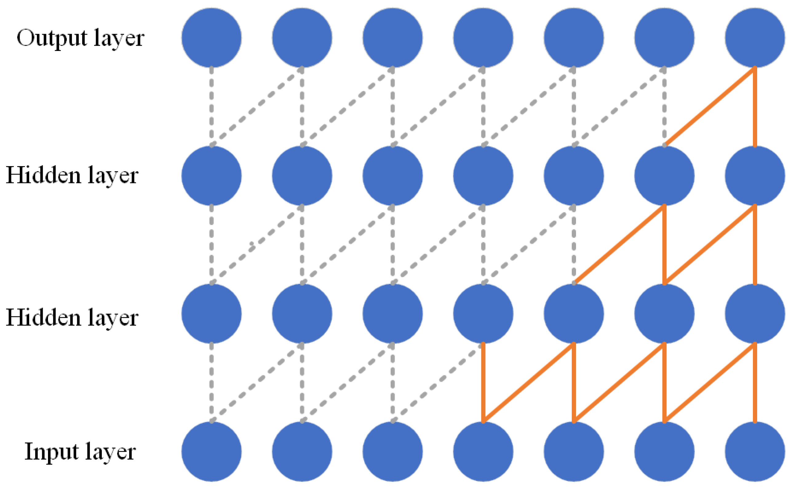
2.1.2. Residual Connection Structure

The extended receptive field depends on the number of hidden layers, and too many hidden layers will cause the gradient to disappear. For this reason, the residual block can avoid this drawback and can be effectively embedded in the TCN structure [31]. According to the essential structure of TCN, each hidden layer contains multiple filters for feature extraction, and the residual block is embedded in the TCN structure; that is, several standard convolutions are replaced. A depth TCN consists of several residual blocks.

To add identity tensors of the same shape, a branch is added to the $1\times 1$ convolution transformation. The output $X^{\left(r\right)}$ of the r-th residual block can be expressed as

$$X^{\left(r\right)}=ReLU(\mathsf{\Gamma }\left(X^{\left(r-1\right)}\right)+X^{\left(r\right)}$$

(2)

in which the activation function uses a rectified linear unit (ReLU). $\mathsf{\Gamma }$ consists of a series of transformations, including dilated causal convolution layer, weight normalization, activation layer and dropout layer. We normalize the weights of the filter and add a dropout after each activation layer for regularization.

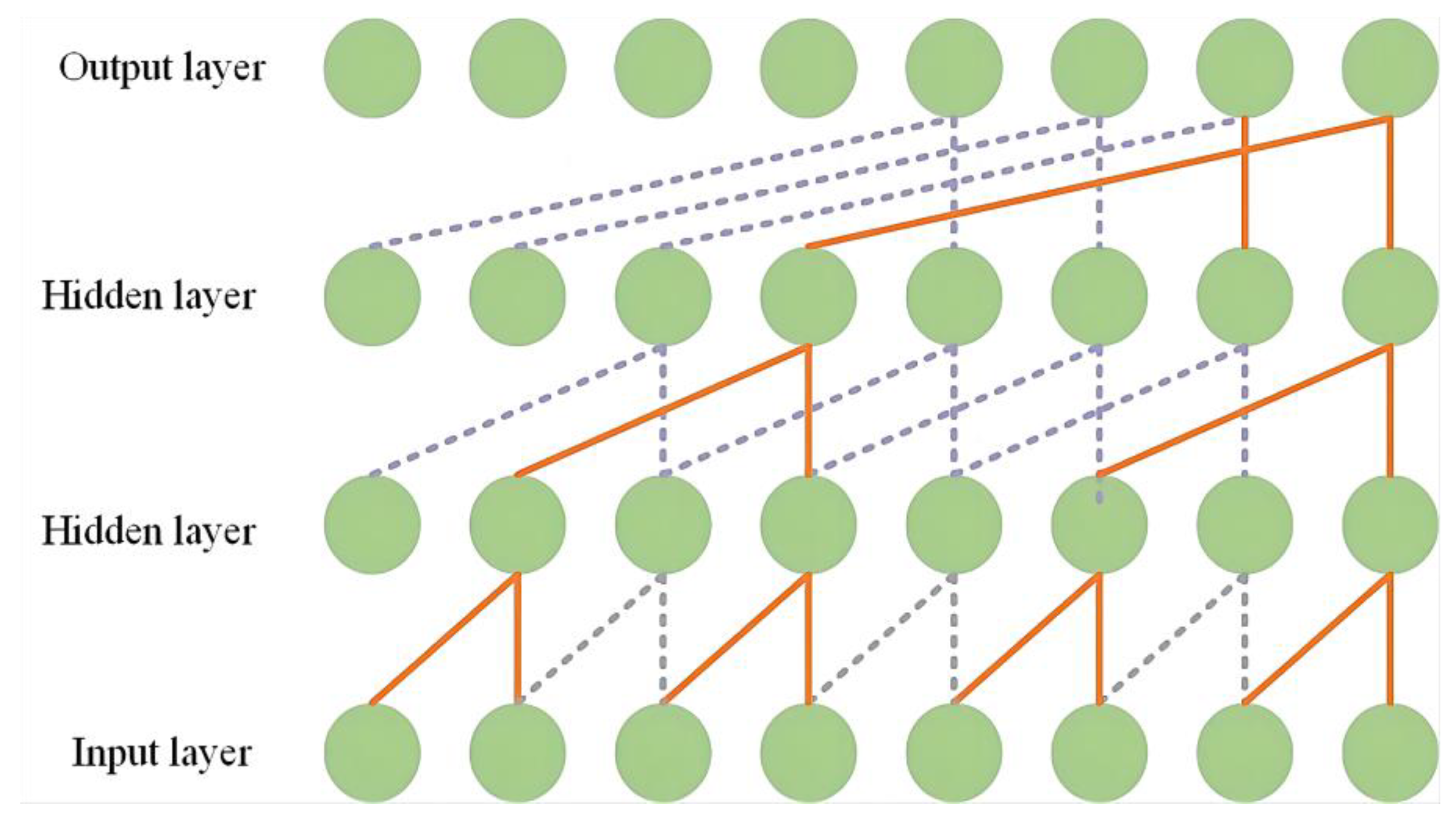
2.1.3. Attention Mechanism

In addition, this paper applies the attention mechanism to the model in TCN. Attention mechanism is the simulation of biological attention, which aims to use algorithms to fit the concerns of characteristic information so as to dynamically adjust the weights of important information and useful information and then suppress and ignore invalid and useless information [32]. The attention weight value of the feature is quantified between 0 and 1, and the final output feature is obtained by adding the product of the attention weight and the feature. The mechanism uses a dynamic loop method. Important features can be highlighted and compared with the original features more effectively in different prediction scenarios. The formula is expressed as follows:

$$z_{ki}=u·\tan h\left(W·h_k+U·h_i+b\right)$$

(3)

$${\alpha }_{ki}=\frac{e^{z_{k_i}}}{{{\displaystyle \sum }}_{j=1}^n{e}^{z_{k_i}}}$$

(4)

$$H={{\displaystyle \sum }}_{i=1}^n{\alpha }_{ki}·h_i$$

(5)

In the formula, $z_{ki}$ represents the measure of feature importance; $u,W$and $U$represent the weight parameter matrix; $b$ denotes the bias; $h_k$ represents the hidden layer status corresponding to the last input; $h_i$ represents the state of the hidden layer corresponding to the i-th element of the input sequence; $\tan h$ is the activation function; ${\alpha }_k$ represents the attention weight of the hidden state of the historical input to the current input; $H$ is the final output characteristic.

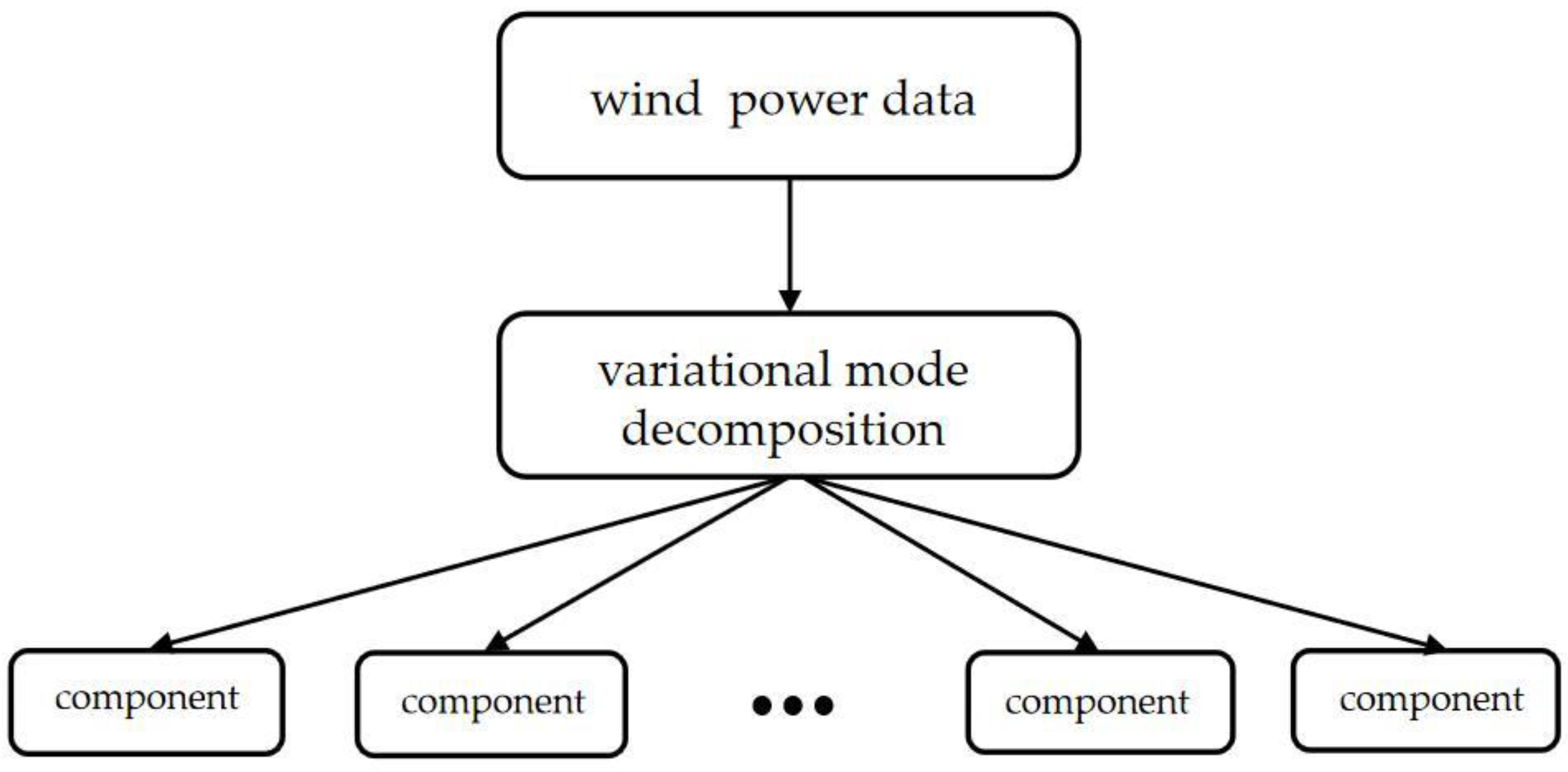
2.2. Variational Mode Decomposition

Variational mode decomposition (VMD) is a non-recursive, adaptive signal processing method that can decompose time series into components with optimal frequency and bandwidth. It overcomes issues of endpoint effects and modal component aliasing in Empirical Mode Decomposition (EMD). See Figure 3 for the VMD process.

The mathematical theory of variable problem can be expressed as:

$$\underset{\left\{y_k\right\},\left\{w_k\right\}}{\min }\left\{{{\displaystyle \sum }}_{k=1}^K\Vert {\partial }_t\left[\left(\left(\delta (t\right)+\frac{j}{nt}\right)\ast y_k\left(t\right)\right]e^{-j{w}_{k}t}{\Vert }_2^2\right\}$$

(6)

Make

$${{\displaystyle \sum }}_k{y}_k=z\left(t\right)$$

(7)

where $y$ represents the set of all patterns; $\left\{y_k\right\}=\left\{y_1,y_2,\cdots ,y_k\right\}$ represents the set of all patterns; $\left\{w_k\right\}=\left\{w_1,w_2,\cdots ,w_k\right\}$ represents the set of respective central frequencies. To solve the constrained variational problem in VMD, we introduce the quadratic penalty $\alpha$ and the Lagrange multiplier $\lambda$ to convert it into an unconstrained problem, as shown in the following formula:

$$\begin{array}{cc}\hfill L\left(\left\{y_k\right\},\left\{w_k\right\},\lambda \right)& =\alpha \{{{\displaystyle \sum }}_{k=1}^K\Vert {\partial }_t\left[\left(\left(\delta (t\right)+\frac{j}{nt}\right)\ast y_k\left(t\right)\right]e^{-j{w}_{k}t}{\Vert }_2^2\hfill \\ & +\Vert z\left(t\right)-{{\displaystyle \sum }}_{k=1}^k{y}_k{\Vert }_2^2\langle \lambda \left(t\right),z\left(t\right)-{{\displaystyle \sum }}_{k=1}^k{y}_k\left(t\right)\rangle \}\hfill \end{array}$$

(8)

Through the application of the alternating direction method of multipliers, the optimal values for $y_k$, $w_k$ and $\lambda$ can be obtained by adjusting the modes and their respective center frequencies. These modes and center frequencies represent the saddle points of unconstrained optimization problems mathematically:

$${\widehat{y}}_k^{n+1}=\frac{\widehat{z}\left(w\right)-{{\displaystyle \sum }}_{i\ne k}{\widehat{y}}_i\left(w\right)+\frac{\widehat{\lambda }\left(w\right)}{2}}{1+2\alpha {\left(w-w_k\right)}^2}$$

(9)

$${\widehat{w}}_k^{n+1}=\frac{{\int }_0^{\infty }w{\left|{\widehat{y}}_k\left(w\right)\right|}^{2}dw}{{\int }_0^{\infty }{\left|{\widehat{y}}_k\left(w\right)\right|}^{2}dw}$$

(10)

$${\widehat{\lambda }}^{n+1}\left(w\right)={\widehat{\lambda }}^n\left(w\right)+\tau (\widehat{z}\left(w\right)-{{\displaystyle \sum }}_k{\widehat{y}}_k^{n+1})$$

(11)

where, $\widehat{z}\left(w\right)$, ${\widehat{y}}_i\left(w\right)$ and $\widehat{\lambda }\left(w\right)$ denote the Fourier transform of each variable, and $n$ is the number of iterations.

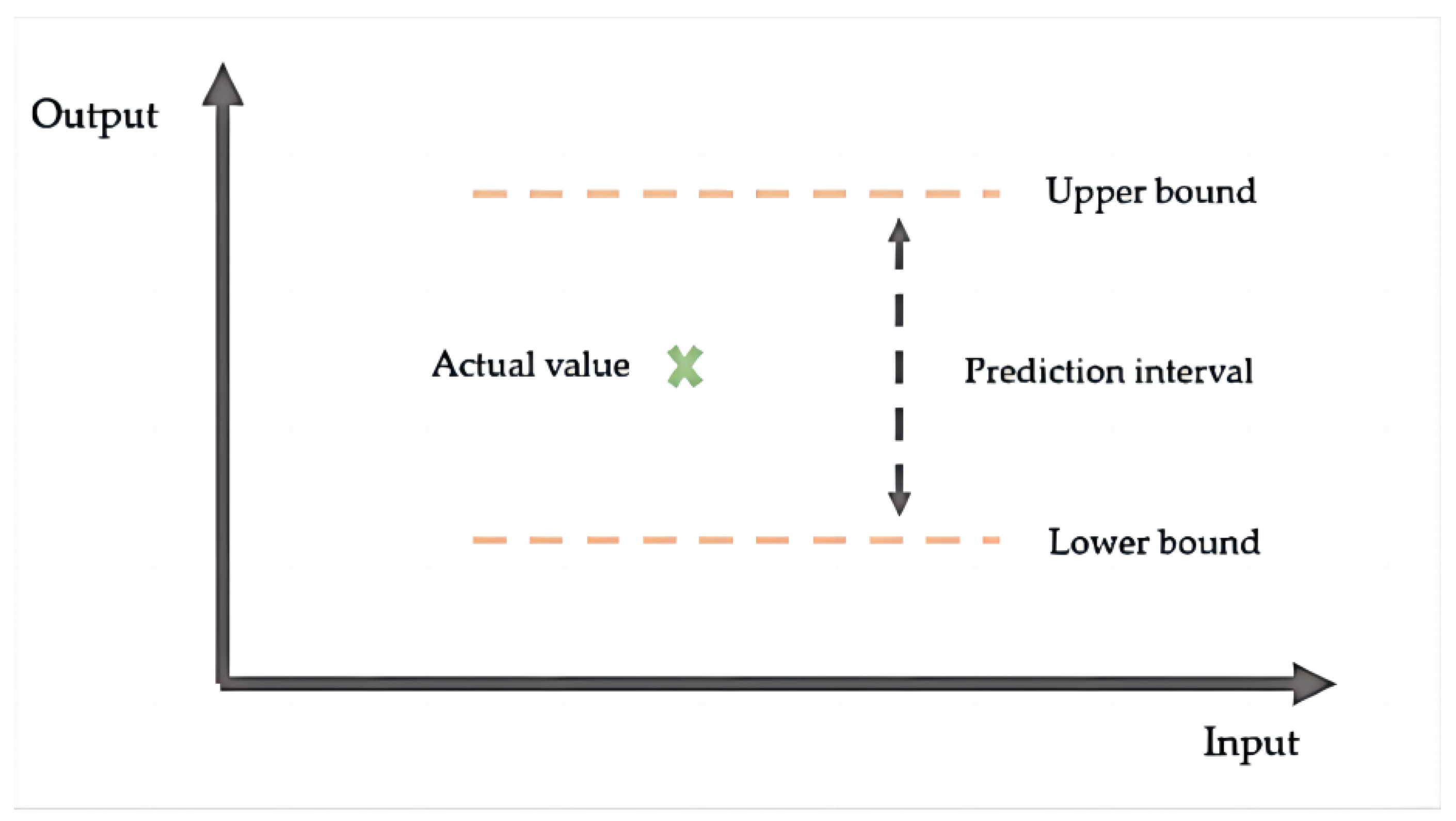
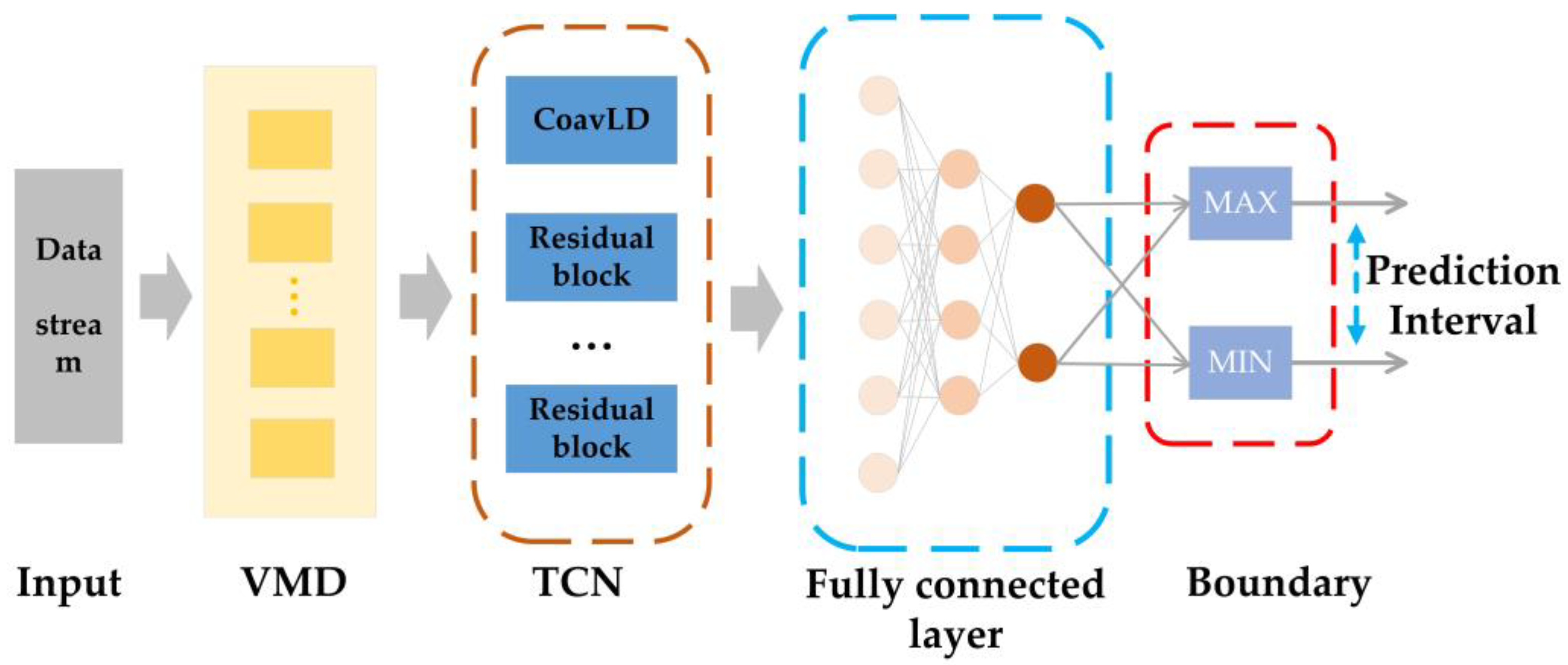
2.3. Interval Prediction Framework

The upper and lower limits of future values are estimated by the prediction interval, as depicted in Figure 4.

Assuming the output error of the linear data-driven model follows a Gaussian distribution with a mean of 0 and a standard deviation of $\sigma$, the upper and lower limits of the model’s output, denoted as $y^U$ and $y^L$, can be established to obtain a prediction interval of $100 \left(1-\alpha \right)\%$, where $\alpha$ is the significance level:

$$y^U=\widehat{y}+Z_{\frac{\alpha }{2\sigma }}$$

(12)

$$y^L=\widehat{y}-Z_{\frac{\alpha }{2\sigma }}$$

(13)

where $Z$ is the standard normal distribution. Since the upper and lower prediction intervals are equivalent, the standard deviation $\sigma$ is equal to the mean square error, commonly known as the predicted mean square error. However, the actual value of standard deviation $\sigma$ is unknown and must be estimated from data. Therefore, it is modified as follows:

$${\sigma }_e^2={{\displaystyle \sum }}_{k=2}^n{\frac{\left(y_k-{\widehat{y}}_k\right)}{n-p}}^2$$

(14)

where $p$ is the number of model parameters. When ${\sigma }_e^2$ is not a constant, the equation becomes more complicated, and it is actually difficult to calculate the value, especially for multivariable or nonlinear models. In the case of nonlinear data-driven prediction models, the mathematical expression can be formulated as

$$y_i=f\left(X_i,{\theta }^{*}\right)+{\xi }_i i=1,2,\cdots ,n$$

(15)

where $X_i$ is the input vector of M-dimensional, and ${\theta }^{*}$ is the best parameter vector of the P-dimensional.${\xi }_i$ is assumed to be independent identically distribution-$N\left(0,{\sigma }^2\right)$.

Suppose that the estimates of $y_i$ and ${\theta }^{*}$ are ${\widehat{y}}_i$ and $\theta$, respectively; then, the Taylor series expansion ignoring the higher order terms is

$${\widehat{y}}_i=c_0+c_1\times \left(\theta -{\theta }^{*}\right) i=1,2,\cdots ,n$$

(16)

$$c_0=f\left(X_i,{\theta }^{*}\right)$$

(17)

$$c_1=\left[\frac{\partial f\left(X_i,{\theta }^{*}\right)}{\partial {\theta }_1} \frac{\partial f\left(X_i,{\theta }^{*}\right)}{\partial {\theta }_2} \cdots \frac{\partial f\left(X_i,{\theta }^{*}\right)}{\partial {\theta }_p}\right]$$

(18)

After the equation is linearized, the prediction limit $100\left(1-\alpha \right)\%$ is established. The upper and lower limits for the model output are

$$y_i^U={\widehat{y}}_i+t_{n-p}^{1-\alpha }s\sqrt{1+c_1{\left(C{C}^{\prime }\right)}^{-1}{c}_1^T}$$

(19)

$$y_i^L={\widehat{y}}_i-t_{n-p}^{1-\alpha }s\sqrt{1+c_1{\left(C{C}^{\prime }\right)}^{-1}{c}_1^T}$$

(20)

where $s$ and $t_{n-p}^{1-\alpha }$ are standard deviation estimation and student-t distribution, and C are the parameters of Jacobian matrix.

It can be seen from the above, in addition to the data distribution constraints, that it is also a problem to calculate the prediction interval of multivariable or nonlinear models with huge amount of calculation and difficulty. The deep learning model is highly valued for its nonlinear modeling and strong learning ability [33]. When it is combined with interval prediction methods, there are considerations of prediction interval coverage probability (PICP) and prediction interval normalized averaged width (PINAW). Wider PINAW can complicate the decision-making process of our prediction results. To obtain a better prediction interval, the observation distribution in the prediction interval can be incorporated into the cost function for adjustment. The study, a new cost function that considers output concentration, PINAW and PICP is proposed, which can be formulated as follows:

$$f\left(PICP,PINAW,CD\right)=W_{PCIP}\times e^{-PICP}+W_{PINAW}\times PINAW+W_{CD}\times CD$$

(21)

where, $W_{PCIP}$ and $W_{PINAW}$ are $W_{CD}$ weight.

The interval prediction model in this paper is shown in Figure 5.

2.4. Evaluation Indicators

The results of the interval prediction and evaluation can be described by interval coverage rate (PICP) and interval average width (PINAW). Among them, under the same prediction interval nominal confidence (PINC), the model performance is better when the PICP value is larger and the PINAW value is smaller. which is defined as

$$PICP=\frac{1}{n}{{\displaystyle \sum }}_{i=1}^n{C}_i$$

(22)

$$C_i=\left\{\begin{array}{c}1 y_i\in \left[L_i,U_i\right]\\ 0 y_i\notin \left[L_i,U_i\right]\end{array}\right\}$$

(23)

$$PINAW=\frac{1}{nR}{{\displaystyle \sum }}_{i=1}^n\left(U_i-L_i\right)$$

(24)

where $n$ is the number of test set samples; $U_i$ and $L_i$ are the generated upper and lower limits of the interval, respectively; $y_i$ is the observed value of the i-th sample; when the observed value is within the interval, it is 1; otherwise, it is 0; R represents the range of the test set, which is used to normalize this index.

In order to comprehensively consider the interval width and coverage, CWC, a comprehensive index based on PICP and PINAW, is introduced as the evaluation standard, and its definition is as follows:

$$CWC=PINAW\left(1+\gamma e^{-\eta \left(PICP-\mu \right)}\right)$$

(25)

$$\gamma =\left\{\begin{array}{c}1 PICP<\mu \\ 0 PICP\ge \mu \end{array}\right\}$$

(26)

where $\mu$ is determined by confidence; $\eta$ is the penalty factor. When the interval coverage is less than the given confidence, an exponential penalty is given; when the coverage is greater than the confidence, only the average interval width PINAW is considered. The smaller the value of the comprehensive index CWC, the better the prediction result.

ERROR describes the deviation between the midpoint of the prediction interval and the actual value, and the formula is as follows:

$$ERROR=\frac{1}{n}{{\displaystyle \sum }}_{i=1}^n\left|\frac{y_i-{\widehat{y}}_i}{{\widehat{y}}_i}\right|\times 100\%$$

(27)

where $n$ is the samples size of test set; $y_i$ is the predicted value of the sample i; ${\widehat{y}}_i$ is the middle of the sample interval.

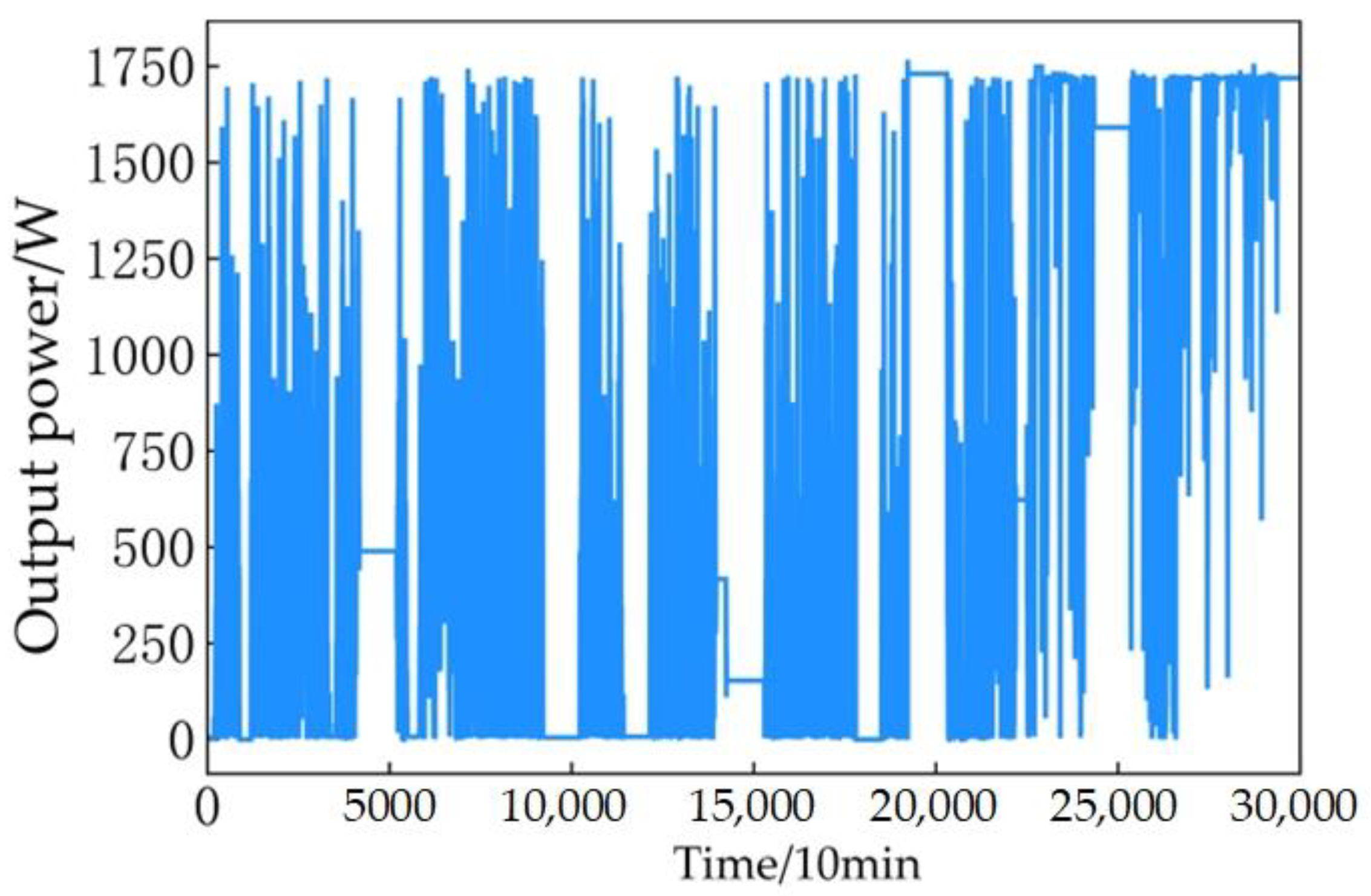
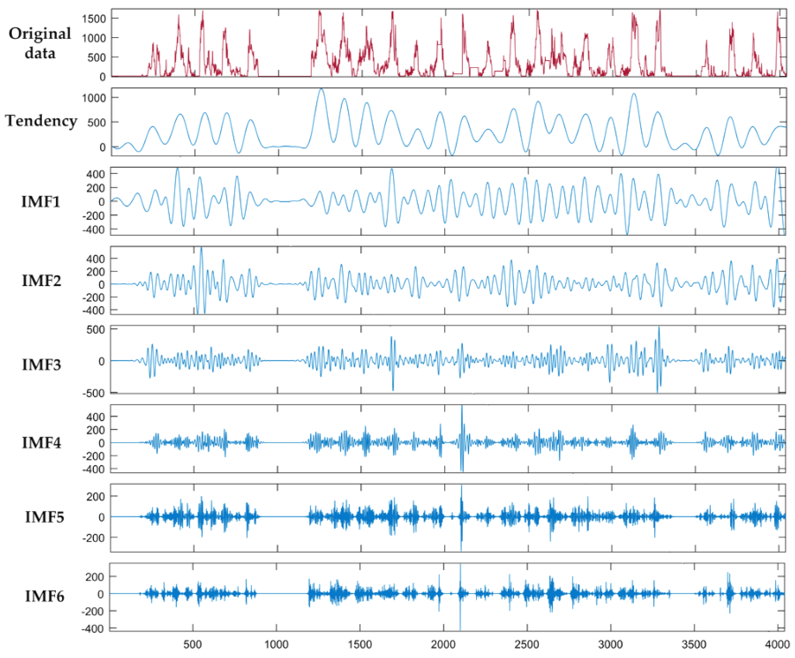
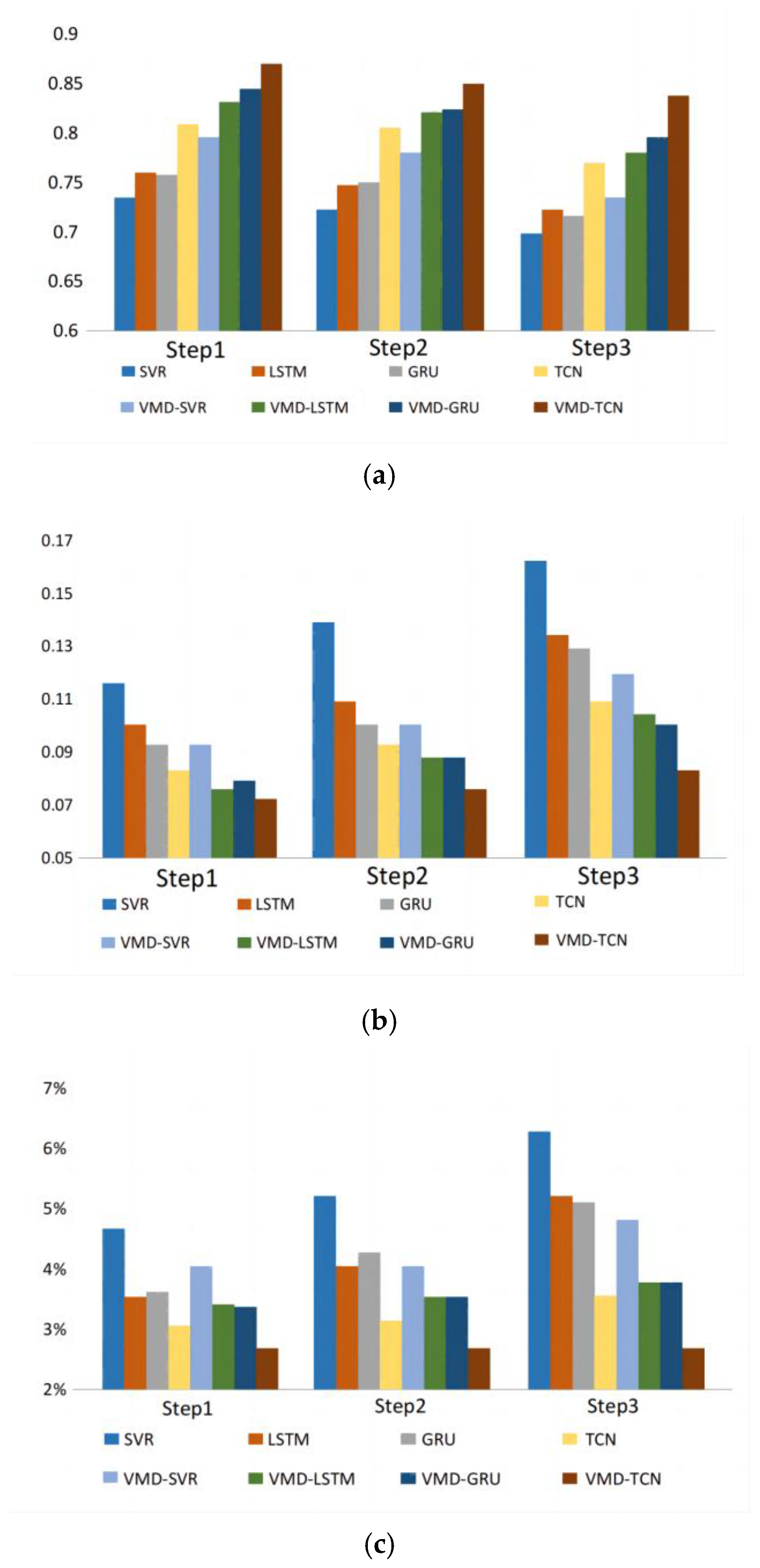
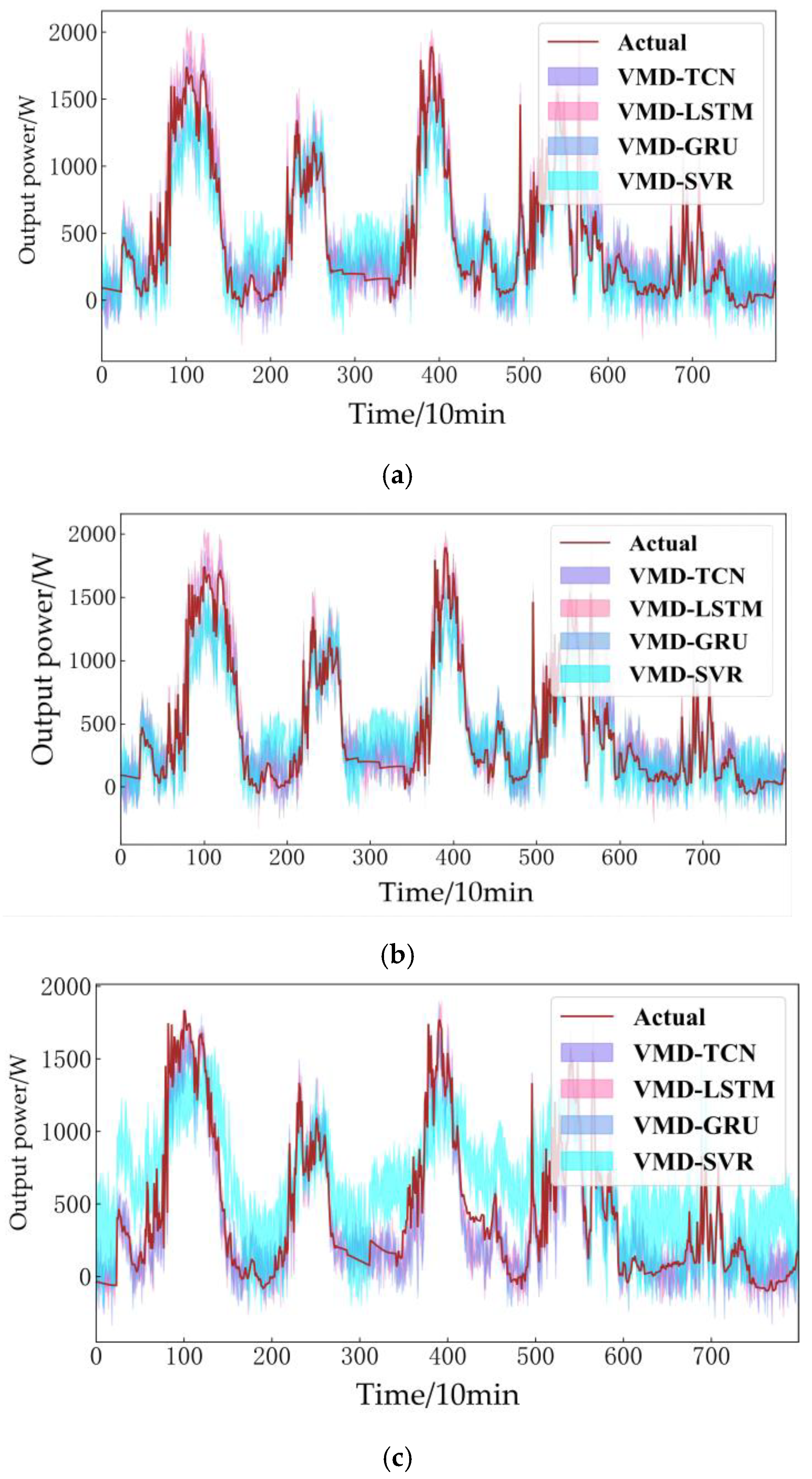
3. Analysis and Discussion

The data used in this paper are wind power data from January 2019 to March 2021, and the sampling frequency is 10 min. The output power data sequence of wind power generation is shown in Figure 6. In order to eliminate the randomness of model training, all experiments were repeated 10 times, and the experimental results were compared and analyzed according to the average values of indicators.

First, variational mode decomposition is used to decompose the acquired wind power generation data. To ensure the fidelity of the signal, the hyperparameter $\alpha$ is 2500 and $\tau$ is 0.35. In order to improve the reliability of the prediction results, divide the sequence more accurately and excavate the characteristics of the sequence. The frequency spectrum analysis method is used to compare the observed signals for many times, and it is found that the signal loss is minimum when decomposed into six components [34]. Therefore, the original signal is decomposed into six component sequences through variational mode decomposition. Figure 7 shows the decomposition results of empirical mode decomposition. In the figure, the original data are divided into two parts: one is the change trend of the main body, and the other is several detailed components.

According to the prior experience, the hyperparameters are set to ensure that the comparison model has relatively consistent complexity. All experimental models run in Python 3.7 compile environment, and the deep learning architecture is based on the Tensorflow2.3 framework. Then, in order to verify the effectiveness and superiority of the proposed model, we compare the predicted results of the proposed model on data sets with other comparable models. In this paper, support vector regression (SVR), long-term and short-term memory neural network (LSTM) and gated cyclic unit neural network (GRU) are selected for comparative analysis. The performance indicators of each model are shown in

Table 1. Performance indicators of each model before and after empirical mode decomposition.

Model	PICP	CWC	ERROR
SVR	0.690	0.123	4.643
LSTM	0.718	0.105	3.656
GRU	0.716	0.099	3.716
TCN	0.768	0.089	2.951
VMD-SVR	0.725	0.098	4.138
VMD-LSTM	0.821	0.081	3.441
VMD-GRU	0.826	0.083	3.413
VMD-TCN	0.882	0.073	2.713

.

Table 1 shows the performance indexes of each model before and after EMD. It can be seen that the VMD-TCN interval prediction model proposed in this paper has achieved good results in PINC, CWC, ERROR and other evaluation indexes. Compared with the comparison model, this method has a significant improvement in performance, higher prediction confidence and narrower prediction interval width. Among the models without empirical mode decomposition, the same TCN has the best performance, while the SVR model has a relatively poor performance. After variational mode decomposition, the comparison shows that the extraction capacity of the TCN is superior to that of the recurring neural networks (LSTM, GRU).

As far as CWC is concerned, VMD-TCN is lower than VMD-SVR, VMD-LSTM and VMD-GRU by 0.025, 0.008 and 0.01, respectively. In ERROR comparison, TCN is lower than SVR, LSTM and GRU by 1.425%, 0.728% and 0.700%, respectively. Among all comparable models, the interval prediction method proposed in this paper combined with variational mode decomposition (VMD) has better extraction ability of TCN, and the final error is reduced to 2.713%.

In addition, by studying the calculation time of all neural network models in the test set, it is found that the TCN model has the fastest load forecasting speed in a single model, and GRU is better than LSTM. When interval prediction is performed, the increased intermediate calculation will undoubtedly increase the operating time of each model [33]. Although the operating time of the VMD-TCN model is more time-consuming than that of the point prediction model, the operating efficiency of the VMD-TCN model is always higher than other models. Although the calculation time of the proposed model is longer than that of the point prediction model, cloud computing and GPU can be used to arrange the model acceleration strategy.

From the observation of Figure 8, it can be seen that the model established in this paper can effectively predict the change trend of wind power generation output power in different step sizes, and the predicted effect is ideal. By comparing TCN and VMD-TCN at the same step length, it is found that the prediction results of VMD-TCN are better than those of TCN, which shows that this decomposition method can effectively reduce the volatility of wind power generation sequence, thus reducing the width of prediction interval and improving the predicted accuracy. Comparing the results of different step sizes, we can find that the prediction performance of each model decreases with the increase in step size. Although the prediction performance of the model proposed in this paper has declined to some extent, its decline is the smallest, and the prediction error is 2.957% even in the third step size.

With the increase in time step, the PICP value of each model decreases in different degrees, because the important information between features may be ignored with the increase in time step, but the PICP of each model is above 0.7, which indicates that each interval prediction model has good confidence. In terms of CWC index, the method proposed by us has obtained the narrowest prediction interval width in almost all cases. Combining all the situations, we conclude that VMD-TCN model performs best.

The VMD-TCN interval prediction model has excellent prediction effect in wind power generation output power, and the TCN network has better performance than the LSTM and GRU neural network. Of course, the optimized VMD-LSTM and VMD-GRU methods also have the potential to improve the prediction effect. It can be seen that the prediction results of each interval model through empirical mode decomposition are shown in Figure 9, and the results in the figure also confirm the feasibility of the prediction.

4. Conclusions

In this article, based on empirical mode decomposition and the time convolution network method, wind power interval prediction is modeled to efficiently predict short-time wind power output data series. First, empirical mode decomposition is used to eliminate the non-stationary features of the original data flow. Then, the interval prediction framework of upper and lower limit estimation is introduced, and the time convolution network interval prediction model is used to further mine the prediction results of wind power generation. The third chapter of the data analysis of previous years found that the model has good prediction performance at different step sizes, indicating that the model has high stability. After empirical mode decomposition, the prediction interval of each model is more stable; on the premise that PINC meets the confidence level, the prediction interval width obtained by VMD-TCN is narrower.

In addition to the above performance, we should not ignore the influence of weather data and high-dimensional data characteristics on the performance of the prediction model. Therefore, in the future work, it is still the focus of the new load data forecasting task to study the forecasting effect of related factors and verify the effect in different scenarios and explore ways to improve the accuracy of forecasting model and data preprocessing.

References

1. Zhou, M.; Huang, Y.; Li, G. Changes in the concentration of air pollutants before and after the COVID-19 blockade period and their correlation with vegetation coverage. Environ. Sci. Pollut. Res. Int. 2021, 28, 23405–23419. [Google Scholar] [CrossRef] [PubMed]
2. Xiao, G.; Xiao, Y.; Ni, A.; Zhang, C.; Zong, F. Exploring influence mechanism of bike sharing on the use of public transportation-a case of Shanghai. Transp. Lett. Int. J. Transp. Res. 2022, 1–9. [Google Scholar] [CrossRef]
3. Wan, C.; Song, Y. Theories, Methodologies and Applications of Probabilistic Forecasting for Power Systems with Renewable Energy Sources. Autom. Electr. Power Syst. 2021, 45, 2–16. [Google Scholar]
4. Huang, Y.; Zhou, N.; Zhang, S.; Yang, X.; Zhang, S.; Liu, H. Research on PV Power Forecasting Based on Wavelet Decomposition and Temporal Convolutional Networks. In Proceedings of the 2021 IEEE 4th International Electrical and Energy Conference (CIEEC), Wuhan, China, 28–30 May 2021; pp. 1–6. [Google Scholar]
5. Pullanagari, R.R.; Kereszturi, G.; Yule, I.J.; Irwin, M. Determining Uncertainty Prediction Map of Copper Concentration in Pasture from Hyperspectral Data Using Quantile Regression Forest. In Proceedings of the IGARSS 2018—2018 IEEE International Geoscience and Remote Sensing Symposium, Valencia, Spain, 22–27 July 2018; pp. 3809–3811. [Google Scholar]
6. Yang, X.Y.; Zhang, Y.F.; Ye, T.Z. Prediction of Combination Probability Interval of Wind Power Based on Naive Bayes. High Volt. Technol. 2020, 46, 1099–1108. [Google Scholar]
7. Xiao, G.; Cui, W. Evolutionary game between government and shipping companies based on shipping cycle and carbon quota. Front. Mar. Sci. 2023, 10, 11321. [Google Scholar] [CrossRef]
8. Yang, X.Y.; Xing, G.; Ma, X. A model of quantile regression with kernel extreme learning machine and wind power interval prediction. Sol. Energy 2020, 41, 300–306. [Google Scholar]
9. Yan, J.; Li, K.; Bai, E.-W.; Deng, J.; Foley, A.M. Hybrid probabilistic wind power forecasting using temporally local gaussian process. IEEE Trans. Sustain. Energy 2015, 7, 87–95. [Google Scholar] [CrossRef] [Green Version]
10. Gan, Z.; Li, C.; Zhou, J.; Tang, G. Temporal convolutional networks interval prediction model for wind speed forecasting. Electr. Power Syst. Res. 2021, 191, 106865. [Google Scholar] [CrossRef]
11. Chen, X.; Liu, S.; Liu, R.W.; Wu, H.; Han, B.; Zhao, J. Quantifying Arctic oil spilling event risk by integrating an analytic network process and a fuzzy comprehensive evaluation model. Ocean Coast. Manag. 2022, 228, 106326. [Google Scholar] [CrossRef]
12. Khosravi, A.; Nahavandi, S.; Creighton, D.; Atiya, A.F. Lower upper bound estimation method for construction of neural network-based prediction intervals. IEEE Trans. Neural Netw. 2010, 22, 337–346. [Google Scholar] [CrossRef]
13. Shrivastava, N.A.; Khosravi, A.; Panigrahi, B.K. Prediction interval estimation of electricity prices using PSO tuned support vector machines. IEEE Trans. Ind. Inf. 2015, 11, 322–331. [Google Scholar] [CrossRef]
14. Viet, D.T.; Phuong, V.V.; Duong, M.Q.; Tran, Q.T. Models for Short-Term Wind Power Forecasting Based on Improved Artificial Neural Network Using Particle Swarm Optimization and Genetic Algorithms. Energies 2020, 13, 2873. [Google Scholar] [CrossRef]
15. Zhang, C.; Wei, H.; Xie, L. Direct interval forecasting of wind speed using radial basis function neural networks in a multi-objective optimization framework. Neurocomputing 2016, 205, 53–63. [Google Scholar] [CrossRef]
16. Liu, X.; Qiu, L.; Rodriguez, J.; Wang, K.; Li, Y.; Fang, Y. Learning-Based Neural Dynamic Surface Predictive Control for MMC. IEEE Trans. Power Electron. 2023, 38, 53–59. [Google Scholar] [CrossRef]
17. Liu, X.; Qiu, L.; Fang, Y.; Rodriguez, J. Reinforcement Learning-Based Event-Triggered FCS-MPC for Power Converters. IEEE Trans. Ind. Electron. 2023, 1–12. [Google Scholar] [CrossRef]
18. Mhaskar, H.; Liao, Q.; Poggio, T. Learning functions: When is deep better than shallow. arXiv 2016, arXiv:1603.00988. [Google Scholar]
19. Huang, Y.; Zhou, M.; Yang, X. Ultra-short-term photovoltaic power forecasting of multi-feature based on hybrid deep learning. Int. J. Energy Res. 2022, 46, 1370–1386. [Google Scholar] [CrossRef]
20. Zhou, M.; Huang, Y.; Yang, H. Temperature forecast based on integration of GRU neural network and Grey model. J. Trop. Meteorol. 2020, 36, 855–864. [Google Scholar]
21. Aly, H.H. A novel deep learning intelligent clustered hybrid models for wind speed and power forecasting. Energy 2020, 213, 118773. [Google Scholar] [CrossRef]
22. Quan, H.; Srinivasan, D.; Khosravi, A. Short-term load and wind power forecasting using neural network-based prediction intervals. IEEE Trans. Neural Netw. 2014, 25, 305–315. [Google Scholar] [CrossRef]
23. Kavousi-Fard, A.; Khosravi, A.; Nahavandi, S. A new fuzzy-based combined prediction interval for wind power forecasting. IEEE Trans. Power Syst. 2015, 31, 18–26. [Google Scholar] [CrossRef]
24. Tahmasebifar, R.; Moghaddam, M.P.; Sheikh-El-Eslami, M.K.; Kheirollahi, R. A new hybrid model for point and probabilistic forecasting of wind power. Energy 2020, 211, 119016. [Google Scholar] [CrossRef]
25. Korprasertsak, N.; Leephakpreeda, T. Robust short-term prediction of wind power generation under uncertainty via statistical interpretation of multiple forecasting models. Energy 2019, 180, 387–397. [Google Scholar] [CrossRef]
26. Li, C.; Tang, G.; Xue, X. Short-term wind speed interval prediction based on ensemble GRU model. IEEE Trans. Sustain. Energy 2020, 11, 1370–1380. [Google Scholar] [CrossRef]
27. Khodayar, M.; Wang, J. Spatiotemporal graph deep neural network for short-term wind speed forecasting. IEEE Trans. Sustain. Energy 2019, 10, 670–681. [Google Scholar] [CrossRef]
28. Bai, S.; Kolter, J.Z.; Koltun, V. An empirical evaluation of generic convolutional and recurrent networks for sequence modeling. arXiv 2018, arXiv:1803.01271. [Google Scholar]
29. Wan, R.; Mei, S.; Wang, J. Multivariate temporal convolutional network: A deep neural networks approach for multivariate time series forecasting. Electronics 2019, 8, 876. [Google Scholar] [CrossRef] [Green Version]
30. Zhang, Z.; Wang, X.; Jung, C. DCSR: Dilated convolutions for single image super-resolution. IEEE Trans. Image Process. 2019, 28, 1625–1635. [Google Scholar] [CrossRef]
31. Zhang, K.; Sun, M.; Han, T.X. Residual networks of residual networks: Multilevel residual networks. IEEE Trans. Circuits Syst. Video Technol. 2018, 28, 1303–1314. [Google Scholar] [CrossRef] [Green Version]
32. Vaswani, A.; Shazeer, N.; Parmar, N. Attention is all you need. In Proceedings of the Advances in Neural Information Processing Systems 30: Annual Conference on Neural Information Processing Systems, Long Beach, CA, USA, 4–9 December 2017; pp. 5998–6008. [Google Scholar]
33. Chen, X.; Wu, S.; Shi, C.; Huang, Y.; Yang, Y.; Ke, R.; Zhao, J. Sensing Data Supported Traffic Flow Prediction via Denoising Schemes and ANN: A Comparison. IEEE Sens. J. 2020, 20, 14317–14328. [Google Scholar] [CrossRef]
34. Zheng, J. Experimental study of IMF component determination Criterion Method in empirical mode decomposition. Geomat. Geogr. Inf. Technol. 2021, 46, 33–37. [Google Scholar] [CrossRef]
Figure 1. Causal convolution structure.
Sustainability 15 06114 g001
Figure 2. Dilated convolutional architecture.
Sustainability 15 06114 g002
Figure 3. Variational mode decomposition implementation process.
Sustainability 15 06114 g003
Figure 4. The upper and lower bounds of the prediction interval.
Sustainability 15 06114 g004
Figure 5. Overall design architecture of interval prediction model.
Sustainability 15 06114 g005
Figure 6. Wind power data series.
Sustainability 15 06114 g006
Figure 7. Variational mode decomposition results of wind power data.
Sustainability 15 06114 g007
Figure 8. Performance indicators of different models with varying step sizes. (a) Interval coverage; (b) Coverage width standard; (c) Error.
Sustainability 15 06114 g008
Figure 9. Prediction results of different models with varying step sizes. (a) Step I; (b) Step II; (c) Step III.
Sustainability 15 06114 g009