Distributed Traffic Control Based on Road Network Partitioning Using Normalization Algorithm

Abstract

With continuous economic development, most urban road networks are facing unprecedented traffic congestion. Centralized traffic control is difficult to achieve, and distributed traffic control based on partitioning a road network into subnetworks is a promising way to alleviate traffic pressure on urban roads. In order to study the differences between different partitioning methods chosen for distributed traffic control, we used the normalization algorithm to partition a part of the road network in Changsha City, and we used the results of the Girvan–Newman algorithm and the manual empirical partitioning method as a control group. Meanwhile, an abstract road network was constructed using VISSIM simulation software based on realistic road network parameters. And then, the different partitioning results were applied to the simulated road network to analyze the control effect. The results of the simulation software show that different partitioning methods have different effects on traffic control at subnetwork boundaries and improve traffic pressure to different degrees. Partitioning the road network into four subnetworks provided the greatest degree of traffic improvement. Overall, the proposed distributed traffic control method effectively improved operational efficiency and alleviated the traffic pressure of the road network.

1. Introduction

In early urban planning, urban road design usually focused on practical needs and lacked long-term consideration based on the small number of vehicles that were initially present. With an increasing number of vehicles on roads, traffic has increased, and some urban roads are overwhelmed [1]. And the increase in traffic will also have an impact on driving safety. Under these conditions, increasing the width of roads is a long-term solution for increasing their capacity and improving traffic congestion. However, increasing the width of a road involves a long construction period and wide range of considerations. Although increasing the width of roads can alleviate traffic pressure, unbalanced traffic pressure on urban roads is also a major factor limiting the operation efficiency of road networks [2]. Traffic congestion during peak periods can lead to aggressive driving behaviors associated with crash risk. As roads become congested, drivers’ response patterns will become more aggressive. And when drivers leave congested roads, they pay more attention to driving safety [3]. Therefore, equalizing traffic pressure is important for driving safety. During peak hours, urban expressways and arterial roads are congested, whereas secondary arterial roads and branch roads flow smoothly. Using smoothly flowing secondary arterial roads and branch roads to optimize the control of congested expressways and arterial roads can provide a rapid and stable solution for alleviating local congestion [4]. It can also reduce the possibility of traffic accidents [3]. As congestion on expressways and main roads is relieved, the probability of traffic accidents decreases. For otherwise clear secondary and branch roads, the number of vehicles being diverted to these roads is not sufficient to cause traffic congestion. However, the increase in traffic flow increases the likelihood of traffic conflicts [5]. Some studies have shown that there is a significant correlation between the number of traffic conflicts and the number of traffic accidents [6,7]. Therefore, when using secondary and branch roads to relieve congestion on expressways and trunk roads, it is necessary to strengthen safety control on the diverted roads at the same time to avoid traffic accidents due to the increased traffic volume.

In addition, a detailed and efficient control strategy is required to achieve a balanced effect on the road network. However, an urban road network typically involves hundreds of signaled intersections, and centralized control of these signals is difficult. Distributed control can effectively alleviate this problem [8]. Distributed control entails partitioning of a large road network into regional subnetworks using a clustering method and then applying control within each subnetwork and at the boundaries between subnetworks [9]. This method realizes the signal control of large road networks while reducing computational complexity [4]. Additionally, control at regional boundaries does not depend on the current state of the road network, and controlling the traffic flow in the network does not require assumptions regarding parameters that are difficult to observe [10].

When a road network is divided into subnetworks with small variations in traffic density, the macroscopic fundamental diagrams (MFDs) of subnetworks have more homogeneous distributions, which reduces interference with network traffic flow control [11,12]. Additionally, the homogeneous spatial distribution of traffic density in individual subnetworks makes it more feasible to control traffic flow at the boundaries between subnetworks [13,14,15]. Partitioning a heterogeneous road network into homogeneous subnetworks with low variations in traffic density ensures that each subnetwork has a single clear MFD, which facilitates coordination between subnetworks [10]. Several methods (Zheng et al. (2020); Li and Gong (2006); Potuzak (2013)) are available for network partitioning. At the core of these methods is the definition of reasonable criteria for partitioning [16,17,18]. The major criterion for road network partitioning is the association between intersections, which considers the static structural characteristics and dynamic traffic parameters of intersections [19]. Highly associated intersections are clustered in the same subnetwork to facilitate optimal control strategies [15,20]. Zhou et al. [21] proposed a fast Newman algorithm-based method for traffic network partitioning and applied it to the partitioning of a large road network. However, their method yielded subnetworks with widely varying scales. Lu et al. [22] proposed equations for computing the association between pairs of adjacent intersections and the combined association between multiple intersections, and they developed a partitioning model for the control of subnetworks. However, their method has high time complexity, making it infeasible for application to real large road networks. Zhou et al. [23] suggested that traffic control of a large urban road network necessitates partitioning into subnetworks and that a control algorithm should be both effective at extracting subnetwork information and fast at performing computations. They proposed a method for calculating the demand for connection between pairs of adjacent intersections. Based on this method, the weights of individual road sections were calculated and used as criteria for network partitioning.

Ji et al. [24] proposed an MFD-based method for traffic control network partitioning that partitions a road network based largely on the features of congestion in specific time periods. Ma et al. [25] and Yin et al. [26] proposed spectral methods for the partitioning of traffic networks based on the association between pairs of adjacent intersections. Li et al. [27] applied macro-traffic flow theory to traffic network partitioning and proposed a traffic network partitioning method based on the traffic density on individual roads. However, most existing methods for traffic network partitioning are based on historical or simulation data of small road networks. Therefore, their applicability to real large road networks is questionable. Additionally, the objectives and principles of partitioning are not clearly defined [28]. For large road networks, subnetwork partitioning must take into account the correlation of roads within a subnetwork and the variation between subnetworks. Choosing an overly microscopic approach may result in the inclusion within a subnetwork of isolated road segments that belong to other subnetworks. Such partitioning results are not conducive to the application of traffic control strategies. In addition, isolated road segments may affect the control effect. Therefore, algorithms that focus more on the macro level need to be selected when performing area delineation. The normalization algorithm, as a partitioning method in graph theory, focuses on the overall characteristics of the graph, so it does not produce isolated road segments and is suitable for subnetwork partitioning of large road networks. Therefore, the normalization algorithm was adopted for traffic network partitioning in this study.

Several studies (Xu (2019); Huang (2020); Arenas et al. (2004); Widinson and Huberman (2004); Lin et al. (2016); and Shen and Wu (2017)) have shown that dynamic feedback-based control of the traffic flow at the boundaries between subnetworks facilitates better balancing of the traffic flow across an entire network [4,29,30,31,32,33]. For large traffic networks consisting of multiple regional subnetworks, the strategy for controlling traffic at the boundaries between subnetworks is complex [34]. First, the quality of road network partitioning must be considered because the resulting road subnetworks directly affect the stability of MFDs, thereby affecting the control of the entire network [35,36,37]. Demonstrating the effectiveness of the normalization algorithm for road network partitioning requires comparisons to another partitioning algorithm.

Urban traffic networks are discrete, strongly coupled, and nonlinear complex networks. Complex network theory is often used to investigate urban traffic networks [16,38,39]. The intersections in a traffic network are represented as nodes in a complex network, road sections are represented as edges, and the attributes of road sections are represented as the weights of edges. In this manner, the urban traffic network partitioning problem can be abstracted as the community partition problem in complex weighted networks. The Girvan–Newman (GN) algorithm is a community detection algorithm that is simple in theory, can accurately detect small community structures, and is very suitable for road network partitioning. This method is chosen as a control for the normalization algorithm, which can achieve both fast identification of subnetworks and reduced computational difficulty. At the same time, the normalization algorithm and the GN algorithm belong to two parts of the theories of graph theory and complex networks, respectively, and their comparison better reflects the variance of different partitioning methods. Therefore, the GN and normalization algorithms were compared in this study to investigate the effects of different partitioning methods on the network-partitioning-based traffic control of road networks. In order to more clearly show that the road network classification based on real data is more objective and effective, the experience-based manual method is also selected as a control group in this paper. It is mainly based on several factors such as road class, number of lanes, and historical congestion to determine the result of area classification.

From the above scholars’ research, it is clear that for large-scale urban road networks partitioning the city into several subnetworks for control can effectively reduce the control difficulty. At the same time, the control of subnetwork boundaries can not only connect adjacent subnetworks, but also reduce the influence of traffic dynamics on the control. The relationship between the partitioning method and the control effect is still unclear. Therefore, in order to explore the influence of different partitioning methods on the coordination control results, this paper takes part of the Changsha City road network as the research object, and it selects the normalization algorithm and GN algorithm as the partitioning algorithms to study the coordination control effect on the simulated road network.

2. Literature Review

The concept of subnetwork traffic control [40] was introduced in the 1970s. Since different areas in a city have different functions, the plans for the road networks are different, and the operational conditions of the traffic flow may vary. Therefore, when studying the traffic characteristics of road networks, it is necessary to first develop certain criteria. According to these criteria, appropriate algorithms are applied to road sections with similar characteristics in a complex and large road network. A heterogeneous road network is divided into several homogeneous subnetworks so that the corresponding control optimization scheme can be implemented according to the traffic flow characteristics of each cell.

There have been some studies on urban road network subnetwork classification algorithms that consider the static characteristics of road network subnetworks [41]. For example, Geroliminis et al. [35] analyzed the historical traffic flow data of road networks, used density to measure the similarity between road segments, and introduced the idea of image segmentation to subnetwork road segments in road networks. Mohammadreza et al. [42] proposed a three-step clustering algorithm to divide heterogeneous networks into connected homogeneous regions. Yan et al. [43] defined a similarity model based on link autocorrelation analysis and established a static partitioning framework to divide large heterogeneous traffic networks into several homogeneous subregions by analyzing the spatiotemporal similarity and spatial heterogeneity of link characteristics. Ji et al. [44] used the concept of maximum connected component (MCC) to describe the heterogeneous networks as several homogeneous subnetworks to visualize the evolution of congestion.

In the study of traffic control subnetworks, static classification is mainly based on the traffic organization form of the road network. With the increasing number of motor vehicles, scholars began to study how to incorporate the dynamics of the traffic road network into the subnetwork classification algorithm in order to meet the demand of dynamic changes in traffic [45,46,47,48].

Qin [49] used simulation data to measure the temporal-spatial similarity of road operations in terms of road section density throughout the day and proposed a local road network subnetwork partitioning algorithm based on a macro fundamental diagram and spectral clustering algorithm. Wagner et al. [45] developed two heuristic partitioning algorithms to find traffic subnetworks with uniform traffic levels using a defined mixed integer linear optimization model. Dong et al. [50] combined the traffic dynamic characteristics of the road network, proposed a traffic subnetwork partitioning model based on the MFD theory, and proposed a key control zone identification method. Hu et al. [51] established a correlation degree model for quantitative correlation between adjacent intersections of arterial roads based on traffic state data, and they selected a density-based spatial clustering application and a noise algorithm to cluster the derived indices to achieve control subnetwork partitioning of arterial roads. Xu et al. [52] proposed a dynamic partitioning method for road networks based on the different degrees of congestion for intersections with different states in the road network, considering the correlation of intersections within the subnetwork. Sun [53] analyzed the characteristics and applicability of three models, the Whitson model, the Whitson improvement model, and the path correlation degree model; selected local road networks; and calculated the correlation degree using the three models. According to the traffic demand and correlation degree, the traffic flow characteristics of the road network and the path and turning ratio of the road network were combined. Finally, the hierarchical clustering method was applied to classify the subnetworks.

In summary, in terms of traffic subnetwork delineation algorithms, they can be divided into two categories: static algorithms and dynamic algorithms. Static methods, which are mainly based on the geographic set characteristics of the road network for traffic subnetwork delineation, ignore the dynamic characteristics of the traffic system and cannot accurately reflect the importance of various factors in the subnetwork delineation process. The dynamic method, considering the dynamic characteristics of traffic flow in the urban road network, divides subnetworks according to the correlation of traffic flow between spatial and temporal dimensions. The main algorithms of dynamic methods include clustering algorithms and heuristic algorithms. Although the heuristic algorithm can still perform subnetwork classification with a certain amount of missing data, it can often only obtain the locally optimal subnetwork classification result, which has a large deviation from the actual subnetwork. The clustering algorithm, on the other hand, has high efficiency of operation, and at the same time, can better achieve the global optimal result by combining with the optimization objective. The classification results will be affected by the algorithm, so it is necessary to choose a suitable classification algorithm by combining the road network data and optimization requirements.

3. Basic Data and Traffic Simulation

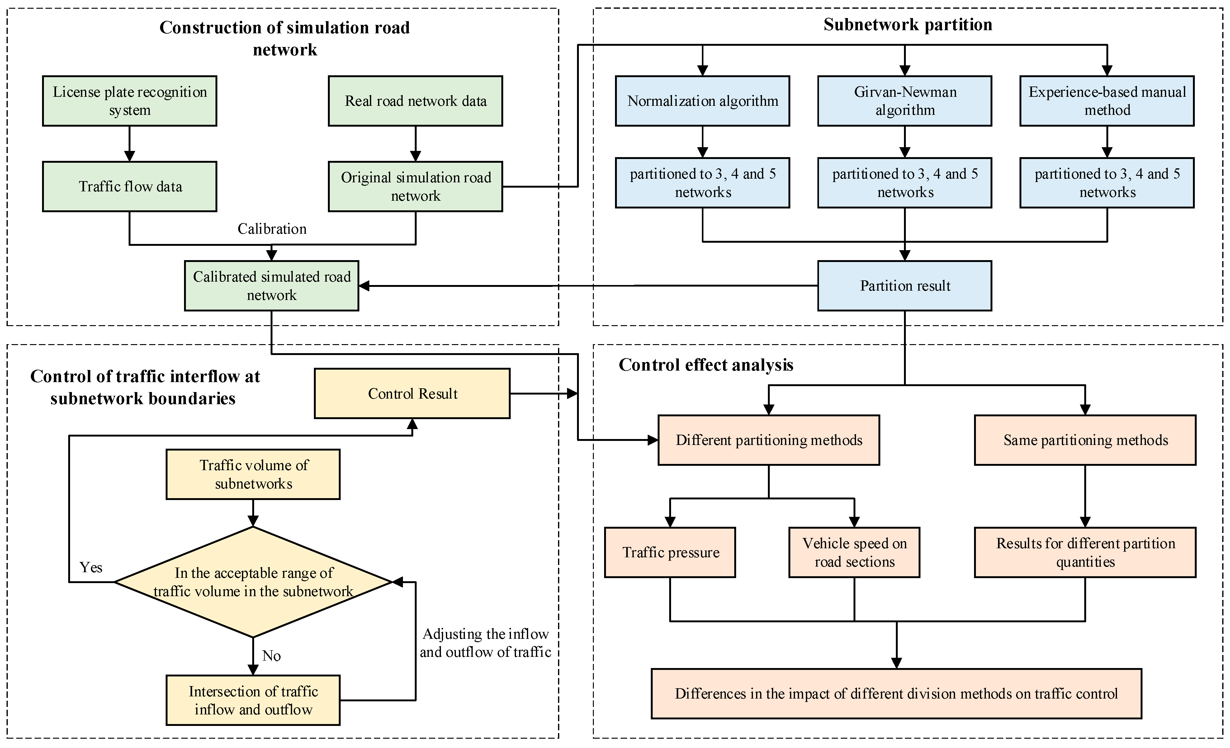
The research in this paper includes four main aspects, namely, the construction of the simulation road network, the partitioning of subnetworks, the control of traffic flow at subnetwork boundaries, and the analysis of the control effect. The research flow chart is shown in Figure 1.

As can be seen from the flow chart, we first needed to build and calibrate the simulated road network according to the real road network parameters and the traffic data collected via license plate recognition system. And then, the simulated road network was partitioned into 3, 4, and 5 subnetworks by using three division methods. In this process, the input parameters and evaluation indices of the road network were kept constant. For the subnetworks, traffic control was performed by first determining whether the traffic flow within the subregion met the acceptable range. If it was within the acceptable range, optimal control could be performed. If it was not within the acceptable range, it was necessary to adjust the traffic flow of the subnetwork via flow inflow and outflow intersections. After the control period was simulated is completed, the control results were analyzed. For the same partitioning method, we needed to compare the differences in the number of different partition categories. For different partitioning methods, we needed to compare the differences in traffic pressure and road speed of the road network.

3.1. Study Area

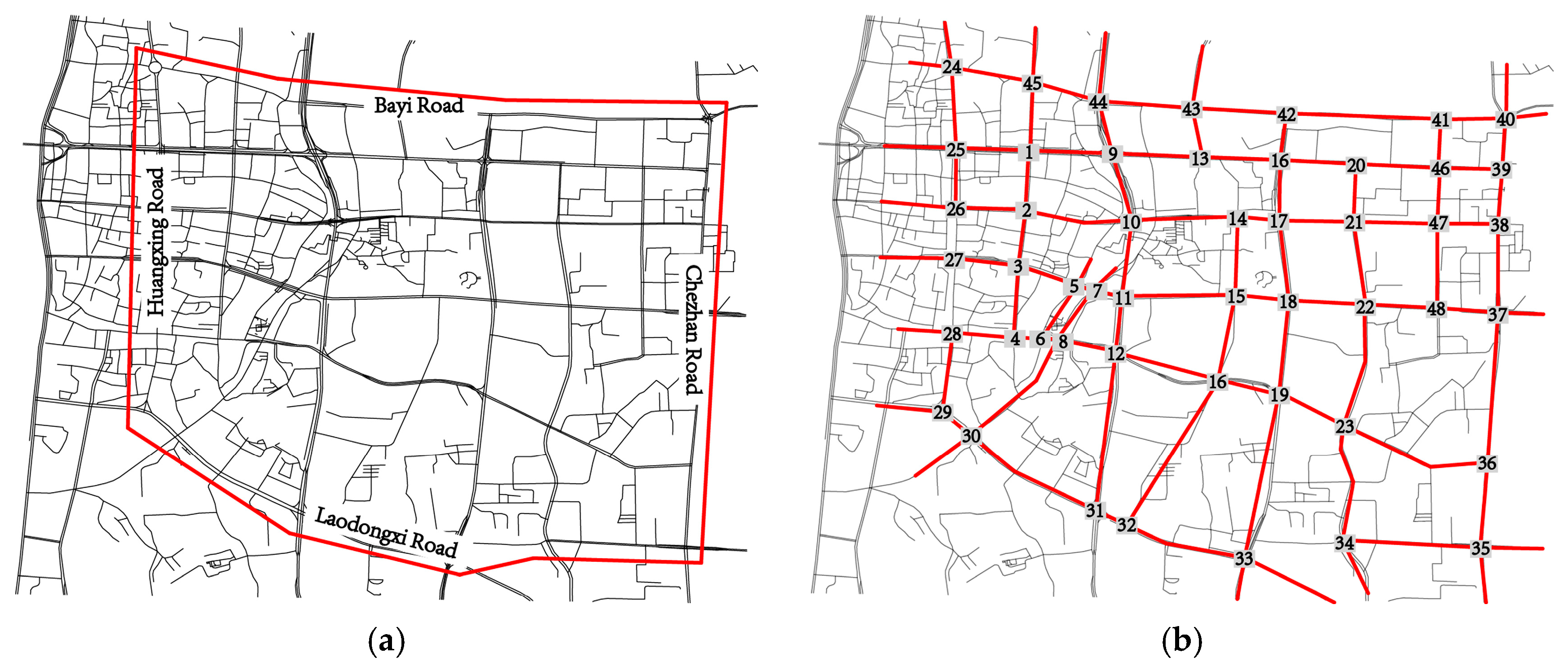
A part of the road network in Changsha City (Figure 2a) was selected as the target network for this study. The study area extends from the Bayi Road in the north to Laodongxi Road in the south and from the Huang Xing Road in the west to the Chezhan Road in the east. The network consists of several arterial roads, secondary arterial roads, and branch roads. To ensure the accuracy of the traffic information from the network, the network was abstracted based on location from the license plate recognition system from Changsha City (Figure 2b). The network contains 48 intersections. The numbers in the map represent intersection numbers.

3.2. Data Description

As this study focused on the effects of network-partitioning-based distributed traffic control on road network traffic congestion, the traffic conditions of the road network during morning and evening peak hours on weekdays were investigated. During morning peak hours, the road network experiences severe traffic congestion on most road sections. Despite the network containing two-way eight-lane and two-way ten-lane roads, traffic pressure is significant with many areas of local congestion. Based on traffic data collected via license plate recognition system, vehicle traffic from five consecutive weekdays (1–5 July 2019) was analyzed. The traffic distributions during morning peak hours (7:00 to 9: 00 a.m.) on the five weekdays exhibit similar trends. The vehicle traffic data were averaged for subsequent analyses.

Table 1. Basic traffic information at representative intersections.

Serial Number of Intersection	Direction of Incoming Road	Number of Lanes of Incoming Road	Length of Incoming Road (m)	Traffic Flow of Incoming Road (Vehicles/h)	Serial Number of Intersection	Direction of Incoming Road	Number of Lanes of Incoming Road	Length of Incoming Road (m)	Traffic Flow of Incoming Road (Vehicles/h)
2	East	4	50	1084	12	East	4	40	838
	West	3	50	865		West	4	40	1090
	South	5	40	765		South	6	35	1944
	North	6	40	618		North	6	35	1104
36	East	/			41	East	5	40	813
	West	3	40	602		West	5	40	892
	South	2	50	433		South	1	35	204
	North	2	50	392		North	/

presents traffic information for some representative intersections.

3.3. Simulated Traffic Data

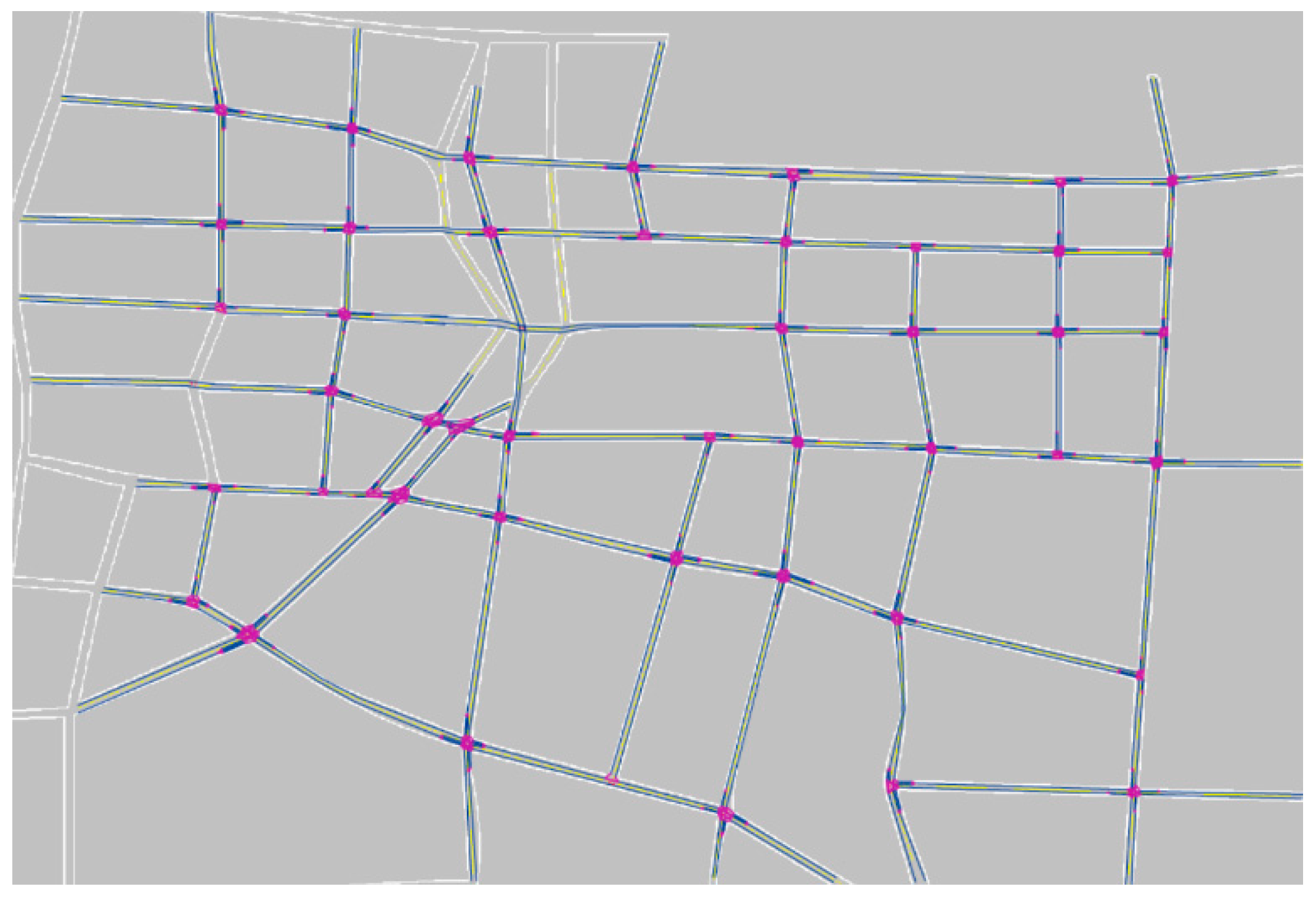
Based on the obtained basic data, the traffic conditions in the road network were simulated using Vissim 6.0 software. The actual conditions of the roads were surveyed prior to conducting simulations, and various types of road information (e.g., number of lanes, length of incoming roads, special lanes, and special traffic control) were recorded in detail. Based on this information, the road network was simulated as shown in Figure 3.

Some road junctions were not represented in the simulated road network. Most of these unrepresented road junctions were connected to the simulated road network by interchanges (underpass tunnels). A few of these unrepresented road junctions were connected to the simulated road network by ramps. Because no electronic traffic monitoring points are set up at these road junctions, the traffic flow through these road junctions was estimated and included in our simulations.

For intersections with no electric traffic monitoring points, the estimation of traffic flow needed to refer to the monitoring point data of the adjacent intersections. In the data detected at the upstream monitoring points, the information for a vehicle heading to the intersection without monitoring points was extracted. After that, the vehicle was retrieved in the data of other downstream monitoring points to find the location where the vehicle location was next collected. The two collected locations were used as the start and end points of the vehicle path, and the shortest path model was used to calculate the possible trajectory of the vehicle in the area without detection equipment by combining the travel times of the road sections. The path with the highest selection probability was identified as the vehicle path. Finally, all paths were counted, and the results were used as the number of vehicles without monitoring points.

3.4. Calibration of the Road Network

Because the investigated road network contains many intersections, calibrating traffic simulation data using a single metric could lead to large errors. In our experiments, calibration using two indicators reduced the error by about 5% to 12% compared to a single indicator. Therefore, data calibration was performed from two perspectives, namely vehicle speed on individual road sections and traffic flow through individual intersections.

In the traffic volume calibration, the data extracted via the license plate recognition system were first counted according to the intersections, and we could obtain the data regarding the number of vehicles passing an individual intersection in a real environment. Then, a data collector was placed in front of the intersection stop line of the simulated road network. The number of vehicles passing in that direction could be obtained with this collector. The count results from each direction of the intersection were summed to obtain the number of vehicles passing an individual intersection in the simulation environment. The error rate was calculated by comparing it with the results of the real count.

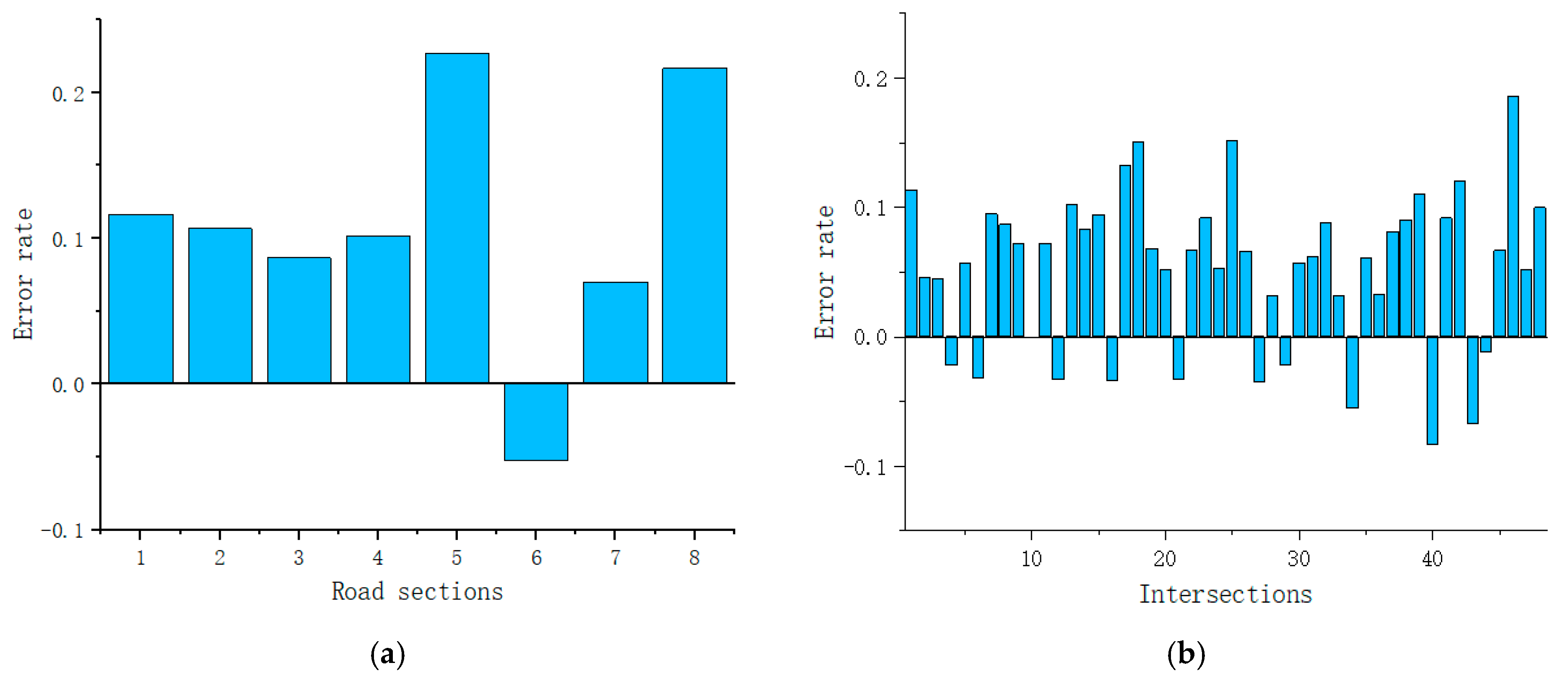
When the travel time calibration was performed, the vehicles that were detected at the two adjacent intersections of a given road segment in the real data were first screened. The difference in detection time was used as the travel time of that road segment. The average value was calculated as the travel time in the real environment after excluding the abnormal data. And then, in the simulated road network, the start and end points of the travel time detectors were set at the two intersections, and the simulated travel time of the road section was measured. It was compared with the real calculated value to derive the error rate. The specific results are shown in Figure 4.

Travel times on eight road sections in the road network were calibrated. The results reveal that in general, the simulated travel time was longer than the actual travel time, potentially because the simulated lane change time was longer than the actual lane change time. However, the simulated travel time on road section #6 was shorter than the actual travel time as a result of low traffic density during the simulated time period. The error rate was negative, and the traffic flowed smoothly.

The traffic flow (vehicles/h) through individual intersections was calibrated by comparing the simulated and observed (traffic data from license plate recognition systems) traffic flows. The maximum error rate was 18% (intersection #46), and the mean error rate was 5.4%.

After calibration, the simulated road network maintained a low error rate with the parameters in the real road network. This allows the simulated road network to approximate the real road environment. The experimental results obtained in the simulated road network can better predict the actual application results.

However, the real road environment contains many factors, and the road state is time-varying. The simulated road network cannot fully include these elements and has certain limitations. Nonetheless, in the case of unknown experimental effects, using a simulated road network for simulation testing is still a good way to save time and money.

4. Network-Partitioning-Based Distributed Traffic Control

4.1. Normalization Algorithm

The level of congestion on individual road sections was rated according to the traffic speed and traffic congestion zoning method provided in the GA/T 115-2020 Evaluation Method for Road Traffic Congestion Levels [54], as shown in

Table 2. Mean-traffic-speed-based rating of the level of congestion of urban arterial roads and secondary arterial roads.

Speed Limit	Mean Traffic Speed
80	≥45	[30, 45)	[20, 30)	[0, 20)
70	≥40	[30, 40)	[20, 30)	[0, 20)
60	≥35	[30, 35)	[20, 30)	[0, 20)
50	≥30	[25, 30)	[15, 25)	[0, 15)
40	≥25	[20, 25)	[15, 20)	[0, 15)
<40	[25, speed limit)	[20, 25)	[10, 20)	[0, 15)
Level of traffic congestion	Smooth	Light congestion	Moderate congestion	Severe congestion
Color indicator
Rating of congestion	Level IV	Level III	Level II	Level I

Note: The level of congestion on branch roads was rated similarly.

.

In the following equation, v_u is the critical speed representing the transition between smooth traffic and light traffic congestion, v_ij is the average vehicle speed for the road section between between the ith and jth intersections, and v_d is the critical speed representing the transition between moderate and severe congestion. For designating the level of congestion on a road S_ij, when v_ij ≥ v_u, the traffic on the road is smooth, and S_ij is assigned a value of zero. When v_ij < v_d, the road is severely congested, and S_ij is assigned a value of one. When v_u > v_ij ≥ v_d, the level of congestion on the road is calculated based on the two critical speeds and actual traffic speed, and the value of S_ij falls between zero and one.

$$S_{ij}=\left\{\begin{array}{cc}0& v_{ij}⩾v_u\\ \frac{v_u-v_{ij}}{v_u-v_d}& v_u>v_{ij}⩾v_d\\ 1& v_{ij}<v_d\end{array}\right.$$

(1)

The level of congestion on an incoming road is calculated based on the traffic flow, number of lanes, and traffic capacity of individual lanes. The level of congestion at the ith intersection in the jth incoming direction is denoted as RF_ij, which is calculated as

$$R{F}_{ij}=\frac{q_{ij}}{c\times n_{ij}}$$

(2)

The effects of the upstream and downstream road sections and intersections on a specific road are considered. The level of congestion at the ith intersection is denoted as N_i and calculated as

$$N_i=\frac{\underset{j}{max}\hspace{0.17em}\left(R{F}_{ij}\right)+\underset{j}{max}\hspace{0.17em}\left(S_{\mathrm{i}\mathrm{j}}\right)}{2}$$

(3)

The dynamic state of congestion on roads is analyzed using this metric. The static state of congestion is analyzed by considering the distance between pairs of adjacent intersections as

$$FS(i,j)=\left\{\begin{array}{cc}1& a(i,j)=1,l_{i,j}⩽200\\ {\mathrm{e}}^{-\frac{l_{i,j}-200}{{\sigma }_X}}& a(i,j)=1,l_{i,j}>200\\ 0& a(i,j)=0\end{array}\right.$$

(4)

where a(i,j) is the state of connection between the ith and jth intersections, which is assigned a value of one if the two intersections are directly connected and is assigned a value of zero otherwise. Previous studies have shown that a pair of intersections within 200 m of each other are strongly associated [28]. Therefore, if a pair of intersections are connected and separated by a distance of less than 200 m, FS is assigned a value of one. Here, σ_x is a correction coefficient.

For a pair of intersections separated by a distance greater than 200 m, the value of FS decreases as the distance increases. This distance assumption currently applies only to urban roads in China. The distance threshold for strong correlation may vary from country to country due to many differences in driving habits, construction standards, etc.

The association between a pair of intersections φ_ij is obtained based on the dynamic metric N and static metric FS as

$${\phi }_{ij}=FS(i,j)\times \mathrm{e}\mathrm{x}\mathrm{p}\left[-{\left(\frac{\left|N_i-N_j\right|}{{\sigma }_y}\right)}^2\right]$$

(5)

This equation indicates that the association between a pair of connected intersections φ_ij decreases as the difference between the levels of congestion at the two intersections N_i increases. Therefore, intersections with similar traffic conditions are more likely to be clustered in the same subnetwork.

4.2. Preliminary Partitioning of a Road Network

During the preliminary partitioning of a road network, it is abstracted as a graph G consisting of intersections and the roads connecting them. First, the graph G is partitioned into two parts A and B, where $A\cup B=G$ and $A\bigcap B=\mathrm{\varnothing }$, meaning all edges between A and B are removed. The sum of the weights of the removed edges is defined as

$$cut\left(A,B\right)={\sum }_{u\in A,v\in B}\omega \left(u,v\right),$$

(6)

where ω(u,v) is the weight of the edge connecting nodes u and v. When the value of $cut\left(A,B\right)$ is smallest, it represents the optimal result for the partition of A and B. Repeating this process can continuously dichotomize the graph. However, it may partition some isolated points into a separate subgraph, which is meaningless. To avoid generating such an independent partitioning, the normalized cut (Ncut) is used to measure the similarity of subgraph A and subgraph B, which is calculated as follows:

$$Ncut\left(A,B\right)=\frac{cut\left(A,B\right)}{assoc\left(A,G\right)}+\frac{cut\left(A,B\right)}{assoc\left(B,G\right)},$$

(7)

where assoc(A,G) is the association between subgraph A and graph G. If there is an isolated point that becomes a separate subgraph A, then the value of assoc(A,G) will be small. In general, the smaller the value of Ncut in Formula (7), the better the result of partitioning subgraph A and subgraph B.

Ensuring a low similarity between subgraphs is one of the requirements for graph partitioning. Furthermore, the nodes inside the subgraphs should have high similarity, which indicates that they are effectively partitioned into the same class. Therefore, the normalized association (Nassoc) is used to characterize the similarity within the subgraphs, which is calculated as follows:

$$Nassoc\left(A,B\right)=\frac{assoc\left(A,A\right)}{assoc\left(A,G\right)}+\frac{assoc\left(B,B\right)}{assoc\left(B,G\right)},$$

(8)

and assoc(A,A) is the association within subgraph A. A higher value of $Nassoc\left(A,B\right)$ means a higher degree of similarity within the subgraph. In summary, the objective of normalized partitioning is to minimize the Ncut between subgraphs while maximizing the Nassoc within subgraphs. Here, assoc(A,V) is equal to the sum of assoc(A,A) and cut(A,B). Therefore, the relationship between the two measures Ncut and Nassoc can be described as

$$Ncut\left(A,B\right)=2-Nassoc\left(A,B\right).$$

(9)

The minimum value of Ncut can be derived using the following characteristic equation:

$$\left(D-W\right)x=\lambda Dx,$$

(10)

where W is the edge weight matrix of graph G, and D is the degree matrix of W. Therefore, the steps for preliminarily partitioning a road network using the normalization algorithm can be summarized as follows:

(1)

The road network is abstracted as a graph G with intersections represented as the nodes, road sections represented as edges, and the associations between nodes represented as the weights of edges. Therefore, an edge weight matrix W can be obtained.

(2)

The characteristic equation is solved.

(3)

Graph G is partitioned according to the eigenvectors corresponding to the obtained eigenvalues.

(4)

If the number of nodes in a graph is greater than 20, then the above steps are repeated until the number of nodes in the graph is less than or equal to 20.

4.3. Control of Traffic Interflow at Subnetwork Boundaries

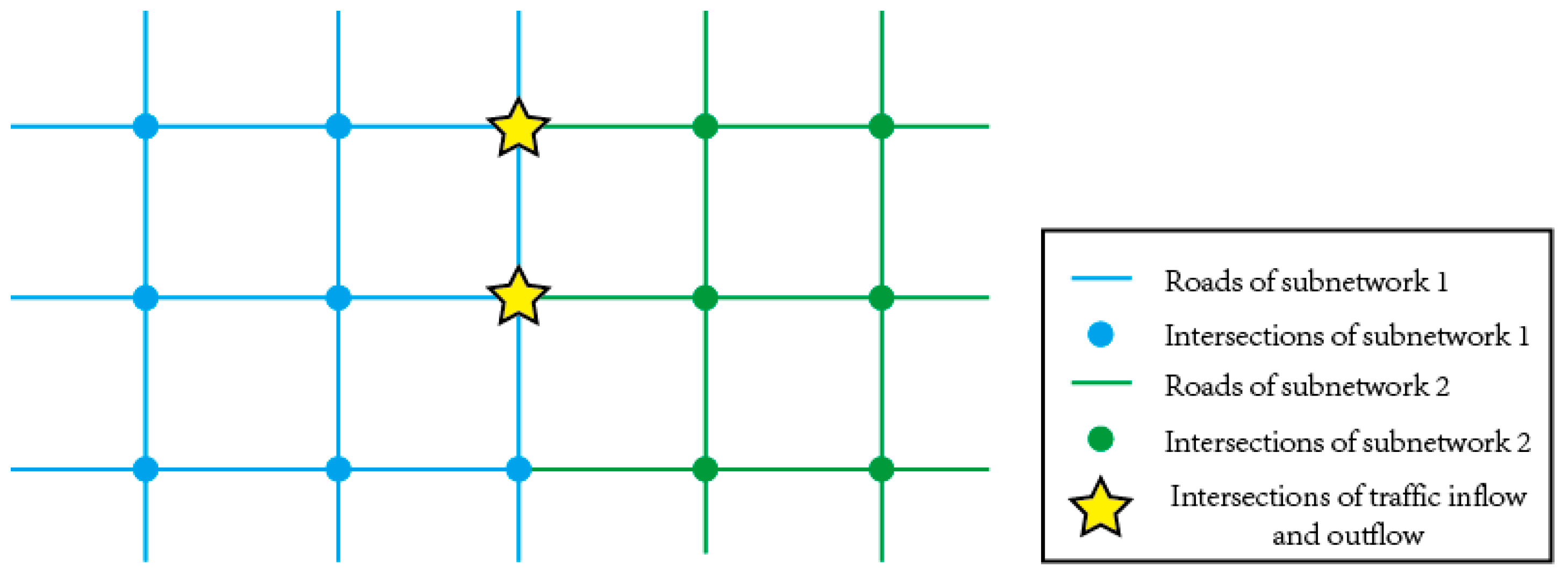
Once network partitioning is completed, the traffic interflows between the resulting subnetworks must be controlled to ensure that the traffic pressure in each subnetwork remains at an acceptable level. Therefore, the traffic interflow that points at subnetwork boundaries must be defined.

After an intersection is selected to serve as a point of traffic interflow between a pair of adjacent subnetworks, the traffic pressure on the corresponding roads increases. When the traffic interflow is low, the traffic pressure can be partially alleviated by adjusting the signal time. When the traffic interflow is large, it is possible that the desired traffic interflow cannot be achieved in a single optimization cycle. Additionally, the desired traffic interflow may exceed the traffic capacity of the intersection, leading to more severe congestion. By referencing previous studies, two intersections were configured at each subnetwork boundary for traffic inflow and outflow to relieve traffic pressure and increase traffic interflow capacity at boundaries, as shown in Figure 5.

For a subnetwork, its traffic state can be roughly divided into three states: unsaturated state, saturated state, and oversaturated state. If the real-time traffic volume of a subnetwork can be in the saturated state, the road resources can be fully utilized, and no serious congestion will occur. To achieve this effect, the threshold for traffic flow within individual subnetworks is defined using a series of parameters.

The critical values of the unsaturated, saturated, and oversaturated stages are denoted as B and C. Based on the macroscopic fundamental diagram of the road network, the values of B and C corresponding to the different subnetworks can be calculated [55]. When the traffic flow is less than B, the traffic in the subnetwork flows smoothly. When the traffic flow is greater than C, the traffic in the subnetwork is severely congested. Assuming that the number of real-time vehicles in the subnetwork at the end of the k control cycle is A, its value is influenced by the vehicle count a at the end of the k − 1 cycle and the vehicle counts b and c of the inflow and outflow of the k − 1 cycle. The relationship is shown in the following formula:

$$A=a+b-c,$$

(11)

At the end of each control cycle, the real-time traffic volume in the subnetwork can be calculated using Formula (11). Then its value is compared with (B, C). If it is not within this range, the state shift probability matrix must be updated. And the signal timing of the traffic interflow intersection is adjusted to change the inflow and outflow volumes in the next cycle to ensure a stable traffic interflow. For example, if A > C, it means that the subnetwork is currently congested and in the oversaturation stage. It is necessary to reduce the inflow volume of vehicles and increase the outflow volume of vehicles in the next control cycle to make the traffic state of the subnetwork change from the oversaturation stage to the saturation stage.

It should be noted that at the end of each control cycle, it is necessary to compare whether the value of A is within the range of (B, C).

5. Results and Analysis

5.1. Partitioning Results

The study by Yin et al. [56] revealed that connectivity between subnetworks does not fail as the number of subnetworks k increases. Instead, the resulting subnetworks take on more diversified traffic characteristics. To ensure the effectiveness of traffic control at subnetwork boundaries, partitioned subnetworks should not be excessively small. The investigated road network was partitioned into different numbers (three, four, and five) of subnetworks to analyze the effects of different partitions. Figure 6 presents the results.

When the road network was partitioned into three subnetworks using the normalization algorithm, the boundaries between the resulting subnetworks were mostly arterial roads. Figure 7 and Figure 8 show the results of the partition using the GN algorithm and the experience-based manual method, respectively. From the results, the three partitioning methods are generally similar. Each subnetwork had an adequate number of intersections for within-subnetwork traffic control, regardless of whether the road network was partitioned into three, four, or five subnetworks.

5.2. Traffic Pressure

After network partitioning was completed, the traffic pressure in the road network was analyzed according to the ratings of traffic congestion defined in Table 1. Figure 9 presents the results.

The green color in Figure 9 represents low saturation (meaning low road utilization). Yellow represents medium saturation (meaning normal traffic conditions). Orange represents relatively high saturation (meaning that the road is fully utilized). Red represents oversaturation (meaning severe congestion). It can be seen that in the original condition, the distribution of traffic pressure on road sections is quite uneven.

Table 3. Results via statistics regarding the traffic pressure based on normalized algorithm.

Partitioning Situation	Number of Road Sections
	Green	Yellow	Orange	Red
Original condition	8	30	34	22
Partitioned into three subnetworks	6	23	54	11
Partitioned into four subnetworks	6	20	60	8
Partitioned into five subnetworks	6	24	52	12

shows the change of traffic pressure on road sections.

From Figure 9 and Table 3, it can be seen that the number of yellow road sections and red road sections decreased after partitioning and boundary control. And the number of orange road segments increased. This indicates that after zoning and boundary control, the traffic pressure on the road network was dispersed. This result indicates that distributed traffic control based on network partitioning using the normalization algorithm improves traffic conditions by alleviating traffic congestion on highly saturated roads by redirecting traffic to less saturated roads.

Regarding the degree of improvement, partitioning the road network into four subnetworks led to a more even congestion distribution. This indicates that under the premise of ensuring an adequate number of intersections in each subnetwork, distributed traffic control via partitioning of the investigated road network into four subnetworks has the best effect in terms of improving traffic congestion. Figure 10 and Figure 11 show the control effect after the area division based on the GN algorithm and experience-based manual method, respectively.

Table 4. Results via statistics regarding the traffic pressure based on GN algorithm.

Partitioning Situation	Number of Road Sections
	Green	Yellow	Orange	Red
Original condition	8	30	34	22
Partitioned into three subnetworks	6	23	54	11
Partitioned into four subnetworks	6	20	60	8
Partitioned into five subnetworks	6	24	52	12

and

Table 5. Results via statistics regarding the traffic pressure based on experience-based manual method.

Partitioning Situation	Number of Road Sections
	Green	Yellow	Orange	Red
Original condition	8	30	34	22
Partitioned into three subnetworks	6	23	54	11
Partitioned into four subnetworks	6	20	60	8
Partitioned into five subnetworks	6	24	52	12

show the change of traffic pressure on road sections after subnetwork partitioning using the GN algorithm and experience-based manual method.

Comparing Table 3, Table 4 and Table 5, it can be seen that after subnetwork partitioning and boundary control, the average effect of all three methods on road network pressure is better than the original condition. The number of red road sections in Table 5 is much higher than in Table 3 and Table 4. Although the experience-based manual method also makes the road network have more orange road sections, the excessive number of red road sections indicates that the method is not effective in balancing the pressure on the road network. It means that the empirically based manual method is not as effective at controlling as the other two methods. This also indicates that data-based partitioning is more helpful in improving the control effectiveness of the road network. The comparison of the normalized algorithm and the GN algorithm for each category of partitioning results shows that although both algorithms reduce the pressure on congested road sections, there are still some differences in some sections, indicating that different partitioning methods have some influence on the effect of regional coordination control.

5.3. Analysis of Local Traffic Pressure

The road sections in the investigated road network differed significantly in terms of road classification, lane width, and traffic flow. The investigation results reveal that the arterial roads in the investigated road network had more congested sections. Therefore, the traffic speed variations on two arterial roads (i.e., at intersections #44, 9, 10, 11, 12, and 31 and intersections #16, 17, 18, 19, and 33, respectively, covering a total of 13 road sections) were analyzed using three different methods (normalization algorithm, GN algorithm, and an experience-based manual method) separately. Figure 12 presents the results.

The results show that vehicle speeds improved on all road segments after optimization, regardless of whether the area was classified using the normalization algorithm or the GN algorithm. It is noteworthy that the vehicle speed on road segment 7 was higher than the other road segments before optimization. Road segment 7 is located at the boundary of the study area and is far from any heavily congested road segments. This allows this road to have high traffic speeds prior to optimization. Optimization can reduce traffic pressure on congested road segments and increase vehicle speeds. Therefore, the vehicle speed of segment 7 also increased after optimization. However, the other road sections have more vehicles and are more congested, so the optimized vehicle speed increased even more.

Table 6. Comparisons of improvements in local traffic speed achieved by different methods.

Partitioning Method	Traffic Speed Improvement (%)
	Three Subnetworks	Four Subnetworks	Five Subnetworks
Normalization algorithm	28.0%	39.0%	27.8%
GN algorithm	16.3%	27.8%	20.4%
Experience-based manual partition	14.0%	18.6%	18.3%

shows the improvement effect of different methods in Figure 12. The average speed of the 13 road segments in the original state was 19.42 km/h. The values in Table 4 indicate the percentage increase in the average speed of the 13 road segments compared to the original state after road network partitioning and boundary control.

One can see that for the normalization algorithm, partitioning the investigated road network into four subnetworks yielded the best improvement in traffic speed. For the GN algorithm, partitioning the road network into four subnetworks yielded better overall improvement than partitioning the road network into five subnetworks. However, for some road sections, partitioning the road network into five subnetworks yielded better improvement than partitioning the road network into four subnetworks. As shown in Figure 12 for the arterial roads, partitioning the road network into four subnetworks yielded the best improvement when using either the normalization or GN algorithm. Additionally, despite the manual partitioning method improving the traffic speed on local road sections in general, traffic control using metric-based partition algorithms yielded greater improvements.

6. Conclusions

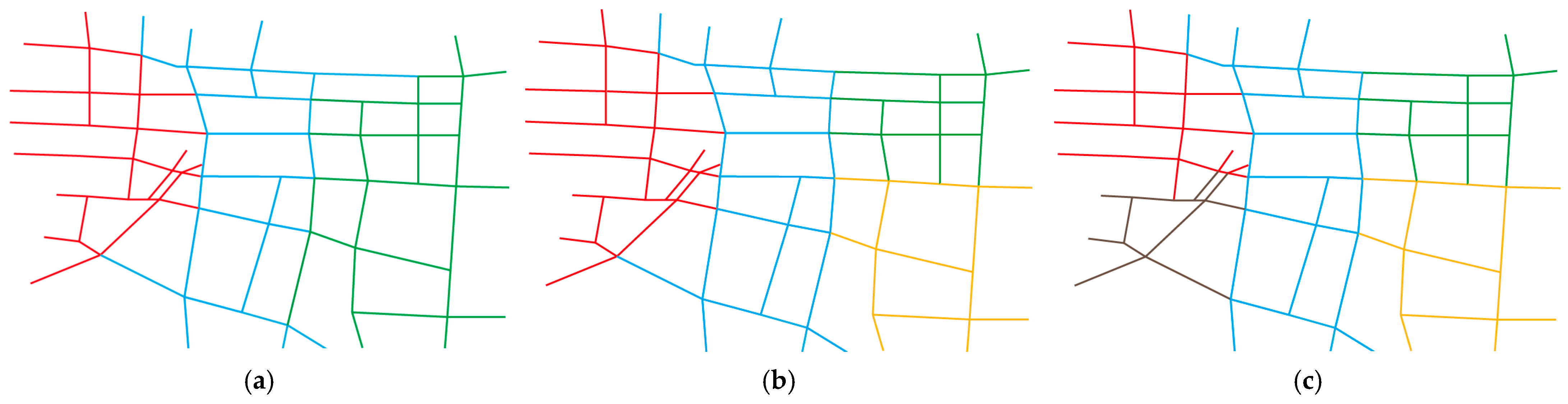
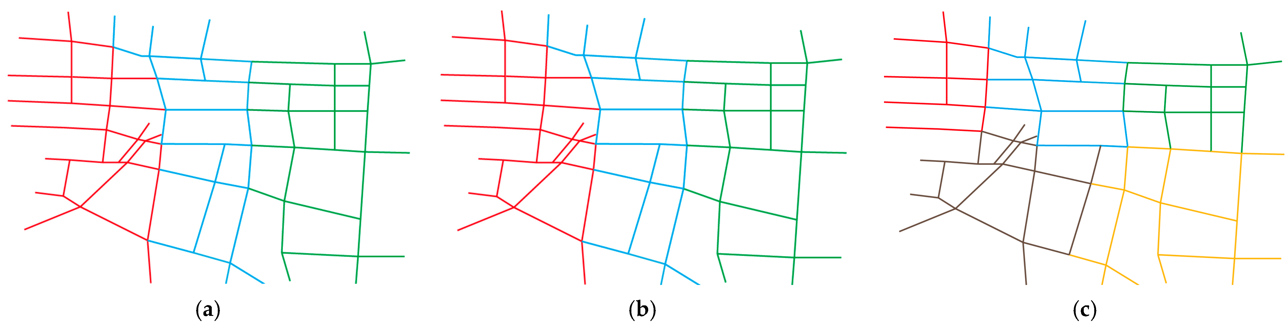
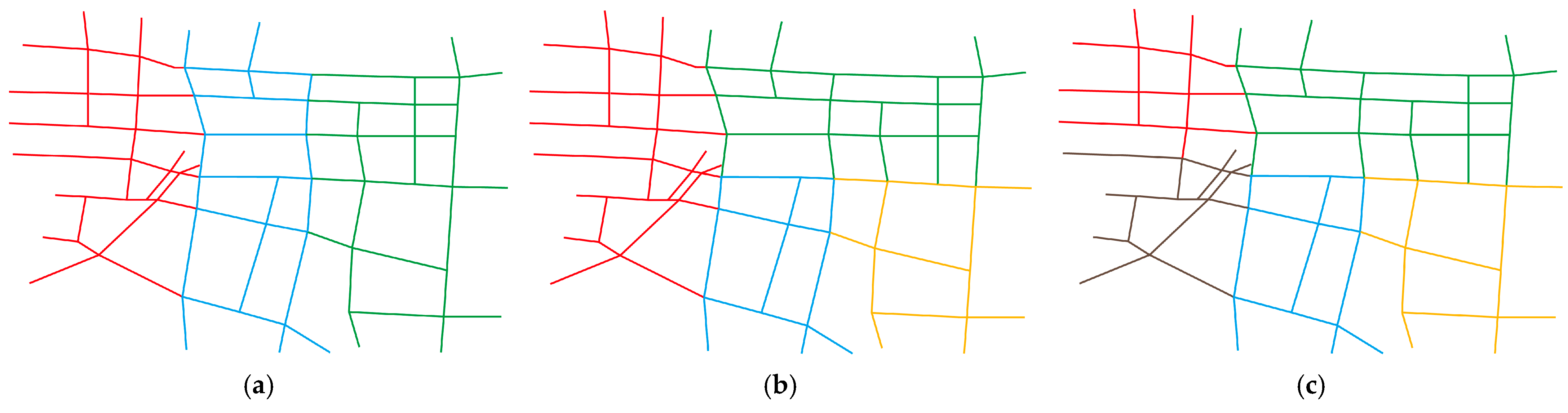
In this study, the traffic conditions in a real road network were investigated. First, the road network was simulated using the Vissim software, and the simulations were calibrated from multiple perspectives. Next, the road network was partitioned using the normalization algorithm. Two intersections were configured at the boundary between each pair of resulting subnetworks, and a maximum threshold was defined for traffic flow between each pair of subnetworks to balance between-subnetwork traffic pressure. Finally, the partitioning results yielded via the normalization algorithm were compared with those yielded via the GN algorithm and an experience-based manual method in terms of the improvement of both overall and local traffic pressure. The results can be summarized as follows:

(1)

For all road network partitioning methods, partitioning improved traffic congestion for partitioning into three, four, or five subnetworks. However, partitioning the road network into different numbers of subnetworks yielded different degrees of improvement.

(2)

Road-network-partitioning-based distributed traffic control improved the traffic pressure when using either the normalization or GN algorithm. However, different partitioning methods had different effects on the traffic control at subnetwork boundaries, meaning they improved traffic pressure to varying degrees.

(3)

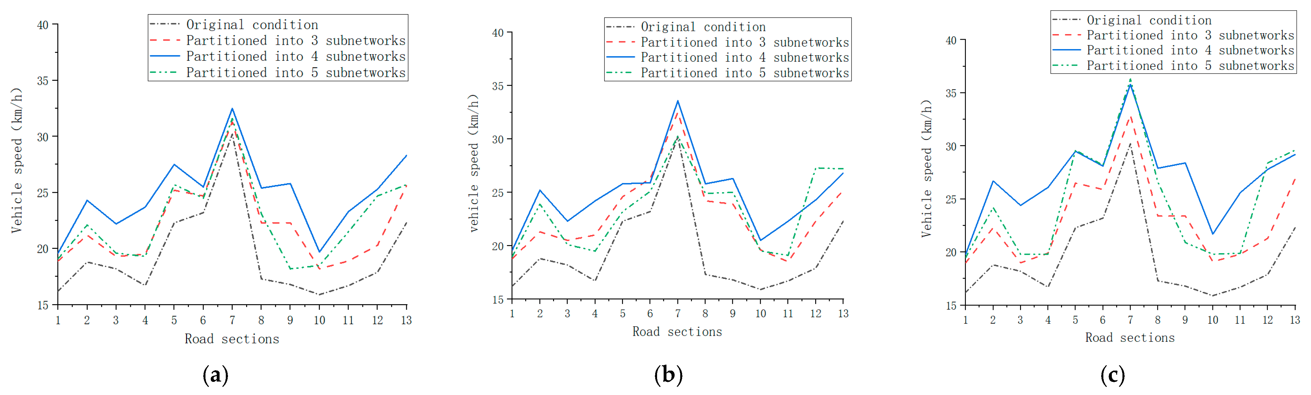
Road-network-partitioning-based traffic control improved the traffic speed when using either the normalization or GN algorithm. Partitioning the road network into four subnetworks yielded the greatest degree of improvement. Additionally, algorithm-based road network partitioning yielded greater improvements in traffic speed than the manual method.

(4)

Road-network-partitioning-based distributed traffic control using the normalization algorithm performed best in terms of balancing traffic pressure and improving traffic speed in the road network.

In the calibration of the simulated road network, we compared the simulated road network with the real data to make the simulated road network closer to the real state. The use of a simulated road network calibrated with real data for validation is also a feature of this paper. Calibration with real data requires a more complex calibration process than a fully hypothetical simulation environment. The process is very difficult. It is because of such a calibration process that the method can predict to some extent the effects of real applications. The partitioning method proposed in this paper can achieve better control results for the simulated road network, which means that the application of this method in the real environment should have similar results. This method can predict the effects of real applications to some extent. However, it should be noted that the condition of the real road network is complex and variable, and there are influencing factors that are not considered in this study. Therefore, the actual application effects may be slightly lower than the simulation results.

It is worth noting that if the intersection pressure at the subnetwork boundaries is high, vehicles will gather at these intersections to enter other subnetworks. The intersection pressure will increase. To improve this situation, it is not a bad idea to use multiple intersections for traffic interflow control. However, this has great limitations and challenges in controlling the whole road network and balancing the subnetwork traffic pressures. To further investigate the effect of boundary control on improving road network congestion, there is a plan to set a threshold for boundary intersections. Under this condition, the intersections used for traffic interflow control will be irregular. Two or more intersections will be used to satisfy traffic demand.