
Can the MODIS Data Achieve the Downscaling of GOME-2 SIF? Validation of Data from China


Abstract
:1. Introduction
2. Study Area and Data
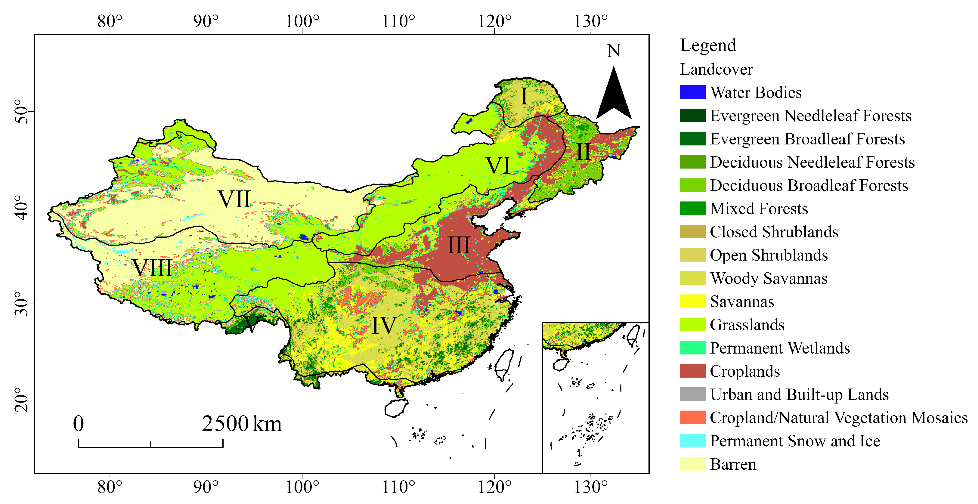
2.1. Overview of the Study Area
2.2. Data
3. Method
3.1. Downscaling Algorithm
3.2. Data Authenticity Test Method
4. Results and Analysis
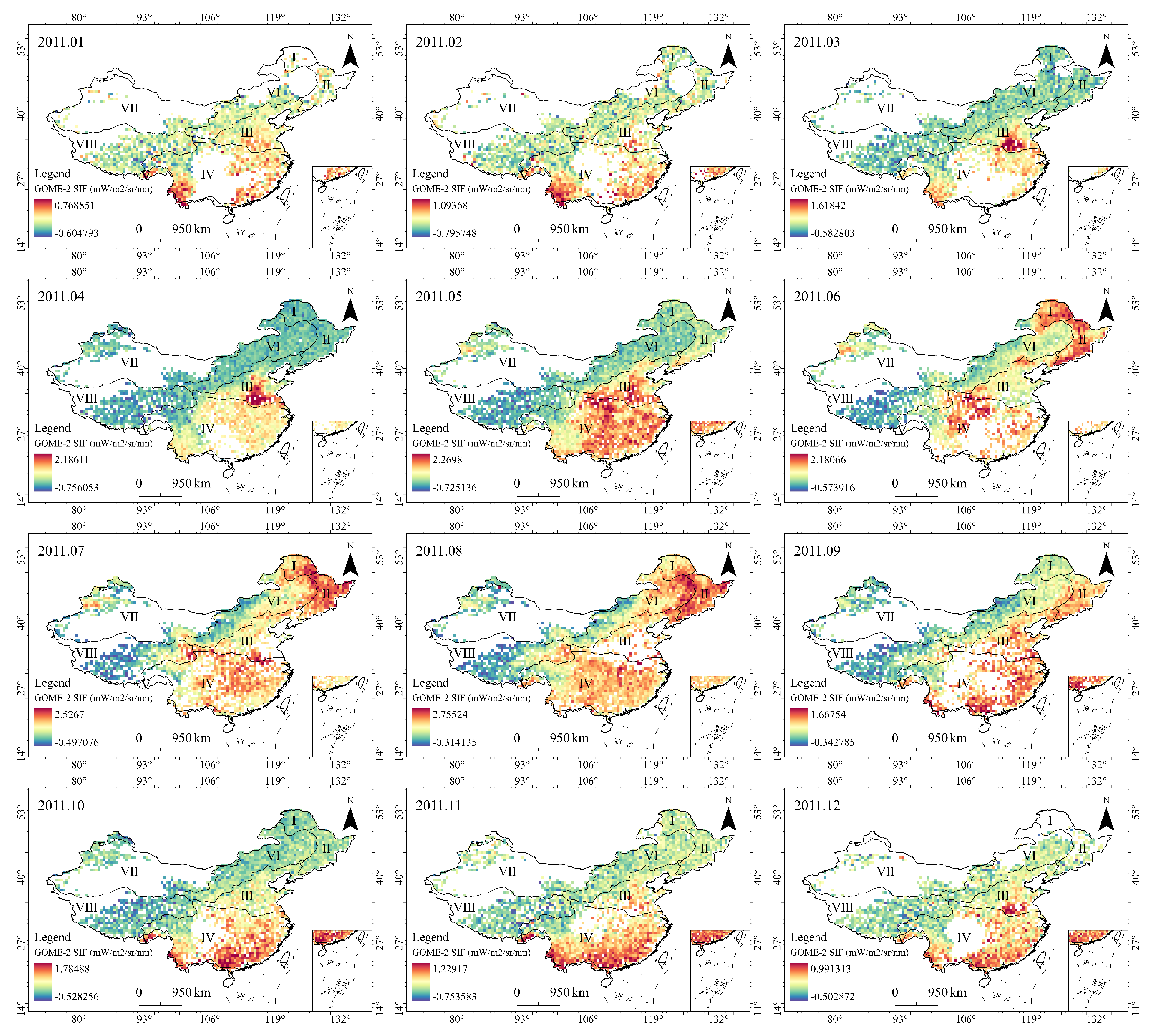
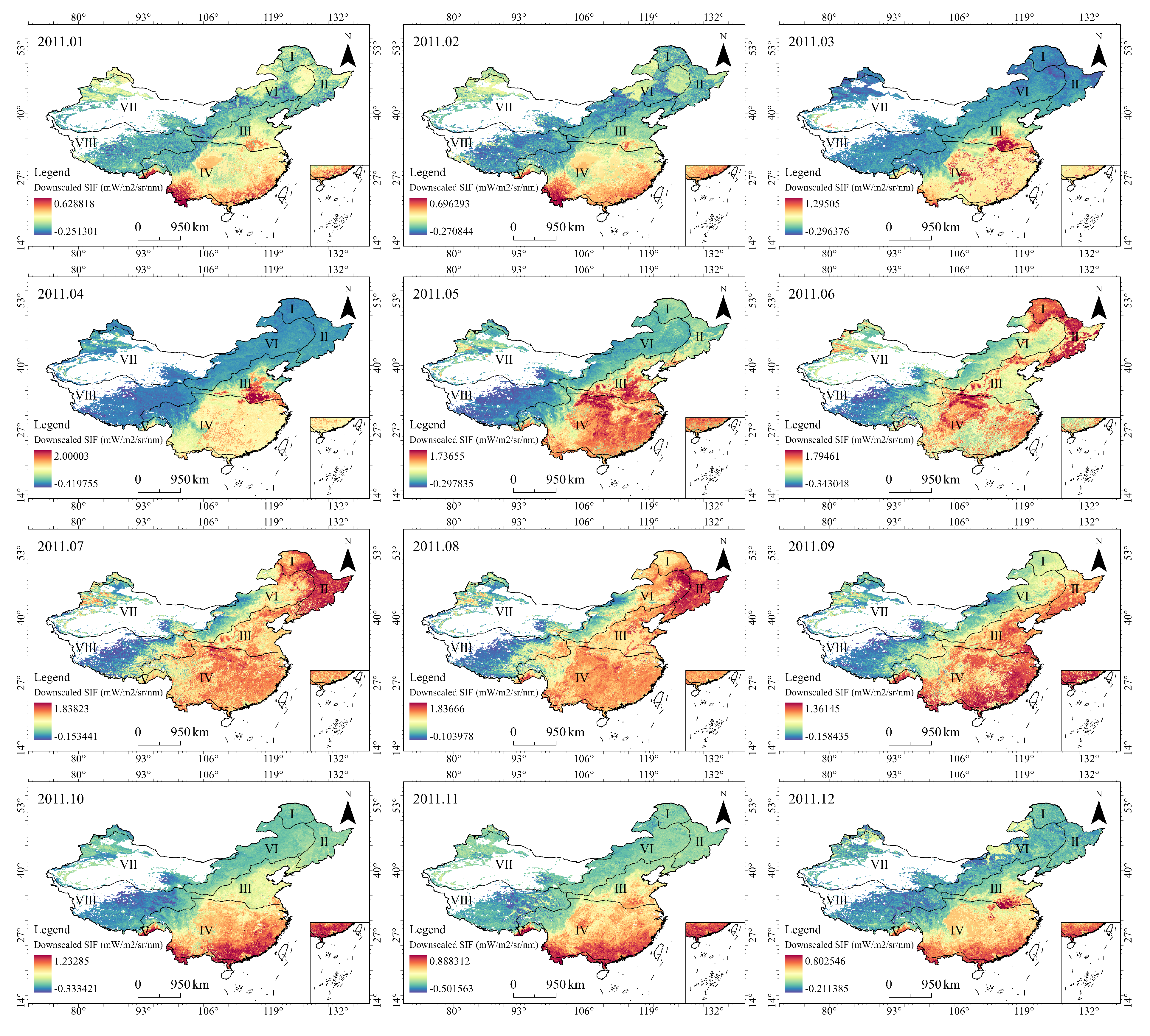
4.1. Downscale Results
4.2. Data Authenticity Check
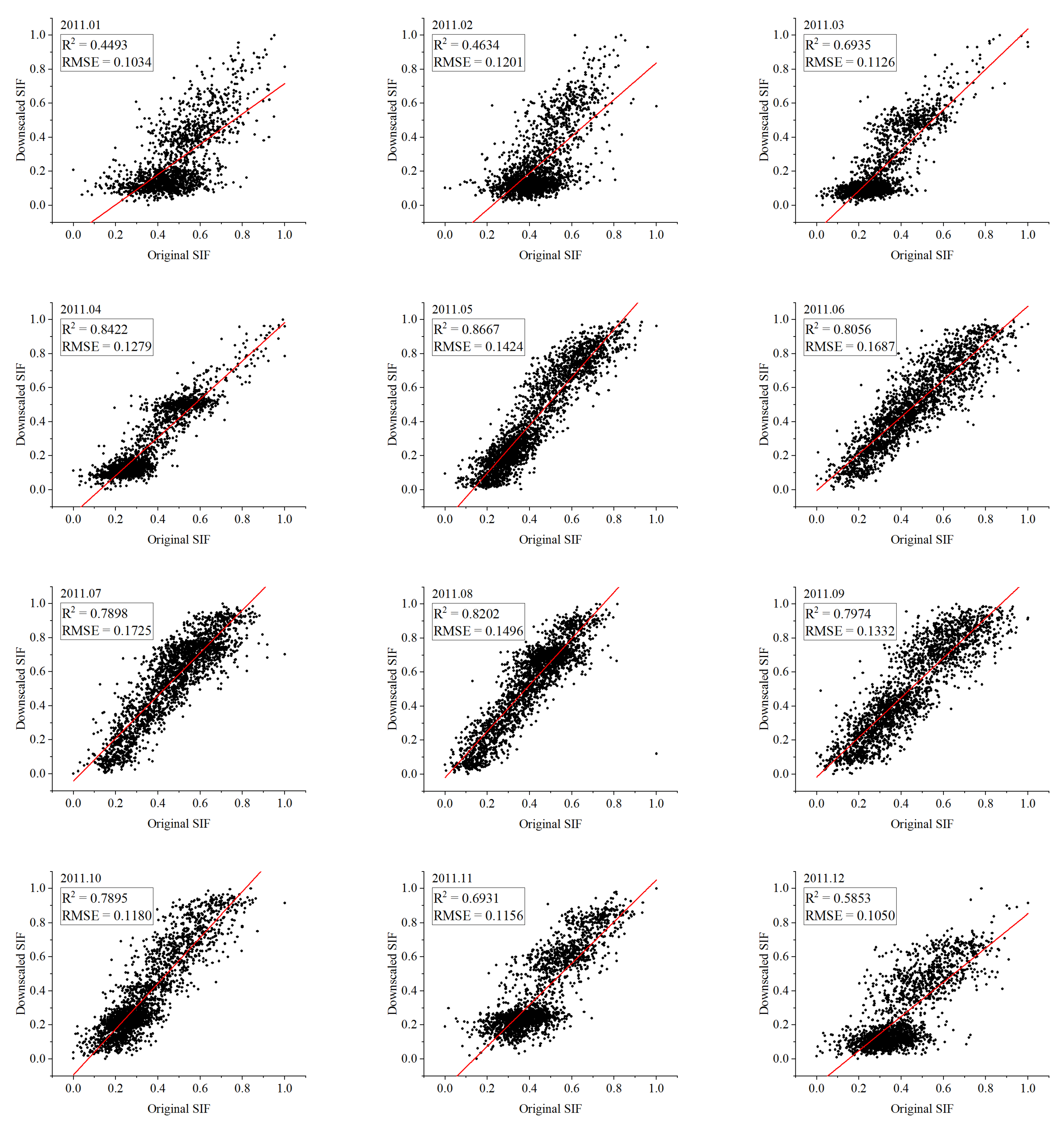
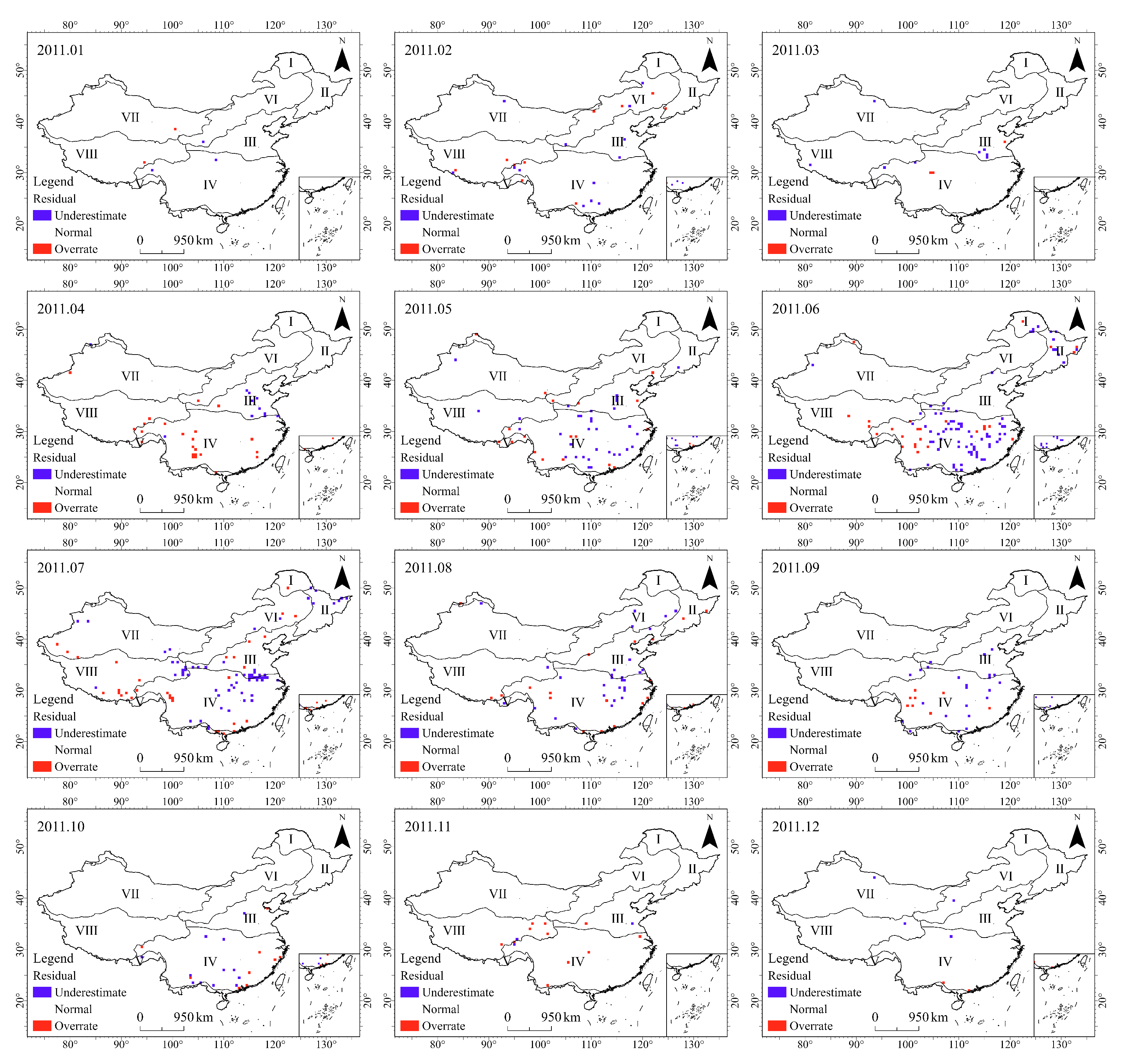
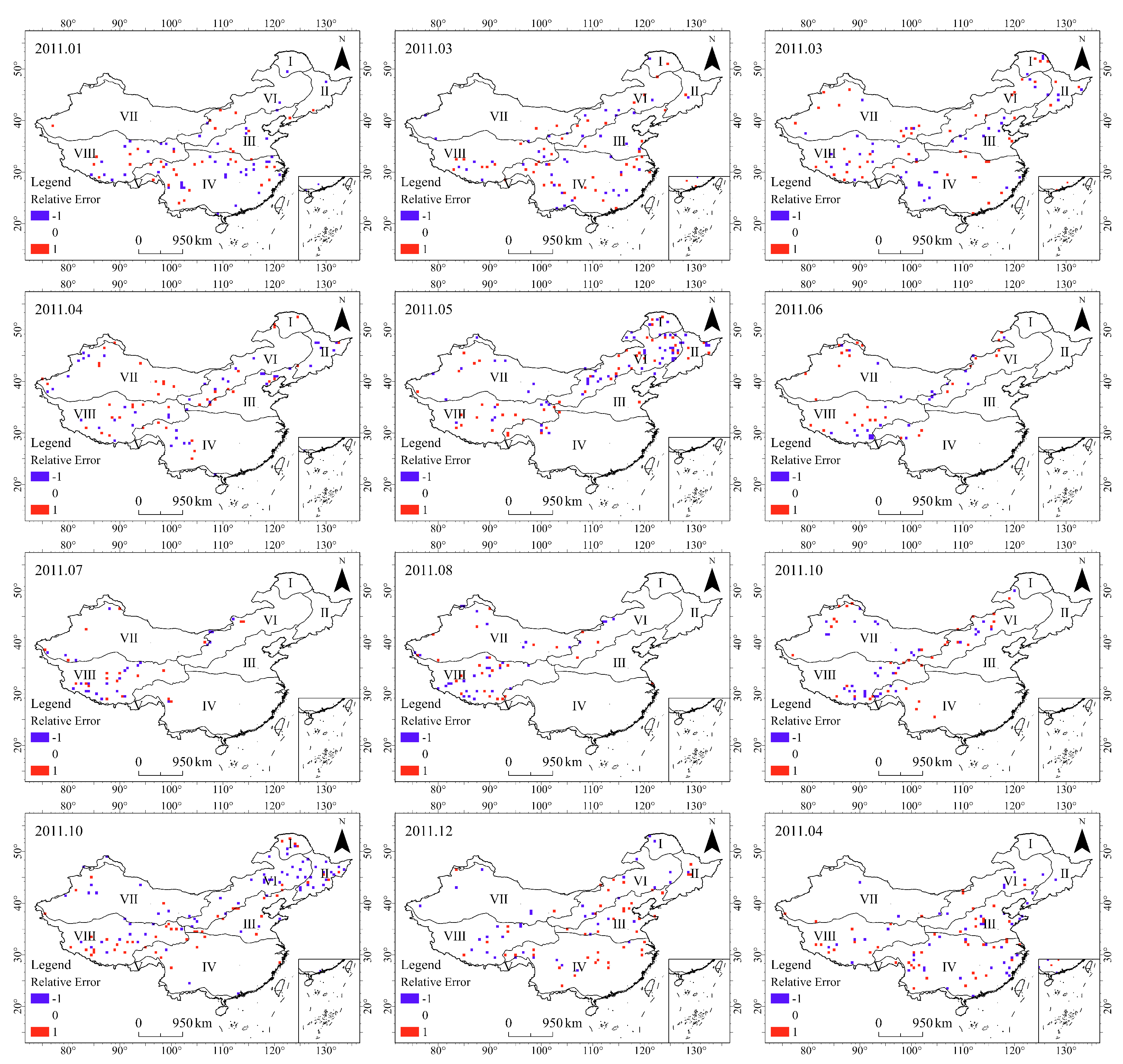
4.2.1. Monthly Scale Test
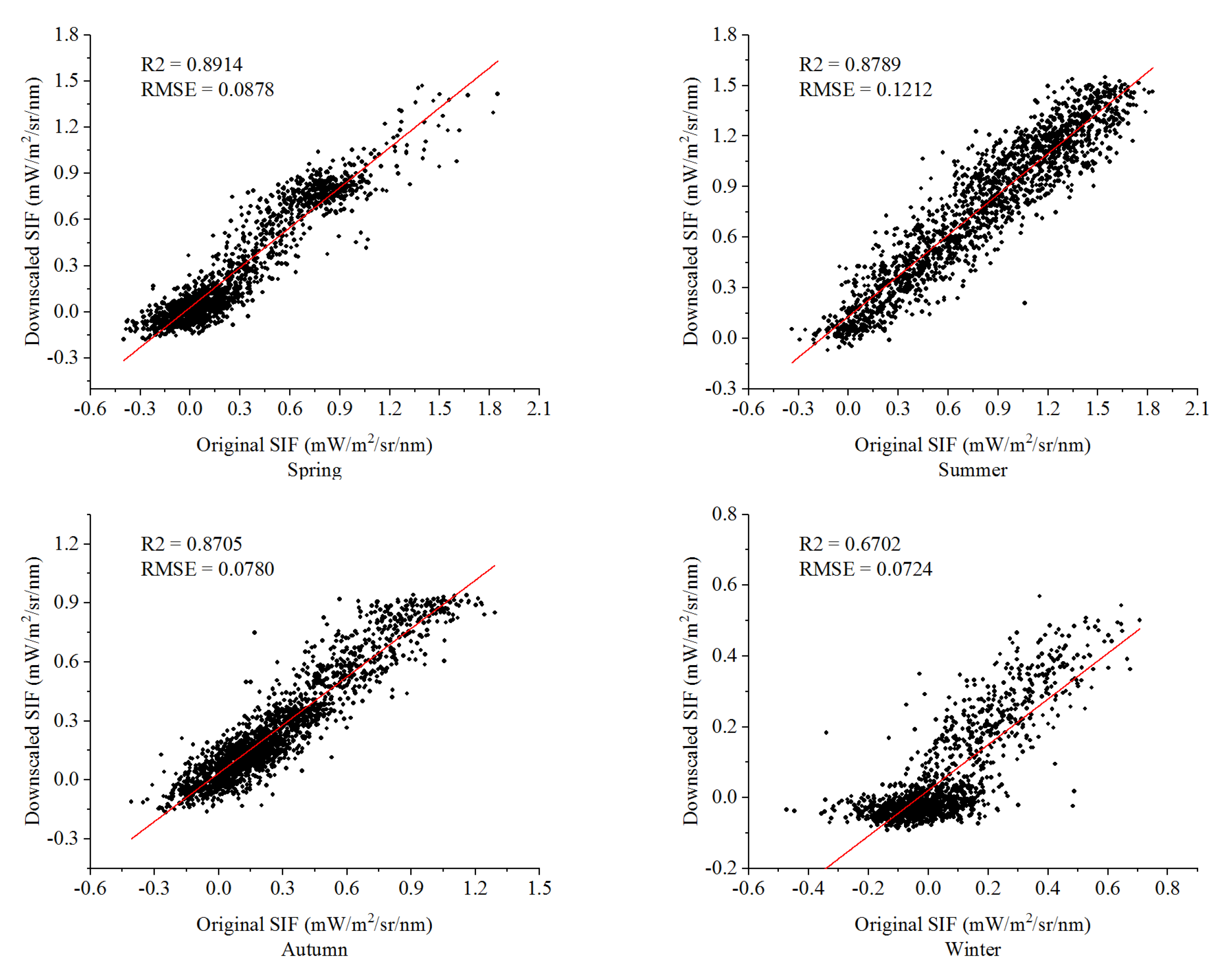
4.2.2. Seasonal Scale Test
4.3. Analysis of Factors Affecting the Accuracy of Downscaling Algorithms
4.3.1. SIF Data
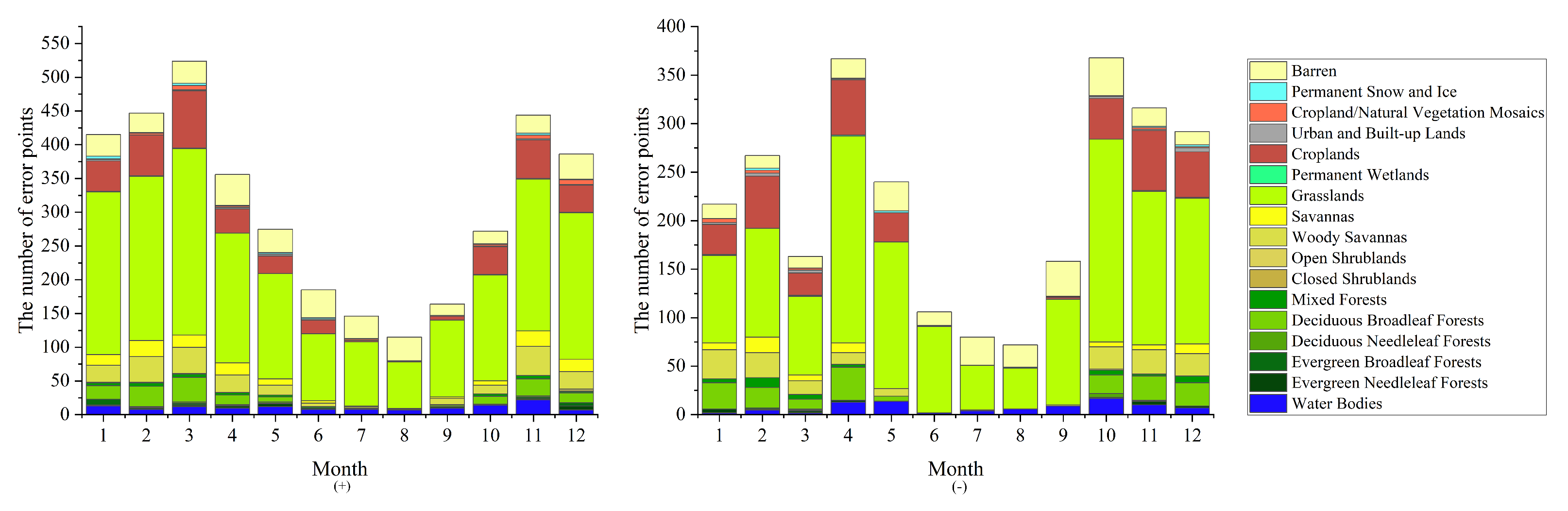
4.3.2. Land Cover Types
4.3.3. Climate Type
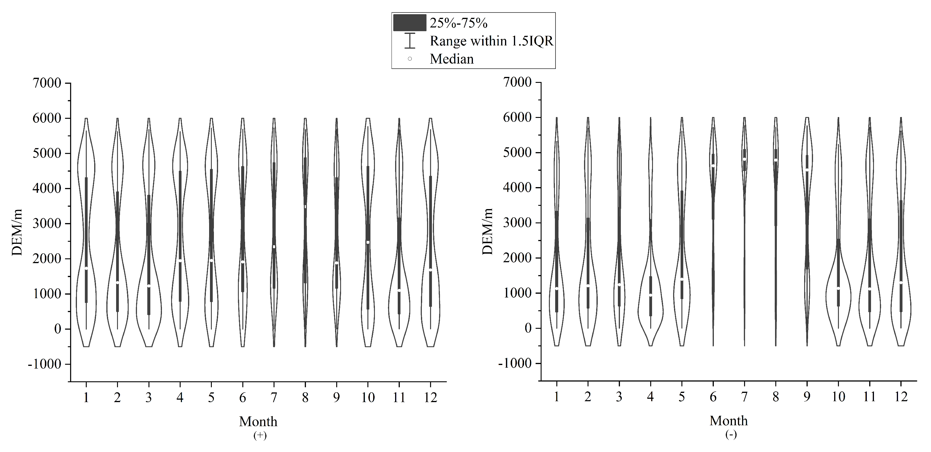
4.3.4. DEM
5. Conclusions
6. Discussion
Author Contributions
Funding
Institutional Review Board Statement
Informed Consent Statement
Data Availability Statement
Conflicts of Interest
References
- Porcar-Castell, A.; Tyystjärvi, E.; Atherton, J.; Van der Tol, C.; Flexas, J.; Pfündel, E.E.; Moreno, J.; Frankenberg, C.; Berry, J.A. Linking chlorophyll a fluorescence to photosynthesis for remote sensing applications: Mechanisms and challenges. J. Exp. Bot. 2014, 65, 4065–4095. [Google Scholar] [CrossRef] [PubMed] [Green Version]
- Mohammed, G.H.; Colombo, R.; Middleton, E.M.; Rascher, U.; van der Tol, C.; Nedbal, L.; Goulas, Y.; Pérez-Priego, O.; Damm, A.; Meroni, M.; et al. Remote sensing of solar-induced chlorophyll fluorescence (SIF) in vegetation: 50 Years of progress. Remote Sens. Environ. 2019, 231, 111177. [Google Scholar] [CrossRef] [PubMed]
- Gupana, R.S.; Odermatt, D.; Cesana, I.; Giardino, C.; Nedbal, L.; Damm, A. Remote sensing of sun-induced chlorophyll-a fluorescence in inland and coastal waters: Current state and future prospects. Remote Sens. Environ. 2021, 262, 112482. [Google Scholar] [CrossRef]
- Guanter, L.; Zhang, Y.; Jung, M.; Joiner, J.; Voigt, M.; Berry, J.A.; Frankenberg, C.; Huete, A.R.; Zarco-Tejada, P.; Lee, J.E.; et al. Global and time-resolved monitoring of crop photosynthesis with chlorophyll fluorescence. Proc. Natl. Acad. Sci. USA 2014, 111, E1327–E1333. [Google Scholar] [CrossRef] [PubMed] [Green Version]
- Sun, Y.; Frankenberg, C.; Wood, J.D.; Schimel, D.; Jung, M.; Guanter, L.; Drewry, D.; Verma, M.; Porcar-Castell, A.; Griffis, T.J.; et al. OCO-2 advances photosynthesis observation from space via solar-induced chlorophyll fluorescence. Science 2017, 358, eaam5747. [Google Scholar] [CrossRef] [Green Version]
- Joiner, J.; Yoshida, Y.; Vasilkov, A.; Yoshida, Y.; Corp, L.; Middleton, E. First observations of global and seasonal terrestrial chlorophyll fluorescence from space. Biogeosciences 2011, 8, 637–651. [Google Scholar] [CrossRef] [Green Version]
- Liu, X.; Liu, L. GOSAT satellite remote sensing retrieval of chlorophyll fluorescence. J. Remote Sens. 2013, 17, 1518–1532. [Google Scholar]
- Wen, J.; Köhler, P.; Duveiller, G.; Parazoo, N.; Magney, T.; Hooker, G.; Yu, L.; Chang, C.; Sun, Y. A framework for harmonizing multiple satellite instruments to generate a long-term global high spatial-resolution solar-induced chlorophyll fluorescence (SIF). Remote Sens. Environ. 2020, 239, 111644. [Google Scholar] [CrossRef]
- Joiner, J.; Guanter, L.; Lindstrot, R.; Voigt, M.; Vasilkov, A.; Middleton, E.; Huemmrich, K.; Yoshida, Y.; Frankenberg, C. Global monitoring of terrestrial chlorophyll fluorescence from moderate spectral resolution near-infrared satellite measurements: Methodology, simulations, and application to GOME-2. Atmos. Meas. Tech. Discuss. 2013, 6, 3883–3930. [Google Scholar] [CrossRef] [Green Version]
- Frankenberg, C.; O’Dell, C.; Berry, J.; Guanter, L.; Joiner, J.; Köhler, P.; Pollock, R.; Taylor, T.E. Prospects for chlorophyll fluorescence remote sensing from the Orbiting Carbon Observatory-2. Remote Sens. Environ. 2014, 147, 1–12. [Google Scholar] [CrossRef] [Green Version]
- Köhler, P.; Frankenberg, C.; Magney, T.S.; Guanter, L.; Joiner, J.; Landgraf, J. Global retrievals of solar-induced chlorophyll fluorescence with TROPOMI: First results and intersensor comparison to OCO-2. Geophys. Res. Lett. 2018, 45, 10–456. [Google Scholar] [CrossRef] [Green Version]
- Yu, L.; Wen, J.; Chang, C.; Frankenberg, C.; Sun, Y. High-resolution global contiguous SIF of OCO-2. Geophys. Res. Lett. 2019, 46, 1449–1458. [Google Scholar] [CrossRef]
- Duveiller, G.; Filipponi, F.; Walther, S.; Köhler, P.; Frankenberg, C.; Guanter, L.; Cescatti, A. A spatially downscaled sun-induced fluorescence global product for enhanced monitoring of vegetation productivity. Earth Syst. Sci. Data 2020, 12, 1101–1116. [Google Scholar] [CrossRef]
- Li, X.; Xiao, J. A global, 0.05-degree product of solar-induced chlorophyll fluorescence derived from OCO-2, MODIS, and reanalysis data. Remote Sens. 2019, 11, 517. [Google Scholar] [CrossRef] [Green Version]
- Hu, S.; Mo, X. Detecting regional GPP variations with statistically downscaled solar-induced chlorophyll fluorescence (SIF) based on GOME-2 and MODIS data. Int. J. Remote Sens. 2020, 41, 9206–9228. [Google Scholar] [CrossRef]
- Gentine, P.; Alemohammad, S. Reconstructed solar-induced fluorescence: A machine learning vegetation product based on MODIS surface reflectance to reproduce GOME-2 solar-induced fluorescence. Geophys. Res. Lett. 2018, 45, 3136–3146. [Google Scholar] [CrossRef]
- Ma, Y.; Liu, L.; Chen, R.; Du, S.; Liu, X. Generation of a global spatially continuous TanSat solar-induced chlorophyll fluorescence product by considering the impact of the solar radiation intensity. Remote Sens. 2020, 12, 2167. [Google Scholar] [CrossRef]
- Duveiller, G.; Cescatti, A. Spatially downscaling sun-induced chlorophyll fluorescence leads to an improved temporal correlation with gross primary productivity. Remote Sens. Environ. 2016, 182, 72–89. [Google Scholar] [CrossRef]
- Gómez-Ramírez, J.; Ávila-Villanueva, M.; Fernández-Blázquez, M.Á. Selecting the most important self-assessed features for predicting conversion to mild cognitive impairment with random forest and permutation-based methods. Sci. Rep. 2020, 10, 20630. [Google Scholar] [CrossRef]
- Justice, C.; Belward, A.; Morisette, J.; Lewis, P.; Privette, J.; Baret, F. Developments in the’validation’of satellite sensor products for the study of the land surface. Int. J. Remote Sens. 2000, 21, 3383–3390. [Google Scholar] [CrossRef]
- Shen, S.; Zhao, J.; Jia, J.; Zhao, Y. Comparison of different methods for downscaling TRMM precipitation data in Qilian Mountains. J. Mt. Sci. 2019, 37, 923–931. [Google Scholar]
- Yang, J.; Xiao, X.; Doughty, R.; Zhao, M.; Zhang, Y.; Köhler, P.; Wu, X.; Frankenberg, C.; Dong, J. TROPOMI SIF reveals large uncertainty in estimating the end of plant growing season from vegetation indices data in the Tibetan Plateau. Remote Sens. Environ. 2022, 280, 113209. [Google Scholar] [CrossRef]
- Cui, T.; Martz, L.; Zhao, L.; Guo, X. Investigating the impact of the temporal resolution of MODIS data on measured phenology in the prairie grasslands. GISci. Remote Sens. 2020, 57, 395–410. [Google Scholar] [CrossRef]
- Li, J.; Luo, J. Simulation of solar radiation in mountainous areas under clear sky. Geogr. Arid. Reg. 2015, 38, 120–127. [Google Scholar]
- Meroni, M.; Rossini, M.; Guanter, L.; Alonso, L.; Rascher, U.; Colombo, R.; Moreno, J. Remote sensing of solar-induced chlorophyll fluorescence: Review of methods and applications. Remote Sens. Environ. 2009, 113, 2037–2051. [Google Scholar] [CrossRef]
- Zhang, X.; Friedl, M.A.; Schaaf, C.B.; Strahler, A.H.; Hodges, J.C.; Gao, F.; Reed, B.C.; Huete, A. Monitoring vegetation phenology using MODIS. Remote Sens. Environ. 2003, 84, 471–475. [Google Scholar] [CrossRef]


| Month | R2 | RMSE | Bias |
|---|---|---|---|
| 1 | 0.4492 * | 0.1034 | −0.0425 |
| 2 | 0.4634 * | 0.1201 | 0.0896 |
| 3 | 0.6935 | 0.1126 | 0.0446 |
| 4 | 0.8422 | 0.1279 | 0.0273 |
| 5 | 0.8667 | 0.1424 | −0.0109 |
| 6 | 0.8056 | 0.1687 | −0.0215 |
| 7 | 0.7898 | 0.1725 | −0.0141 |
| 8 | 0.8202 | 0.1496 | −0.0048 |
| 9 | 0.7974 | 0.1332 | −0.0276 |
| 10 | 0.7895 | 0.1180 | −0.0292 |
| 11 | 0.6931 | 0.1156 | 0.0471 |
| 12 | 0.5853 | 0.1050 | 0.0215 |
| Residuals (mW/m2/sr/nm) | Type |
|---|---|
| <−0.5 | Underestimate |
| −0.5–0.5 | Normal |
| >0.5 | Overrate |
| Season | R2 | RMSE | Bias |
|---|---|---|---|
| Spring | 0.8914 | 0.0878 | −0.0161 |
| Summer | 0.8789 | 0.1212 | −0.0379 |
| Autumn | 0.8705 | 0.0780 | −0.0572 |
| Winter | 0.6702 | 0.0724 | 0.0194 |
| RE | Type |
|---|---|
| <−80% | −1 |
| others | 0 |
| >80% | 1 |
Disclaimer/Publisher’s Note: The statements, opinions and data contained in all publications are solely those of the individual author(s) and contributor(s) and not of MDPI and/or the editor(s). MDPI and/or the editor(s) disclaim responsibility for any injury to people or property resulting from any ideas, methods, instructions or products referred to in the content. |
© 2023 by the authors. Licensee MDPI, Basel, Switzerland. This article is an open access article distributed under the terms and conditions of the Creative Commons Attribution (CC BY) license (https://creativecommons.org/licenses/by/4.0/).
Share and Cite
Si, H.; Wang, R.; Wang, R.; He, Z. Can the MODIS Data Achieve the Downscaling of GOME-2 SIF? Validation of Data from China. Sustainability 2023, 15, 5920. https://doi.org/10.3390/su15075920
Si H, Wang R, Wang R, He Z. Can the MODIS Data Achieve the Downscaling of GOME-2 SIF? Validation of Data from China. Sustainability. 2023; 15(7):5920. https://doi.org/10.3390/su15075920
Chicago/Turabian StyleSi, Haixiang, Ruiyan Wang, Ruhao Wang, and Zixuan He. 2023. "Can the MODIS Data Achieve the Downscaling of GOME-2 SIF? Validation of Data from China" Sustainability 15, no. 7: 5920. https://doi.org/10.3390/su15075920