Pursuing the Sustainability of Real Estate Market: The Case of Chinese Land Resources Diversification

Abstract

Numerous studies have focused on the ripple effect in housing markets; however, these studies often fail to grasp the critical role of commercial real estate land use when forming a real estate portfolio. We argue that spreading an investment across various land-use assets—namely, diversification—may be effective in stabilizing and balancing China’s housing market through the introduction of the ripple effect. In six Chinese mega-cities, the cointegration system is initially used to prove the existence of ripple effects. A causality test can then identify the source cities: Beijing and Chongqing in the residential market, and Shenzhen and Chongqing in the commercial market. Finally, the authorities should enforce the differentiated measures by “depressing the housing market while encouraging the commercial market” in the respective target cities; this approach could efficiently ripple out to other cities. It is believed that the policy of land resources diversification can enable the Chinese real estate market to achieve more sustainable development.

1. Introduction

Real estate ownership has traditionally been regarded as a symbol of wealth and social status in China [1], but real estate development has not been a smooth process. Prior to 1978, China was a typical centrally planned socialist economy, where real estate was a substantial part of the social welfare system, with its emphasis on the provision of public housing [2]. China’s real estate market began to develop through the launching of the open-door policy by Deng Xiaoping, who encouraged the private sector to participate in the housing sector through many experiments, such as those involving special economic zones. However, incomplete financial markets and low affordability led to unsuccessful reforms [3]. Following the 1997 Asian financial crisis, a new approach involving the privatization and commercialization of real estate commodities [4] paved the way for the sustainable growth of China’s economy, with the result that the real estate industry has actually become a critical factor in China’s economic progress [5,6,7].

China has experienced a housing frenzy that is much more serious than the housing boom in the US [8,9]. Faced with these troubles, China’s government has continually enforced a macroeconomic control policy and many initiatives to dampen unreasonably high housing prices. For example, the State Council issued its housing-related policies at least seven times over only one decade (2005–2014) to pursuing two goals: stabilizing housing prices, and maintaining a healthy real estate market [10,11,12]. Nevertheless, all proposals seem to have just been beating the air due to a lack of diversified investment goals, excessive domestic savings, expansionary monetary policies and the traditional belief that “where there is land, there is wealth” [13,14]. Accordingly, the initial purpose of this paper is to introduce a new idea to set up a sustainable (stable and balanced) real estate system.

Since the housing market is especially heated in the case of China, in our opinion, more attention should be paid to the role of commercial real estate; this proposal is based on the fact that a real estate market is similar to a portfolio, which generally consists of residential, commercial, and other properties, according to the land use. By collecting national real estate investment data, we can understand the relative importance of housing to commercial assets in China’s real estate industry. In Figure 1, it is clear that a significantly increasing scale of real estate investment over time has taken place for both residential and commercial (including office and retail) properties; thus, the real estate sector is marked by a high development profile. However, compared to housing investment, commercial property investment is still relatively limited. These factors make it clear that an excessive concentration of real estate investment in the housing sector is the main reason for fast increasing housing prices; thus, commercial real estate still has much room for development.

As China faces a heated housing market but a slow-growing commercial asset market, we wonder whether the portfolio theory can solve the dilemma of China’s real estate development, on the grounds that portfolio theory states that diversification among different assets can establish an efficient portfolio with the lowest possible risk. In other words, as long as diversification is exercised, massive funds will flow from the housing market to the commercial market. As a consequence, we cannot only reduce the pressure of housing frenzies by reducing housing demand, but also have a more balanced real estate market associated with less risk, by making commercial property appear more attractive. We believe that this land-use diversification strategy is a notable example of “killing two birds with one stone”. More importantly, portfolio theory argues that this real estate portfolio can fight against the ups and downs of any specific form of real estate property. It is therefore concluded that introducing a diversification policy across housing and commercial assets can help China’s real estate market become more balanced and stable; thus, diversification between housing and commercial assets can be regarded as the solution to the sustainability of real estate market.

However, the best way to implement a diversification strategy efficiently remains an unsettled question; our answer is to propound the “ripple effect”, which is defined by the influence of housing prices on other cities’ housing prices, to more efficiently guide the flows of market funds from housing to commercial properties by the identification of the source regions. In summary, based on the concept of real estate portfolio, we first apply ripple effect to identify the source cities. the authorities can then enforce the “control” policies on source cities of the housing market, while using “incentive” policies on source cities of commercial real estate market. We believe that this “two-stage” strategy can create a sustainable (stable and balanced) real estate market in China. To achieve the above goal, we propose to use two time-series econometrics: the error correction model (ECM) and the generalized version of Granger causality, which is referred to as the Toda-Yamamoto (TY) causality test [15]. ECM is generally used to search for long-run equilibrium, which can be used to prove the existence of ripple effect. Once we find a long-run equilibrium, TY causality based on the lead-lag relationship will further help us identify the source cities of a specific property (housing or commercial assets), to implement the corresponding policy measures.

This study selects six mega-cities: Beijing (BJ), Chongqing (CQ), Guangzhou (GZ), Shanghai (SH), Shenzhen (SZ) and Tianjin (TJ), distributed over every part of China, as being representative of the overheated housing phenomenon [11]; this idea presents these six cities as first-tier or direct-controlled cities, making them the engines of China’s economy, and giving them a leading role in real estate market development. Our estimations can derive some important results. Firstly, according to the ECM, there are long-run equilibrium relationships in all three property markets, confirming that the market equilibrium is eventually completed by the existence of the ripple effect. Secondly, TY is applied to search for the lead-lag relationships among the residential, office and retail markets separately. The findings based on the ripple effects indicate that the sources of each land use are considerably different; Beijing and Chongqing are the main sources for the residential market, while Shenzhen and Chongqing are the main sources for the office and retail markets. Thus, the authorities can adopt control (restrictive) policy measures in source cities (Beijing and Chongqing) in order to reduce the likelihood of a housing bubble, and announce some incentive policies in Shenzhen and Chongqing to boost its commercial real estate market. If successful, a sustainable housing market will never be a dream.

The contribution of this paper is three-fold. Foremostly, a disproportionate ratio of housing-to-commercial assets reminds us that the diversification from portfolio theory is a workable strategy for a stable and balanced housing market. This paper represents the first attempt to recommend a land-use diversification policy as a solution to a overheated housing market. Secondly, past studies were mostly devoted to ripple effects in inter-city housing markets; thus, this is also the first paper to evaluate individual ripple effects in housing, office and retail properties, respectively. Finally, we apply the source cities associated with corresponding policy measures to efficiently execute our diversification process among different land uses. In our case, as long as the authorities take differentiated policy stances on housing and commercial assets to their respective source cities, i.e., Beijing and Chongqing (housing) versus Shenzhen and Chongqing (commercial), it is expected that the real estate sector will achieve sustainability in the future.

The remainder of this paper is organized as follows. Section 2 provides a review of existing research on housing-price diffusion, as well as a discussion on the makeup of the real estate portfolio among real estate property submarkets. Section 3 provides an outline of portfolio theory, and follows with a dynamic framework of the price diffusion model based on different types of real estate. Section 4 describes the price data for the three types of property market over six mega-cities in China. Section 5 discusses the existence of a long-run equilibrium in all three property markets, and the application of the TY causality test to search for the origins of the ripple effects. Some possible policy implications are also proposed here. Section 6 presents our conclusions.

2. Literature Review

This section reviews past studies in the literature on three topics: ripple effects, market heterogeneity and the real estate portfolio. Our goal is to integrate these concepts in our research against the backdrop of overheated housing markets in China.

2.1. Ripple Effects across Different Regions

The concept of the ripple effect originated from the discovery that the spread of regional housing prices in the UK from the southeast region (London) to other regions was based on the results of unit root tests and cointegration (Giussani and Hadjimatheou [16]; MacDonald and Taylor [17]; Drake [18]; Alexander and Barrow [19]). Holly et al. [20] and Cascio [21] applied a spatial-temporal diffusion approach to again confirm the importance of London to other regions. More recently, the ripple effect in housing markets has also been widely observed in other countries. For example, Luo et al. [22], Liu et al. [23], Shi et al. [24] and Hurn et al. [25] have discussed whether housing price diffusion exists in housing markets in Australia and New Zealand, respectively. For Taiwan, Lee and Chien [26] applied the panel seemingly unrelated regression (PSUR) unit root test and a cointegration test, to show the long-run relationships among all major cities apart from Taipei City. Chen et al. [27] employed the TY causality test to search for the origins of the ripple effect in Taiwan. Chien [28] additionally considered structural change to evaluate the ripple effects in Taiwan. Moreover, Balcilar et al. [29] found evidence of ripple effects emerging in South Africa’s housing market. Gupta et al. [30] applied a fractional cointegration approach to estimate the ripple effects across different countries within the Euro area. Helgers and Buyst [31] explored the regional housing diffusion mechanism in Belgium. Teye and Ahelegbey [32] utilized regional housing prices in the Netherlands, and found that there were different centers of ripple effects from before and after 2005. In the United States, Gupta and Miller [33] examined the ripple effects in Los Angeles, Las Vegas and Phoenix, using a family of vector autoregression (VAR) models to compare the forecasting performances of housing prices in the three cities. Yunus and Swanson [34] investigated both the convergence of regional housing indices and lead-lag relationships for nine regional housing markets, including the New England, Middle Atlantic, East North Central, West North Central, South Atlantic, East South Central, West South Central, Mountain and Pacific regions. Cohen and Zabel [35] applied three levels of real estate data to explore the existence of ripple effects across housing markets in the U.S. Tsai [36] investigated ripple effect behaviors among four regions in the U.S. Ranjbar et al. [37] applied the asymmetric panel causality test to find that housing prices in Tehran, being the capital city of Iran, spilled out to other cities.

As far as China is concerned, Chiang [38], Lee et al. [39], and Weng and Gong [10] each indicated that a ripple effect does exist in China’s real estate market. Gong et al. [40] utilized spatial econometrics to evaluate convergence among cities’ housing markets using the Pan Pearl River Delta (PPRD) region, while Zhang and Morley [41] used 35 Chinese cities to estimate the degree of conditional convergence and ripple effects in housing markets. Mao [42] studied 70 Chinese large-medium cities to discover the divergence among these cities. Chow et al. [43] introduced 34 Chinese cities to explore spillovers (the ripple effect) and the convergence of housing prices. Xiao [44] investigated the differences in ripple effects on Hong Kong for different tiers through the use of first- and second-tier cities across five economic areas.

2.2. Heterogeneity of Different Submarkets and Real Estate Portfolios

It has been established in past studies that different types of real estate assets should possess their own distinct features. For example, Gyourko and Linneman [45] suggested that residential properties have a smaller effect on inflation hedges, while non-residential real estate serves as an income-producing asset. Wheaton [46] argued that different types of real estate are characterized by differences in asset characteristics. Some studies have stressed that different types of real estate property need to be estimated separately (Ghebreegziabiher et al. [47]; Davis [48]; Nichols et al. [49]. In other words, we must observe heterogeneity among different types of real estate to avoid an “aggregation bias”.

The literature has recently further discussed the interrelationship between residential and commercial real estate. Gyourko [50] analyzed the similarities and differences between residential and commercial properties from the viewpoints of equilibrium and disequilibrium. Hui and Zheng [51] analyzed the relationship between the residential and retail markets in Hong Kong to show that the residential market leads the commercial market in terms of volatility. Chiang [52] used panel data to investigate the interactions among property markets in China, and obtained a similar outcome: residential returns lead commercial returns because of an absolutely dominant position of housing over commercial real estate assets. Kishor [53] utilized international data: Euro area, Hong Kong, Singapore and US markets were used to explore co-movement between residential and commercial real estate markets; he found a similar conclusion to those of Hui and Zheng [51] and Chiang [52]. More importantly, when we know more about their relationship, these different types of real estate can be designed to create an efficient portfolio within the real estate market, as identified by Ibbotson and Fall [54]. Moreover, Gyourko and Nelling [55], Capozza and Seguin [56], Chen and Peiser [57], Brown et al. [58], and Chan et al. [59] all discussed how to build up a better real estate portfolio. Hartzell et al. [60] and Clayton and MacKinnon [61] clearly suggested that, through the diversification of different types of property in the real estate market, we can obtain an efficient real estate portfolio. Furthermore, Heston and Rouwenhorst [62] started to evaluate the relative importance of industry or country factors to a portfolio’s diversification; many studies have subsequently estimated the relative significance of property or a region to the diversification of a real estate portfolio (Van Dijk and Keijzer [63]; Hamelink and Hoesli [64]). More recently, from the viewpoint of global diversification, Gallo and Zhang [65] and de Wit [66] have unequivocally found that different types of property in the real estate market represent a better factor for establishing an efficient real estate portfolio. Thus, discovering ways to diversify between different properties (residential and commercial real estate) is the initial goal of our study.

By combining the two above viewpoints, we can see that some papers use a submarket-based analysis to explore the ripple effects. Clapp and Tirtiroglu [67], Clapp et al. [68] and Dolde and Tirtiroglu [69] investigated ripple effects between neighboring areas within metropolitan areas in the United States. More recently, Fernando and Gyourko [70] and DeFusco et al. [71] investigated the heterogeneous housing spillovers within a metropolitan area, while Zhu et al. [72] and Hu et al. [73] again revealed that new evidence of heterogeneous housing spillovers within the Beijing and Shanghai metropolitan areas had been found. Grigoryeva and Ley [74] and Bangura and Lee [75] applied price data from housing submarkets within Greater Vancouver and Sydney, respectively, to find ripple effects from low-priced to high-priced areas; Kim and Seo [76] obtained the opposite result in the case of Seoul. There are only two exceptions: one is Ho et al. [77], who focused on the domino effect across quality tiers, and found that housing prices are transmitted from low-quality to high-quality tiers in the case of Hong Kong. Another exception is Brzezicka et al. [78], who found that ripple effects between new and second-hand house markets appear in Warsaw. In other words, almost all studies on submarket-based spillovers remain restricted to housing markets using smaller geographic data, rather than different types of land use. On the other hand, the past studies regarding real estate portfolios focused on how to set up an efficient real estate portfolio by diversifying different kinds of real estate assets, but they never discussed how to promote the realization of this portfolio.

To the best of our knowledge, this is the first study on the ripple effects of every real estate property submarket based on two functions: housing and commercial (office and retail) land use. More importantly, by evaluating individual ripple effects in residential, office and retail properties, respectively, we can identify their source cities. We then suggest that the authorities exercise the control policy (residential market) and the incentive policy (office and retail market) on these corresponding source cities, to promote an efficient real estate portfolio between residential and commercial markets.

3. Portfolio Theory and Research Methodology

This section initially provides an outline of portfolio theory used to describe diversification with some requirements. We then used both the cointegration system and causality test to evaluate the long-run equilibrium and the source cities, respectively.

3.1. Ripple Effects across Different Regions

Portfolio theory was first introduced by Markowitz [79] to reduce investors’ risk. This theory argued that one should not put all one’s eggs in one basket, as shown in Equation (1):

$${\sigma }_P^2={\sum }_{i=1}^N{w}_i^2{\sigma }_i^2+{\sum }_{i=1}^N{\sum }_{\begin{array}{c}j=1\\ i\ne j\end{array}}^N{w}_i{w}_j{\sigma }_i{\sigma }_j{\rho }_{ij}$$

(1)

Here, ${\sigma }^2$ is the variance for the degree of risk; P is a portfolio with N assets; w is an investment share in a specific asset; and ${\rho }_{ij}$ is the coefficient of correlation between any two assets, namely, i and j. The goal of diversification was to reduce the portfolio risk by two channels: ${\sum }_{i=1}^N{w}_i^2{\sigma }_i^2$ and ${\sum }_{i=1}^N{\sum }_{\begin{array}{c}j=1\\ i\ne j\end{array}}^N{w}_i{w}_j{\sigma }_i{\sigma }_j{\rho }_{ij}$, respectively. The former could be reduced by increasing the number of investment targets associated with an approximately equal investment ratio for each asset, (more investment targets and a more balanced distribution of the assets). The latter stressed that investors could further reduce their exposure to individual risk by holding a diversified portfolio, except for assets with perfectly positive correlations. It was clear that negative correlations among assets—that is, ${\sum }_{i=1}^N{\sum }_{\begin{array}{c}j=1\\ i\ne j\end{array}}^N{w}_i{w}_j{\sigma }_i{\sigma }_j{\rho }_{ij}<0$—could greatly reduce portfolio risk. To sum up, the validity of diversification depended on the number of targets (more investment choices), balanced weights (a more even investment allocation), and the coefficient of correlation (a low or even negative coefficient was preferred).

The fact that excessive funding is concentrated in China’s housing market almost contradicts the spirit of diversification due to there being few targets and unbalanced weights; this is why housing frenzies with very high prices and risk have become one of the Chinese market’s characteristics. Discovering ways to introduce commercial real estate to the public as a new choice was an essential response to these two issues.

3.2. The Long-Run Equilibrium Model: Cointegration and the ECM

The ripple effect referred to the transmission of real estate prices from one region to other regions. Meen [80] pointed out that the ripple effect arises from four channels: interregional migration, spatial arbitrage, equity transfer behavior and localized factors; at the same time, the ripple effect is critical for achieving the equilibrium condition. A long-run equilibrium by cointegration could determine the existence of a ripple effect. Similarly, Xiao [44] stated that cointegration being approximate to equilibrium could be regarded as the economic foundation of the ripple effect. To sum up, when a cointegration relationship exists, there was evidence of ripple effects.

Since the goal of this paper was to examine distinct real estate property markets across six cities, we used a real estate price vector (${RP}_t^j$) for superscript j (the residential (R), office (O), and retail (C) property markets). These variables were measured in natural logarithmic form, and, therefore, the first-differenced variables could be interpreted as growth rates. We then adopted the ECM to ensure the existence of a long-run equilibrium. If some of the variables were found to be unstable, VAR with a requirement for stationarity was not appropriate. Hence, we also needed to determine whether cointegrated (long-run) relationships existed. If there were no cointegrated equations (CEs), then VAR in differences was preferred. Otherwise, the ECM, which was composed of short-run dynamics (in differences, $∆\mathrm{R}\mathrm{P}$) and a long-run equilibrium (in levels, RP) was generally employed to replace VAR as in Equation (2):

$$∆{RP}_t^j=\alpha \mu +\alpha {\beta }^{\prime }{RP}_{t-1}^j+{\sum }_{k=1}^K{\mathsf{\Gamma }}_k^j∆{RP}_{t-k}^j+{\epsilon }_t^j, \mathrm{j}=\mathrm{R},\mathrm{O},\mathrm{C}$$

(2)

In (2), n is the number of variables; $\alpha$ and $\beta$ are $\left(n\times r\right)$ adjustment coefficients and long-run parameters with r cointegrating relationships; and ${\mathsf{\Gamma }}_k$ denotes an $\left(n\times n\right)$ matrix of coefficients that contains information on the short-run dynamics among these variables, with the subscript K implying the maximum lag. Finally, $\mu$ is the individual effect that is specific to the constant in CE. It was concluded that, as long as a cointegration relationship was found in every submarket, we could recognize the existence of ripple effects in the residential, office and retail property markets.

3.3. Toda-Yamamoto (TY) Causality Test: Individual Ripple Effects

As stated earlier, the causality test could help us detect the source cities; thus, so the Granger causality test was adopted to offer useful economic and political suggestions. However, as the often-used economic variables were unstable, this test only examined the lead-lag relationship among the first-differenced (stable) variables at the loss of long-run information. Thus, the Granger causality test only focused on the short-run impacts, while, by means of the cointegration tests associated with the ECM, including those of both a short-run and long-run nature, one could see all the implied meanings. In addition, the low power of the unit root test, which was used to check the nature of stationarity, provoked a great deal of controversy. For the above reason, TY causality could simultaneously consider the short-run and long-run characteristics of the variables of interest, and this benefit resulted in a compromise between the ECM and causality.

The procedure used to conduct the TY causality test involved the unit root issue by means of additional lags, which was referred to as a lag-augmented (k + d) VAR; namely, LA-VAR [15] in levels, as in Equation (3).

$${RP}_t^j=c^j+{\sum }_{k=1}^{K+d}{\mathsf{\Pi }}_k^j{RP}_{t-k}^j+u_t^j, \mathrm{j}=\mathrm{R},\mathrm{O},\mathrm{C}$$

(3)

Here, K is the maximal number of lags; and d is the maximal order of integration to cover d unit roots. Thus, the ${\mathsf{\Pi }}_1^j,\dots ,{\mathsf{\Pi }}_{K+d}^j$ were defined as the effects of the lagged variables on the contemporaneous variable in the three property markets; namely, residential, office and retail. Under $H_0:{\mathsf{\Pi }}_1^j=\dots ={\mathsf{\Pi }}_K^j=0$, these variables were tested by a Wald test with an asymptotic ${\chi }^2(K)$ distribution.

4. Data Description

In this section, the residential, office and retail price indices across these cities are first outlined. In addition, the unit root test is performed to learn more about the stationarity of the variables. We also describe the real estate investment in the six cities.

4.1. Real Estate Submarket Price Data for China’s Mega-Cities

The residential, office and retail property price indices used in this study for China’s real estate market are collected on a monthly basis from the China Real Estate Index System (CREIS) [10,81,82,83]. The composite housing price index is an indicator with a weighted average of residential, office and retail price indices, from which we obtained price data for all three types of property from Beijing in December 2000. In addition, these property price indices were surveyed using new dwellings, rather than second-hand properties, to capture the actual trend in real estate prices. The data regarding the residential, office and retail property prices for BJ, CQ, SZ and TJ can be traced back to December 2000; however, data were only traced back to March 2003 for GZ and SH. To maintain the consistency of these price data, our sample period extends from March 2003 to February 2023 for a total of 240 months. Finally, our study uses “real” property-submarket price indices, which are obtained by dividing property prices by the national consumer price index (CPI), to delete any possible effect of inflation. CPI data are compiled by the National Bureau of Statistics (NBS). In

Table 1. Descriptive statistics for three types of real property prices.

	$X_{BJ}^R$	$X_{CQ}^R$	$X_{GZ}^R$	$X_{SH}^R$	$X_{SZ}^R$	$X_{TJ}^R$
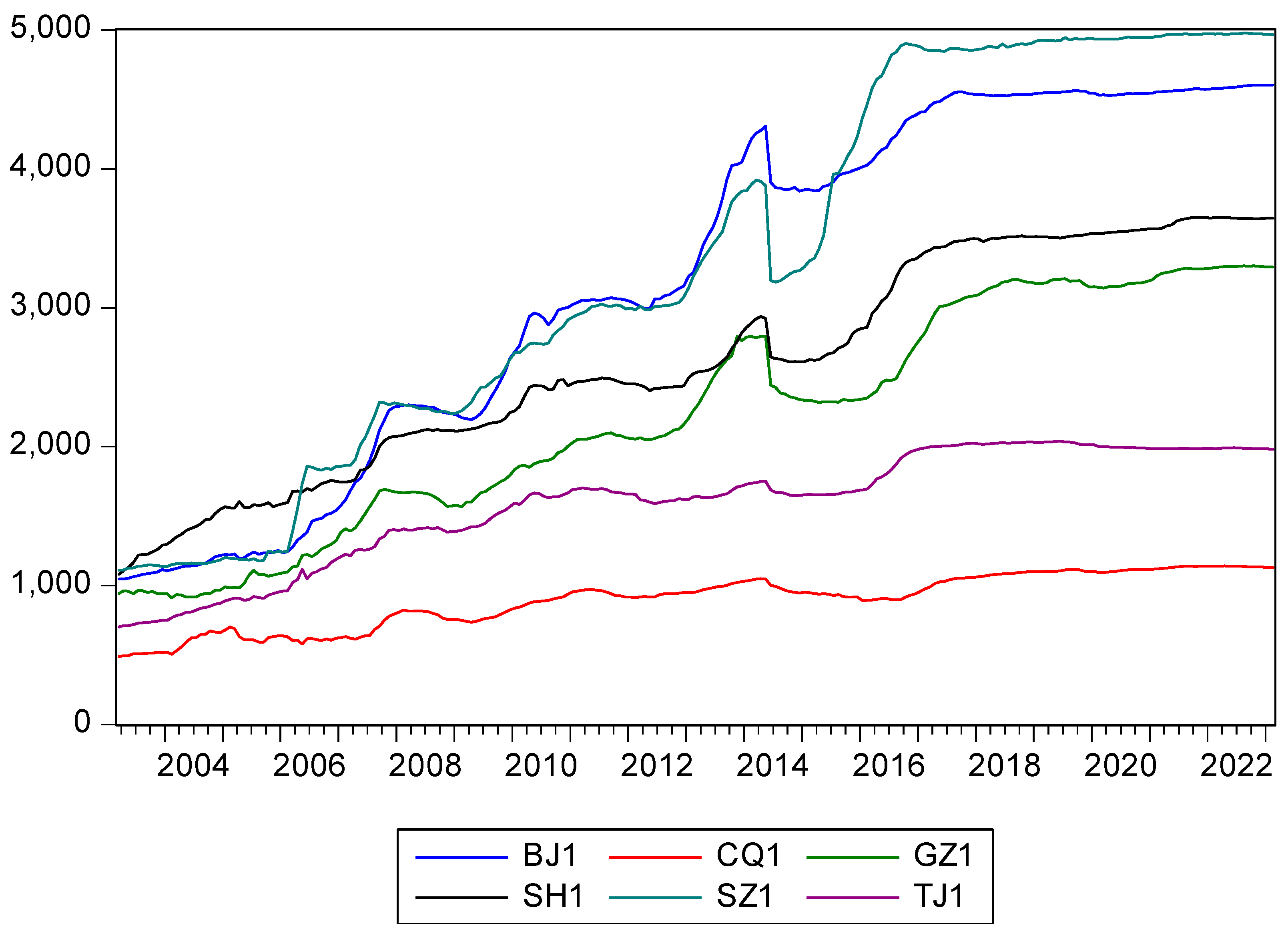
Mean	3202.787	894.6708	2219.500	2610.208	3321.000	1586.246
Median	3302.500	937.0000	2282.000	2533.500	3191.000	1657.000
Maximum	4606.000	1142.000	3303.000	3653.000	4978.000	2039.000
Minimum	1046.000	487.0000	911.0000	1080.000	1111.000	703.0000
Std. Dev.	1273.626	192.6036	801.4528	774.0704	1387.401	404.5648
	$X_{BJ}^O$	$X_{CQ}^O$	$X_{GZ}^O$	$X_{SH}^O$	$X_{SZ}^O$	$X_{TJ}^O$
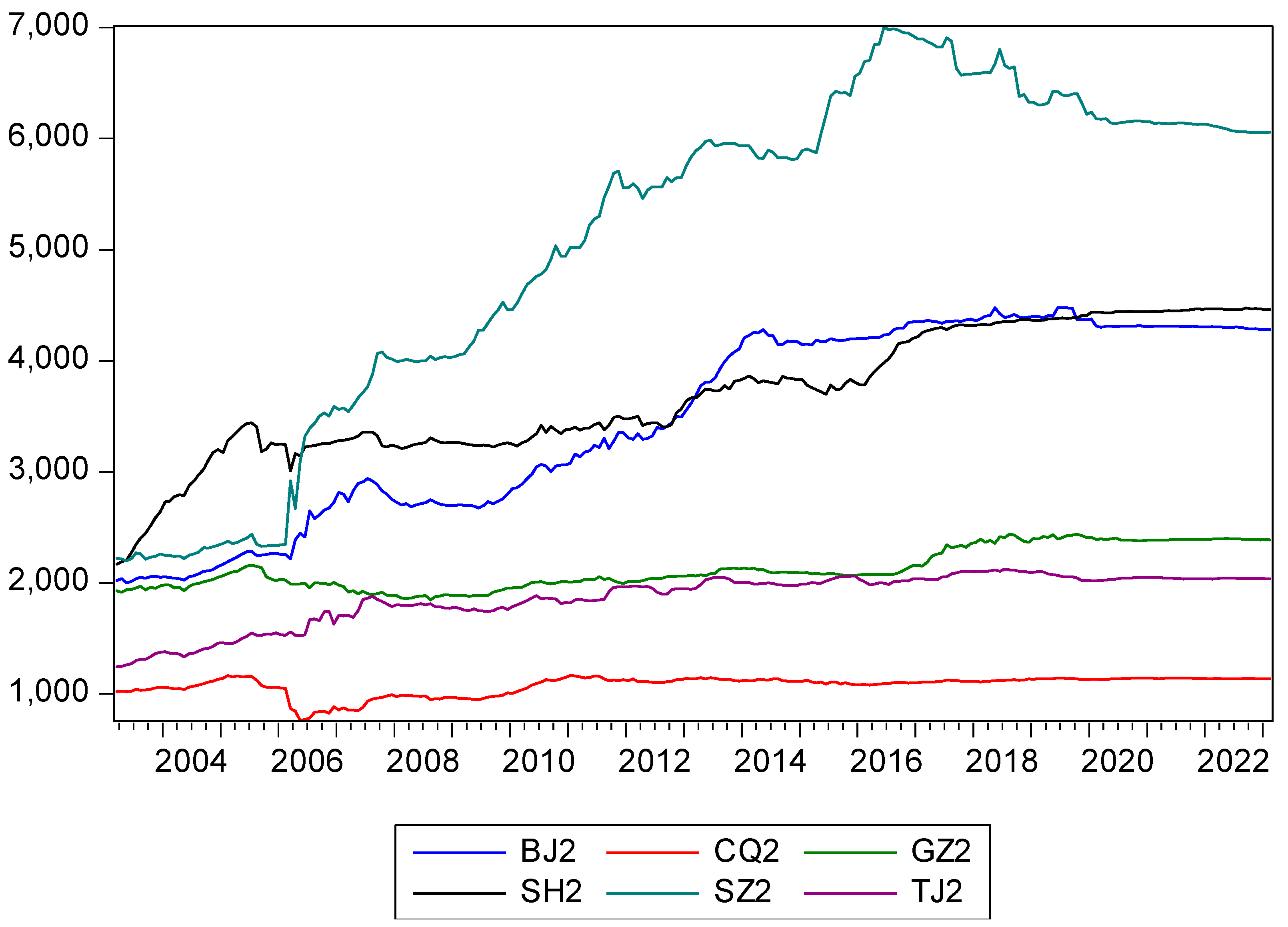
Mean	3482.354	1077.275	2123.221	3693.671	5065.242	1865.2
Median	3649	1115	2074	3663	5814.5	1971
Maximum	4479	1165	2439	4474	7004	2122
Minimum	2000	761	1846	2167	2196	1245
Std. dev.	857.08	85.917	183.877	572.51	1521.7	230.297
	$X_{BJ}^C$	$X_{CQ}^C$	$X_{GZ}^C$	$X_{SH}^C$	$X_{SZ}^C$	$X_{TJ}^C$
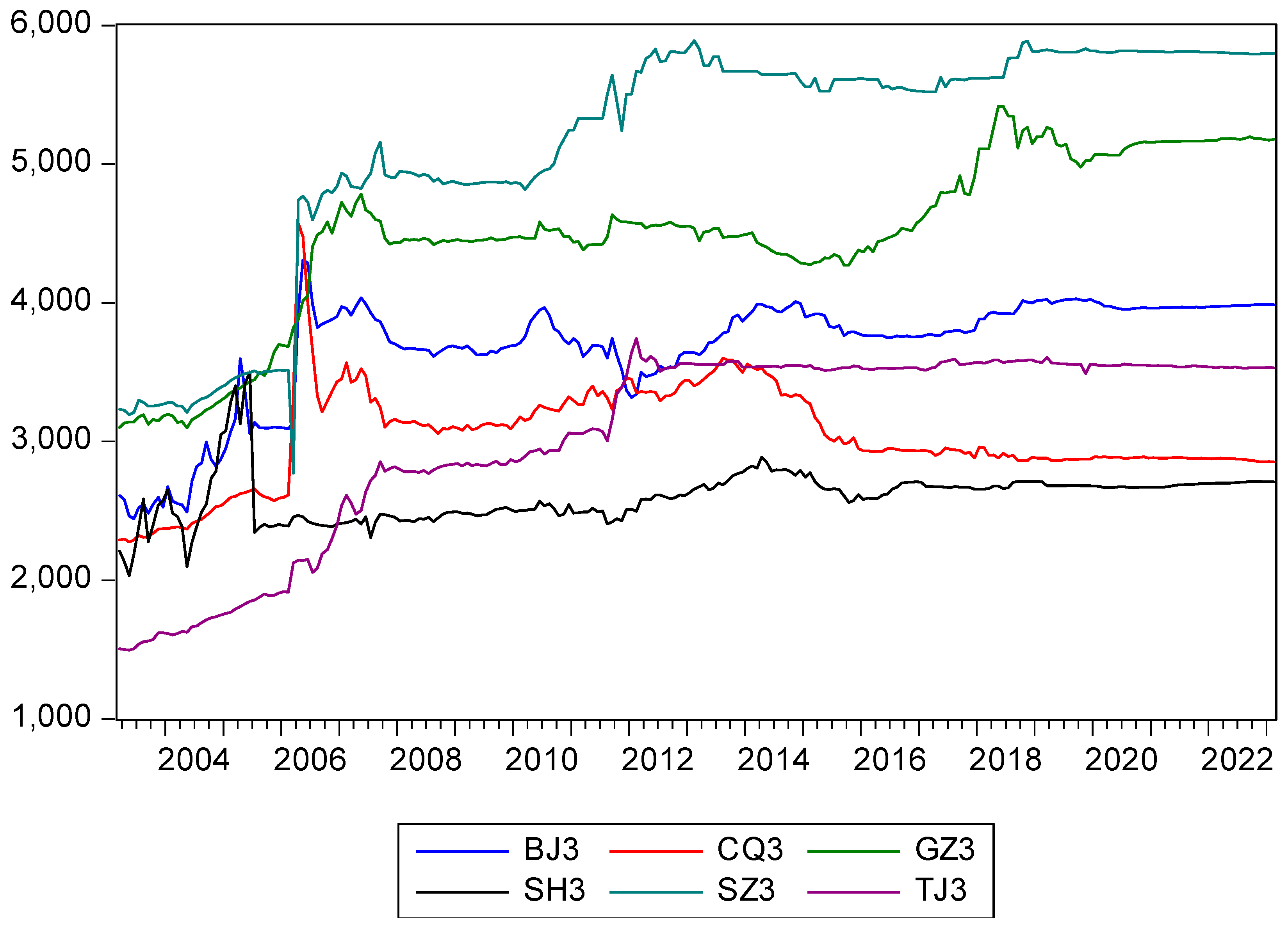
Mean	3678.427	3035.433	4481.642	2601.735	5134.871	3049.521
Median	3786	2952	4496	2651.25	5553	3526
Maximum	4309	4572	5416	3501.5	5891	3743
Minimum	2442	2275	3099	2031.5	2771	1495
Std. dev.	403.346	351.472	593.003	184.192	845.373	680.339

Source: CREIS database.

, it is found that SZ is the highest-price-risk city for all three submarkets, and BJ has the highest risk in its housing market.

We applied used Figure 2, Figure 3 and Figure 4 to show the trends in residential, office and retail real estate prices, respectively. It is clear that increases in residential prices with a strong co-movement are far higher than ones in commercial real estate prices. These results can fully prove that an overheated housing market exists in the case of six China’s cities.

Finally, whether all variables are I(1) or not is critical to the choice between a pure VAR and the ECM; thus, we applied the augmented Dickey–Fuller (ADF) test, which is the most popular method used to examine unstable data. Every series was verified using the ADF test with the null hypothesis that a unit root exists. Under the null hypothesis, it is found that most variables were accepted, as shown in

Table 2. ADF tests results for different real estate prices in the six cities.

	$\mathsf{\tau }$	${\mathsf{\tau }}_{\mathit{\mu }}$	${\mathsf{\tau }}_{\mathit{\tau }}$
$ln{X}_{BJ}^R$	2.577	−2.642 *	−0.623
$ln{X}_{CQ}^R$	2.023	−2.229	−2.399
${lnX}_{GZ}^R$	2.795	−1.715	−1.277
${lnX}_{SH}^R$	4.046	−3.661 ***	−2.767
$ln{X}_{SZ}^R$	2.524	−1.922	−1.284
${lnX}_{TJ}^R$	2.995	−3.994 ***	−1.873
${lnX}_{BJ}^O$	2.439	−2.169	−0.839
$ln{X}_{CQ}^O$	0.252	−2.200	−2.719
${lnX}_{GZ}^O$	1.325	−0.643	−1.845
$ln{X}_{SH}^O$	3.796	−4.619 ***	−5.066 ***
${lnX}_{SZ}^O$	1.866	−2.418	−1.025
${lnX}_{TJ}^O$	2.529	−3.688 ***	−2.497
$ln{X}_{BJ}^C$	1.180	−3.329 ***	−3.239 *
${lnX}_{CQ}^C$	0.504	−2.632 *	−2.547
$ln{X}_{GZ}^C$	2.721	−2.661 *	−1.869
${lnX}_{SH}^C$	0.336	−4.764 ***	−5.211 ***
${lnX}_{SZ}^C$	−1.593	−2.420	−1.945
$ln{X}_{TJ}^C$	2.831	−3.674 ***	−1.600
$∆ln{X}_{BJ}^R$	−4.334 ***	−6.094 ***	−8.712 ***
$∆{lnX}_{CQ}^R$	−10.132 ***	−10.419 ***	−10.535 ***
${∆lnX}_{GZ}^R$	−6.975 ***	−7.655 ***	−11.570 ***
$∆{lnX}_{SH}^R$	−5.370 ***	−11.197 ***	−11.781 ***
${∆lnX}_{SZ}^R$	−8.808 ***	−9.307 ***	−9.437 ***
$∆ln{X}_{TJ}^R$	−6.400 ***	−7.248 ***	−8.204 ***
$∆{lnX}_{BJ}^O$	−5.549 ***	−6.150 ***	−6.501 ***
$∆ln{X}_{CQ}^O$	−7.986 ***	−7.975 ***	−7.958 ***
$∆ln{X}_{GZ}^O$	−8.572 ***	−8.689 ***	−8.680 ***
${∆lnX}_{SH}^O$	−13.328 ***	−14.033 ***	−14.494 ***
${∆lnX}_{SZ}^O$	−5.557 ***	−5.930 ***	−6.367 ***
${∆lnX}_{TJ}^O$	−14.182 ***	−14.524 ***	−14.953 ***
$∆{lnX}_{BJ}^C$	−11.541 ***	−11.617 ***	−11.723 ***
${∆lnX}_{CQ}^C$	−10.533 ***	−10.531 ***	−10.661 ***
${∆lnX}_{GZ}^C$	−4.959 ***	−5.176 ***	−14.083 ***
$∆ln{X}_{SH}^C$	−8.557 ***	−8.553 ***	−8.553 ***
${∆lnX}_{SZ}^C$	−11.748 ***	−14.893 ***	−15.024 ***
${∆lnX}_{TJ}^C$	−11.392 ***	−11.947 ***	−12.645 ***

Notes: $\tau$, ${\tau }_{\mu }$, and ${\tau }_{\tau }$ represent the random walk, random walk with drift and random walk with a constant and time trend, respectively. *** and * represent 1% and 10% statistical significance, respectively. The numbers in parentheses are the lags calculated based on the Schwartz information criterion.

. At the same time, all first-differenced variables were rejected. Thus, all real estate prices belong to I(1) variables, and, hence, d = 1 in a LA-VAR model.

4.2. Real Estate Development in the Six Mega-Cities

To fully understand China’s real estate market, the six mega-cities were carefully chosen. The spatial distribution of the six cities is shown in Figure 5. From this figure, it can be seen that BJ and TJ are the twin cities located in the North, SH is located in the East, CQ is located in the West, and GZ and SZ are located in the South. Moreover, BJ, TJ, SH and CQ are four directly-controlled cities, meaning that these cities are directly controlled by the State Council (central government). Moreover, BJ, SH, GZ, and SZ are all first-tier cities, meaning that they can be regarded as fairly representative of China’s real estate market. More importantly, it is generally agreed that the overheating of the Chinese real estate market initially stemmed from these mega-cities. Examining these six cities is, therefore, very useful in investigating China’s real estate market.

As far as real estate investment in these cities is concerned, it is obvious from

Table 3. Distribution of real estate properties in the six cities.

	BJ		CQ		GZ		SH		SZ		TJ
Types	A	B	A	B	A	B	A	B	A	B	A	B
2003	0.756	0.244	0.739	0.261	0.828	0.172	0.834	0.166	0.801	0.199	0.825	0.175
2004	0.733	0.267	0.747	0.253	0.793	0.207	0.847	0.153	0.757	0.243	0.799	0.201
2005	0.716	0.284	0.772	0.228	0.762	0.238	0.818	0.182	0.766	0.234	0.814	0.186
2006	0.661	0.339	0.821	0.179	0.738	0.262	0.749	0.251	0.768	0.232	0.84	0.16
2007	0.661	0.339	0.85	0.15	0.783	0.217	0.726	0.274	0.799	0.201	0.777	0.223
2008	0.696	0.304	0.87	0.13	0.79	0.21	0.702	0.298	0.801	0.199	0.806	0.194
2009	0.712	0.288	0.85	0.15	0.729	0.271	0.711	0.289	0.766	0.234	0.792	0.208
2010	0.717	0.283	0.868	0.132	0.678	0.322	0.724	0.276	0.758	0.242	0.734	0.266
2011	0.729	0.271	0.842	0.158	0.723	0.277	0.753	0.247	0.777	0.223	0.706	0.294
2012	0.711	0.289	0.807	0.193	0.702	0.298	0.723	0.277	0.802	0.198	0.778	0.222
2013	0.65	0.35	0.797	0.203	0.718	0.282	0.684	0.316	0.799	0.201	0.788	0.212
2014	0.628	0.372	0.775	0.225	0.658	0.342	0.635	0.365	0.767	0.233	0.767	0.233
2015	0.581	0.419	0.745	0.255	0.713	0.287	0.618	0.382	0.748	0.252	0.778	0.222
2016	0.619	0.381	0.727	0.273	0.701	0.299	0.618	0.382	0.652	0.348	0.809	0.191
2017	0.606	0.394	0.761	0.239	0.738	0.262	0.652	0.348	0.536	0.464	0.847	0.153
2018	0.708	0.292	0.818	0.182	0.757	0.243	0.659	0.341	0.583	0.417	0.901	0.099
2019	0.761	0.239	0.835	0.165	0.769	0.231	0.669	0.331	0.608	0.392	0.906	0.094
2020	0.808	0.192	0.856	0.144	0.771	0.229	0.635	0.365	0.634	0.366	0.902	0.098
2021	0.836	0.164	0.869	0.131	0.811	0.189	0.676	0.324	0.631	0.369	0.899	0.101

Note: The commercial market comprises office and retail property. A and B represent residential and commercial property, respectively. Sources: The NBS.

that the commercial real estate markets in BJ, SH, and GZ, which account for more than 30% of the overall real estate investment, deserved more attention than the other cities. These three cities are not only first-tier cities, but also international metropolises. More importantly, this table shows that commercial real estate accounts for a substantial part of the urban real estate market in these cities.

5. Estimation Results and Policy Considerations

In this section, we present the results of the ripple effects for the three types of property by means of the ECM and causality tests. We then discuss the policy implications of these results and offer suggestions.

5.1. Long-Run Equilibrium and the ECM: Evidence of Ripple Effects

As stated in Section 3.2, a long-run equilibrium can ensure the availability and feasibility of the ripple effect; thus, we should try to determine whether a long-run equilibrium exists by performing cointegration analysis using the ECM, as shown in

Table 4. Model specification.

r	Specification 1	Specification 2	Specification 3
Residential form
0	199.895 ***	183.540 ***	197.246 ***
1	124.355 ***	114.417 ***	125.583 ***
2	77.283 ***	70.212 ***	80.591 ***
3	35.716 ***	31.160 **	41.462
Office form
0	157.532 ***	147.178 ***	159.189 ***
1	89.407 ***	82.628 ***	94.339 ***
2	54.588 **	47.946 ***	55.102
3	29.343	22.945	31.101
Retail form
0	153.456 ***	140.669 ***	170.321 ***
1	98.705 ***	91.718 ***	118.180 ***
2	63.140 ***	57.226 ***	74.410 ***
3	34.337 *	31.530 **	37.202

Note: r is the number of cointegration relationships. For critical values, the interested reader can refer to [85]. ***, ** and * represent 1%, 5% and 10% statistical significance, respectively.

. First, the lags are specified according to the lags of the first-differenced term in the auxiliary regression, and on the basis of the HQ criterion: the lag order is equal to one for the residential and retail markets, while the lag is six in the office market. Secondly, our cointegration estimation, based on Johansen’s [84] maximum likelihood method, is followed by two steps. We first select the best model specification based on the Pantula principle, with the joint hypothesis of both the rank order and deterministic components, to detect the number of cointegrating vectors being less than or equal to r cointegration relationships. As shown in Table 3, it is also clear that there are long-run equilibrium relationships in the residential, office and retail submarkets; thus, we can confirm that the ripple effect prevails over all three submarkets.

5.2. Ripple Effects across the Six Cities in the Three Submarkets

Table 5. Results of TY causality tests for the residential markets.

	Outcomes	BJ	CQ	GZ	SH	SZ	TJ
Causes
BJ			2.082	4.950 *	5.479 *	0.241	13.868 ***
CQ		2.136		8.169 ***	0.322	10.841 ***	14.007 ***
GZ		10.407 ***	4.034		0.136	1.477	19.965 ***
SH		7.429 **	1.729	1.225		0.673	5.898 ***
SZ		2.118 *	0.593	0.559	1.483		2.338
TJ		1.870	4.272	1.549	2.748	1.001
Abbreviations		1. GZ → BJ 2. SH → BJ		4. BJ → GZ 5. CQ → GZ	6. BJ → SH	7. CQ → SZ	8. BJ → TJ 9. CQ → TJ
		3. SZ → BJ					10. GZ → TJ 11. SH → TJ
Conclusions		BJ $\leftrightarrow$ GZ (1 and 4); BJ $\leftrightarrow$ SH (2 and 6); SZ → BJ (3); CQ → GZ (5); CQ → SZ (7); BJ → TJ (8); CQ → TJ (9); GZ → TJ (10); SH → TJ (11)

Note: The 1%, 5% and 10% significance levels of ${\chi }^2(2)$ are 9.210, 5.991 and 4.605, respectively. ***, ** and * represent 1%, 5% and 10% statistical significance, respectively.

reports the results of the TY causality test for residential markets among China’s six major cities. The row is denoted by “outcomes”, and is affected by the column, which is designated as “causes”. For example, BJ is significantly caused by GZ; at the same time, GZ is significantly caused by BJ. This causality can formally be abbreviated as “BJ $\leftrightarrow$ GZ” in a reciprocal or bi-directional manner; namely, the co-movement between BJ and GZ. Similarly, BJ and SH are two cities that affect each other; this causality is abbreviated as “BJ $\leftrightarrow$ SH”. On the other hand, while SZ is not affected by BJ, BJ is significantly affected by SZ; this relationships can be presented as “SZ → BJ”, which is known as the ripple effect or uni-directional causality. To summarize, there are seven ripple effects and two co-movements among the six cities for the residential real estate market. For the source cities, residential prices in BJ and CQ are both found to significantly affect the residential prices in three other cities; hence, these two cities can be regarded as the sources of recent residential price appreciation. Finally, the residential market in CQ appears to be partly isolated from other cities due to there being no evidence of a ripple effect and co-movement.

From

Table 6. Results of the TY causality test for the office markets.

	Outcomes	BJ	CQ	GZ	SH	SZ	TJ
Causes
BJ			2.082	3.950	5.479 *	0.241	40.48 ***
CQ		2.136		8.169 ***	0.322	10.84 ***	14.001 ***
GZ		10.407 ***	4.034		0.131	1.447	19.965 ***
SH		2.327	1.729	1.225		0.673 *	5.898 **
SZ		2.118	0.593	0.559	1.483		2.338
TJ		1.870	4.270	1.549	2.748	1.001
Abbreviations		1. GZ → BJ		2.CQ → GZ	3. BJ → SH	4. CQ → SZ 5. SH → SZ	6. BJ → TJ 7. CQ → TJ 8. GZ → TJ 9. SH → TJ
Conclusions		All are uni-directional causalities

Note: The 1%, 5% and 10% significance levels of ${\chi }^2(2)$ are 9.210, 5.991 and 4.605, respectively. ***, ** and * represent 1%, 5% and 10% statistical significance, respectively.

, we can see that the office market is different to the residential market. Firstly, there are no co-movements in the office market. Secondly, there are seven ripple effects among the six cities. It is, therefore, concluded that CQ is at the center of the ripple effects from the office market, with three ripple effects arising from this city. As far as the retail market is concerned, as shown in

Table 7. Results of the TY causality test for the retail markets.

	Outcomes	BJ	CQ	GZ	SH	SZ	TJ
Causes
BJ			0.283	2.716	1.137	7.471 **	0.835
CQ		4.367		5.942 *	0.093	6.818 ***	27.750 ***
GZ		1.920	0.922		0.172	0.410	1.420
SH		2.970	0.081	4.412		3.921	0.006
SZ		38.792 ***	1.102	0.512	13.819 ***		15.775 ***
TJ		1.012	10.770 ***	0.276	2.566	1.138
Abbreviations		1. SZ → BJ	2.TJ → CQ	3. CQ → GZ	4. SZ → SH	5. BJ → SZ 6. CQ → SZ	7. CQ → TJ 8. SZ → TJ
Conclusions		BJ $\leftrightarrow$ SZ (1 and 5); CQ $\leftrightarrow$ TJ (2 and 7); CQ → GZ (3); SZ → SH (4); CQ → SZ (6); SZ → TJ (8)

Note: The 1%, 5% and 10% significance levels of ${\chi }^2(2)$ are 9.210, 5.991 and 4.605, respectively. ***, ** and * represent 1%, 5% and 10% statistical significance, respectively.

, there are two bi-directional relationships between BJ and SZ. In addition, there are four ripple effects among the six cities. Moreover, the ripple effects in the retail market mainly stem from SZ and CQ; the retail market in SH is almost isolated from the other five cities.

As can be seen from the above, there are apparent differences in the ripple effects affecting the three types of property for interconnected networks; these findings are also summarized in

Table 8. Summary of ripple effects in the three submarkets.

	Sources	Number of Causalities	Bi-Directional (Co-Movement)	Uni-Directional (Ripple Effects)
Housing	BJ and CQ	11	2	7
Office	CQ	9	0	9
Retail	SZ and CQ	8	2	4

. Firstly, the scale of funding for commercial real estate is far larger than that for housing; the former is dominated by institutional investors, while the latter is mainly transacted by households or individuals. Consequently, the price of commercial real estate must be appraised rationally and professionally, while the price of housing is often unreasonably high or low due to the psychological level of the public, which gives rise to inter-regional ripple effects [86,87]. Secondly, commercial real estate is further divided into office and retail types; the retail market serves local consumers, while the office market must communicate with national and global clients. Therefore, the retail market almost completely relies on the local economy, while the health of the office market is related to both national and global leakages.

5.3. Policy Implications

Over the past few decades, while a great deal of effort has been made to assess the ripple effects among local housing markets, little attention has been paid to the ripple effects in other real estate property markets. In this study, the long-run equilibrium relationships in all three property submarkets proved the existence of such ripple effects for housing, office and retail assets. Secondly, we found that there were diverse ripple effects at work in the residential, office and retail markets in China. The results clearly show that it is imperative to consider the ripple effects in these three property submarkets. Thirdly, there were different source cities for different types of property based on ripple effects (BJ and CQ in the residential market, and SZ and CQ in the office and retail markets).

Since we know the individual source cities for the three different property markets, portfolio management seems to be a noteworthy approach that encourages excess capital to move from the residential market to the commercial market, according to the respective source cities. To accelerate the flow of capital, we argue that the ripple effects from the source cities are very useful to efficiently promoting an appropriate level of diversification planning. In an overheated residential market, the authorities can exercise a housing price control policy in BJ and CQ, to transmit “negative” ripple effects to other cities, thus dampening housing price appreciation. In contrast, incentive policies related to commercial real estate can be introduced in SZ and CQ in advance, to speed up the transfer of positive ripple effects to other cities and, hence, growing commercial markets. Based on the above steps, a stable and balanced real estate portfolio based on diversification can be set up to fight against the shocks from a specific type of property, such as housing or commercial real estate assets.

Beyond the diversification strategy, some critical national policies also deserve emphasis. For example, a new policy that allows the public to invest in commercial real estate by buying Real Estate Investment Trusts (REITs), can be trialed in SZ as a pilot city; if successful, the REIT system can be extended to other cities. Finally, we also argue that China’s expansionary monetary policy should promptly guide and channel excess liquidity from residential to commercial property markets through the People’s Bank of China (PBC) [13,14].

In summary, we propose a diversification strategy to set up a reliable real estate portfolio among housing office and retail markets through ripple effects and source cities. At the same time, macroeconomic policies, such as the development of REITs and the guidance from monetary policy, must be accompanied. Once an effective diversification strategy is implemented, we believe that real estate market sustainability in China can be come a reality in the near future.

6. Conclusions

Very high housing prices and possible price bubbles in China have recently become a severe economic and political problem. To comprehensively understand and resolve this issue by means of diversification and portfolio theory, we examined the individual ripple effects in three property markets (the residential, office and retail property markets) to identify their source cities associated with the opposite policy proposals. Thus, this paper is different from the past studies for two reasons. The first reasons is that we estimated kinds of ripple effects from housing, office and retail markets, respectively; past studies largely focused only on the housing market across various cities. The second point is that we proposed differentiated policies for the housing market (control policy) and the commercial market (incentive policy) in the corresponding source cities, to more efficiently dampen the overheated housing market and to encourage commercial real estate market development. By completing this diversification strategy is completed, we can increase the Chinese real estate market sustainability by excluding the disturbances caused by housing or commercial real estate markets.

The ECM results reveal that all three property submarkets point to long-run equilibrium relationships, on the grounds that ripple effects are found to promote equilibrium across cities in the long run. Moreover, the causality test was adopted to examine the lead-lag relationship in every property submarket. Our results fully indicate that ripple effects exist in China, but the spillover processes in the three property submarkets are very different. The sources of real estate property appreciation in the three submarkets are BJ and CQ (residential), CQ (office), and SZ and CQ (retail), respectively. Although the ripple effect in the housing market across cities is larger than that for commercial real estate, according to portfolio theory, a heated residential market and a sluggish commercial market should be managed differently: the authorities should impose controls over the residential market in source cities (BJ and CQ), which send negative information to other cities to shock against overheated housing markets; in contrast, the government should implement a promotion policy for the commercial market in its respective source cities (SZ and CQ), which then sends positive information to other cities to encourage the commercial market development. As long as this process is successful, a sustainable real estate market, through a balanced and stable real estate portfolio, can be built up.

Finally, we want to show two things: that limitations in data collection and time-series econometrics force us to concentrate on six mega-cities, and; that although we apply ECM and TY causality to assist the authorities to resolve overheated housing markets by diversifying various real estate assets, we must keep in mind that China is a changing economy. Thus, new time-varying econometrics, which are used to trace out the changes in ripple effects across residential, office and retail real estate markets, may provide worthwhile scope for future work to ensure effective management of real estate portfolios.

References

- Zhang, C.; An, G.; Yu, X. What drives China’s house prices: Marriage or money? China World Econ. 2012, 20, 19–36. [Google Scholar] [CrossRef]
- Yang, Z.; Chen, J. Housing Reform and the Housing Market in Urban China (Chapter 2) from Housing Affordability and Housing Policy in Urban China; Springer: Berlin, Germany, 2014. [Google Scholar]
- Hui, E.C.M.; Chan, K.K.K. Foreign direct investment in China’s real estate market. Habitat Int. 2014, 43, 231–239. [Google Scholar] [CrossRef]
- Chen, J.; Guo, F.; Wu, Y. One decade of urban housing reform in China: Urban housing price dynamics and the role of migration and urbanization, 1995–2005. Habitat Int. 2011, 35, 1–8. [Google Scholar] [CrossRef]
- Ofori, G.; Han, S. Testing hypotheses on construction and development using data on China’s provinces, 1990–2000. Habitat Int. 2003, 27, 37–62. [Google Scholar] [CrossRef]
- Chen, J.; Guo, F.; Zhu, A. The housing-led growth hypothesis revisited: Evidence from the Chinese provincial panel data. Urban Stud. 2011, 48, 2049–2067. [Google Scholar] [CrossRef]
- Kong, Y.; Glascock, J.L.; Lu-Andrews, R. An investigation into real estate investment and economic growth in China: A dynamic panel data approach. Sustainability 2016, 8, 66. [Google Scholar] [CrossRef] [Green Version]
- Wu, J.; Gyourko, J.; Deng, Y. Evaluating conditions in major Chinese housing markets. Reg. Sci. Urban Econ. 2012, 42, 531–543. [Google Scholar] [CrossRef] [Green Version]
- Glaeser, E.; Huang, W.; Ma, Y.; Shleifer, A. A real estate boom with Chinese characteristics. J. Econ. Perspect. 2017, 31, 93–116. [Google Scholar] [CrossRef] [Green Version]
- Weng, Y.; Gong, P. On price co-movement and volatility spillover effects in China’s housing markets. Int. J. Strateg. Prop. Manag. 2017, 21, 240–255. [Google Scholar] [CrossRef] [Green Version]
- Chen, C.; Chiang, S. Time-varying spillovers among first-tier housing markets in China. Urban Stud. 2020, 57, 844–864. [Google Scholar] [CrossRef]
- Tan, Z.; Tang, Q.; Meng, J. The effect of monetary policy on China’s housing prices before and after 2017: A dynamic analysis in DSGE model. Land Use Policy 2022, 113, 105927. [Google Scholar] [CrossRef]
- Zhang, C. Money, housing and inflation in China. J. Policy Model. 2013, 35, 75–87. [Google Scholar] [CrossRef]
- Chiang, S. Rising residential rents in Chinese mega cities: The role of monetary policy. Urban Stud. 2016, 53, 3493–3509. [Google Scholar] [CrossRef]
- Toda, H.Y.; Yamamoto, T. Statistical inference in vector autoregressions with possibly integrated processes. J. Econom. 1995, 66, 225–250. [Google Scholar] [CrossRef]
- Giussani, B.; Hadjimatheou, G. Modelling regional house prices in the UK. Pap. Reg. Sci. 1991, 70, 201–219. [Google Scholar] [CrossRef]
- MacDonald, R.; Taylor, M. Regional house prices in Britain: Long-run relationships and short-run dynamics. Scott. J. Political Econ. 1993, 40, 43–55. [Google Scholar] [CrossRef]
- Drake, L. Testing for convergence between UK regional house prices. Reg. Stud. 1995, 29, 357–366. [Google Scholar] [CrossRef]
- Alexander, C.; Barrow, M. Seasonality and cointegration of regional house prices in the UK. Urban Stud. 1994, 31, 1667–1689. [Google Scholar] [CrossRef]
- Holly, S.; Pesaran, H.; Yamagata, T. The spatial and temporal diffusion of house prices in the UK. J. Urban Econ. 2011, 69, 2–23. [Google Scholar] [CrossRef] [Green Version]
- Cascio, I.L. A wavelet analysis of the ripple effect in UK regional housing markets. Int. Rev. Econ. Financ. 2021, 76, 1093–1105. [Google Scholar] [CrossRef]
- Luo, Z.; Liu, C.; Picken, D. Housing price diffusion pattern of Australia’s state capital cities. Int. J. Strateg. Prop. Manag. 2007, 11, 227–242. [Google Scholar] [CrossRef] [Green Version]
- Liu, C.; Luo, Z.Q.; Ma, L.; Picken, D. Identifying house price diffusion patterns among Australian state capital cities. Int. J. Strateg. Prop. Manag. 2008, 12, 237–250. [Google Scholar] [CrossRef] [Green Version]
- Shi, S.; Young, M.; Hargreaves, B. The ripple effect of local house price movements in New Zealand. J. Prop. Res. 2009, 26, 1–24. [Google Scholar] [CrossRef]
- Hurn, S.; Shi, S.; Wang, B. Housing networks and driving forces. J. Bank. Financ. 2022, 134, 106318. [Google Scholar] [CrossRef]
- Lee, C.; Chien, M. Empirical modeling of regional house prices and the ripple effect. Urban Stud. 2011, 48, 2029–2047. [Google Scholar] [CrossRef]
- Chen, P.; Chien, M.; Lee, C. Dynamic modeling of regional house price diffusion in Taiwan. J. Hous. Econ. 2011, 20, 315–332. [Google Scholar] [CrossRef]
- Chien, M. Structural breaks and the convergence of regional house prices. J. Real Estate Financ. Econ. 2010, 40, 77–88. [Google Scholar] [CrossRef]
- Balcilar, M.; Beyene, A.; Gupta, R.; Seleteng, M. ‘Ripple’ effects in South African house prices. Urban Stud. 2013, 50, 876–894. [Google Scholar] [CrossRef] [Green Version]
- Gupta, R.; André, C.; Gil-Alana, L. Comovement in Euro area housing prices: A fractional cointegration approach. Urban Stud. 2014, 51, 3123–3143. [Google Scholar] [CrossRef] [Green Version]
- Helgers, R.; Buyst, E. Spatial and temporal diffusion of housing prices in the presence of a linguistic border: Evidence from Belgium. Spat. Econ. Anal. 2016, 11, 92–122. [Google Scholar] [CrossRef]
- Teye, A.L.; Ahelegbey, D.F. Detecting spatial and temporal house price diffusion in the Netherlands: A Bayesian network approach. Reg. Sci. Urban Econ. 2017, 65, 56–64. [Google Scholar] [CrossRef] [Green Version]
- Gupta, R.; Miller, S.S. “Ripple effects” and forecasting home prices in Los Angeles, Las Vegas and Phoenix. Ann. Reg. Sci. 2012, 48, 763–782. [Google Scholar] [CrossRef] [Green Version]
- Yunus, N.; Swanson, P.E. A closer look at the U.S. housing market: Modeling relationships among regions. Real Estate Econ. 2013, 41, 542–568. [Google Scholar] [CrossRef]
- Cohen, J.P.; Zabel, J. Local house price diffusion. Real Estate Econ. 2020, 48, 710–743. [Google Scholar] [CrossRef]
- Tsai, I. Features of the ripple effect in the US regional housing markets: A viewpoint of nonsynchronous trading. Int. J. Urban Sci. 2022, 26, 373–397. [Google Scholar] [CrossRef]
- Ranjbar, O.; Gholipour, H.F.; Saboori, B.; Chang, T. Tehran’s house price ripple effects in Iran: Application of bootstrap asymmetric panel Granger non-causality in the frequency domain. Hous. Stud. 2022, 37, 1566–1597. [Google Scholar] [CrossRef]
- Chiang, S. Housing markets in China and policy implications: Co-movement or ripple effect. China World Econ. 2014, 22, 103–120. [Google Scholar] [CrossRef]
- Lee, C.; Lee, C.; Chiang, S. Ripple effect and regional house prices dynamics in China. Int. J. Strateg. Prop. Manag. 2016, 20, 397–408. [Google Scholar] [CrossRef] [Green Version]
- Gong, Y.; Hu, J.; Boelhouwer, P.J. Spatial interrelations of Chinese housing markets: Spatial causality, convergence and diffusion. Reg. Sci. Urban Econ. 2016, 59, 103–117. [Google Scholar] [CrossRef]
- Zhang, F.; Morley, B. The convergence of regional house prices in China. Appl. Econ. Lett. 2014, 21, 205–208. [Google Scholar] [CrossRef] [Green Version]
- Mao, G. Do regional house prices converge or diverge in China? China Econ. J. 2016, 9, 154–166. [Google Scholar] [CrossRef]
- Chow, W.W.; Fung, M.K.; Cheng, A.C.S. Convergence and spillover of house prices in Chinese cities. Appl. Econ. 2016, 48, 4922–4941. [Google Scholar] [CrossRef]
- Xiao, Q. Equilibrating ripple effect, disturbing information cascade effect and regional disparity—A perspective from China’s tiered housing markets. Int. J. Financ. Econ. 2023, 28, 858–878. [Google Scholar] [CrossRef]
- Gyourko, J.; Linneman, P. Owner-occupied homes, income-producing properties and REITs as inflation hedges: Empirical findings. J. Real Estate Financ. Econ. 1988, 1, 347–372. [Google Scholar] [CrossRef]
- Wheaton, W.C. Real estate “Cycles”: Some fundamentals. Real Estate Econ. 1999, 27, 209–230. [Google Scholar] [CrossRef]
- Ghebreegziabiher, D.; Pels, E.; Rietveld, P. The impact of railway stations on residential and commercial property value: A meta-analysis. J. Real Estate Financ. Econ. 2007, 35, 161–180. [Google Scholar]
- Davis, M. The price and quantity of land by legal form of organization in the United States. Reg. Sci. Urban Econ. 2009, 39, 350–359. [Google Scholar] [CrossRef]
- Nichols, J.B.; Onliner, S.D.; Mulhall, M.R. Swings in commercial and residential land prices in the United States. J. Urban Econ. 2013, 73, 57–76. [Google Scholar] [CrossRef]
- Gyourko, J. Understanding commercial real estate: How different from housing is it? J. Portf. Manag. 2009, 35, 23–37. [Google Scholar] [CrossRef]
- Hui, E.C.M.; Zheng, X. Exploring the dynamic relationship between housing and retail property markets: An empirical study of Hong Kong. J. Prop. Res. 2012, 29, 85–102. [Google Scholar] [CrossRef]
- Chiang, S. Interaction among real estate properties in China using three submarket panels. Habitat Int. 2016, 53, 243–253. [Google Scholar] [CrossRef]
- Kishor, N.K. Comovements and spillovers in international commercial and residential real estate markets. J. Eur. Real Estate Res. 2022, 15, 311–331. [Google Scholar] [CrossRef]
- Ibbotson, R.G.; Fall, C.L. The United States market wealth portfolio. J. Portf. Manag. 1979, 6, 82–92. [Google Scholar] [CrossRef]
- Gyourko, J.; Nelling, E. Systematic risk and diversification in the equity REIT market. Real Estate Econ. 1996, 24, 493–515. [Google Scholar] [CrossRef]
- Capozza, D.R.; Seguin, P.J. Managerial style and firm value. Real Estate Econ. 1998, 26, 131–150. [Google Scholar] [CrossRef] [Green Version]
- Chen, J.; Peiser, R. The risk and return characteristics of REITs. Real Estate Financ. 1999, 16, 61–68. [Google Scholar]
- Brown, R.J.; Li, L.; Lusht, K. A note on intracity geographic diversification of real estate portfolios: Evidence from Hong Kong. J. Real Estate Portf. Manag. 2000, 6, 131–140. [Google Scholar] [CrossRef]
- Chan, S.; Erickson, J.; Wang, K. Real Estate Investment Trust: Structure, Performance and Investment Opportunities; Oxford University Press: Oxford, UK, 2003. [Google Scholar]
- Hartzell, D.; Heckman, J.; Miles, M. Diversification categories in investment real estate. Real Estate Econ. 1986, 14, 230–254. [Google Scholar] [CrossRef]
- Clayton, J.; MacKinnon, G. The time-varying nature of the link between REIT, real estate and financial asset returns. J. Real Estate Portf. Manag. 2001, 7, 43–54. [Google Scholar] [CrossRef]
- Heston, S.L.; Rouwenhorst, G.K. Does industrial structure explain the benefits of international diversification? J. Financ. Econ. 1994, 36, 3–27. [Google Scholar] [CrossRef]
- Van Dijk, R.; Keijzer, T. Region, sector and style selection in global equity markets. J. Asset Manag. 2004, 4, 293–307. [Google Scholar] [CrossRef]
- Hamelink, F.; Hoesli, M. What factors determine international real estate security returns? Real Estate Econ. 2004, 32, 437–462. [Google Scholar] [CrossRef] [Green Version]
- Gallo, J.G.; Zhang, Y. Global property market diversification. J. Real Estate Financ. Econ. 2010, 41, 458–485. [Google Scholar] [CrossRef]
- De Wit, I. International diversification strategies for direct real estate. J. Real Estate Financ. Econ. 2010, 41, 433–457. [Google Scholar] [CrossRef]
- Clapp, J.M.; Tirtiroglu, D. Positive feedback trading and diffusion of asset price changes: Evidence from housing transactions. J. Econ. Behav. Organ. 1994, 24, 337–355. [Google Scholar] [CrossRef]
- Clapp, J.M.; Dolde, W.; Tirtiroglu, D. Imperfect information and investor inferences from housing price dynamics. Real Estate Econ. 1995, 23, 239–269. [Google Scholar] [CrossRef]
- Dolde, W.; Tirtiroglu, D. Temporal and spatial information diffusion in real estate price changes and variances. Real Estate Econ. 1997, 25, 539–565. [Google Scholar] [CrossRef]
- Fernando, F.; Gyourko, J. Heterogeneity in neighborhood-level price growth in the United States, 1993–2009. Am. Econ. Rev. 2012, 102, 134–140. [Google Scholar]
- DeFusco, A.; Ding, W.; Ferreira, F.; Gyourko, J. The role of price spillovers in the American housing boom. J. Urban Econ. 2018, 108, 72–84. [Google Scholar] [CrossRef]
- Zhu, E.; Wu, J.; Liu, H.; Li, X. Within-city spatial distribution, heterogeneity and diffusion of house price: Evidence from a spatiotemporal index for Beijing. Real Estate Econ. 2022, 50, 621–655. [Google Scholar] [CrossRef]
- Hu, J.; Xiong, X.; Cai, Y.; Yuan, F. The ripple effect and spatiotemporal dynamics of intra-urban housing prices at the submarket level in Shaghai, China. Sustainability 2020, 12, 5073. [Google Scholar] [CrossRef]
- Grigoryeva, I.; Ley, D. The price ripple effect in the Vancouver housing market. Urban Geogr. 2019, 40, 1168–1190. [Google Scholar] [CrossRef]
- Bangura, M.; Lee, C.L. House price diffusion of housing submarkets in Greater Sydney. Hous. Stud. 2020, 35, 1110–1141. [Google Scholar] [CrossRef]
- Kim, L.; Seo, W. Micro-analysis of price spillover effect among regional housing submarkets in Korea: Evidence from the Seoul metropolitan area. Land 2021, 10, 879. [Google Scholar] [CrossRef]
- Ho, L.; Ma, Y.; Haurin, D.R. Domino effects within a housing market: The transmission of house price changes across quality tiers. J. Real Estate Financ. Econ. 2008, 37, 299–311. [Google Scholar] [CrossRef]
- Brzezicka, J.; Laszek, J.; Olszewski, K.; Waszczuk, J. Analysis of the filtering process and the ripple effect on the primary and secondary housing market in Warsaw, Poland. Land Use Policy 2019, 88, 204098. [Google Scholar] [CrossRef]
- Markowitz, H.M. Portfolio selection. J. Financ. 1952, 7, 77–91. [Google Scholar]
- Meen, G.P. Regional house prices and the ripple effect: A new interpretation. Hous. Stud. 1999, 33, 425–444. [Google Scholar] [CrossRef]
- Hui, E.C.M.; Yue, S. Housing price bubbles in Hong Kong, Beijing and Shanghai: A comparative study. J. Real Estate Financ. Econ. 2006, 33, 299–327. [Google Scholar] [CrossRef]
- Tsai, I.; Chiang, S. Exuberance and spillovers in housing markets: Evidence from first- and second-tier cities in China. Reg. Sci. Urban Econ. 2019, 77, 75–86. [Google Scholar] [CrossRef]
- Chiang, S.; Hui, E.C.M.; Chen, C. Asymmetric housing information diffusions in China: An investor perspective. Urban Stud. 2022, 59, 2036–2052. [Google Scholar] [CrossRef]
- Johansen, S. Likelihood-based Inference in Cointegrated Vector Autoregressive Models; Oxford University Press: Oxford, UK, 1995. [Google Scholar]
- MacKinnon, J.G.; Haug, A.A.; Michelis, L. Numerical distribution functions of likelihood ratio tests for cointegration. J. Appl. Econom. 1999, 14, 563–577. [Google Scholar] [CrossRef]
- Black, A.; Fraser, P.; Hoesli, M. House prices, fundamentals and bubbles. J. Bus. Financ. Account. 2006, 33, 1535–1555. [Google Scholar] [CrossRef]
- Phillips, P.C.B.; Shi, S.; Yu, J. Specification sensitivity in right-tailed unit root testing for explosive behaviour. Oxf. Bull. Econ. Stat. 2014, 76, 315–333. [Google Scholar] [CrossRef]