Finite Frequency H_∞ Control for Doubly Fed Induction Generators with Input Delay and Gain Disturbance

Abstract

Due to the rapid development of wind power, the stable operation of doubly fed induction generators (DFIGs) has attracted much attention. This paper focuses on the finite frequency (FF) H_∞ control for the DFIG with input delay, aiming to reduce the effects of current harmonic interferences and gain disturbances on the DFIG and improve the stability of the system. First, a DFIG state–space model with input delay under current harmonics was constructed. Second, based on the DFIG state–space model, an FF H_∞ state-feedback controller was designed from the frequency domain perspective, which makes the DFIG stable and robust against harmonic interferences and gain disturbances. Third, via the generalized Kalman–Yakubovich–Popov (GKYP) lemma and the Lyapunov theory, the FF H_∞ performance was evaluated in the form of linear matrix inequalities (LMIs), and then the state feedback FF H_∞ controller was designed. Finally, the simulation results showed the efficiency of the proposed approach.

1. Introduction

With the heavy consumption of fossil fuels, the quick depletion of natural resources and the severe deterioration of the environment, the exploration and deployment of clean and renewable energies has become urgent for sustainable economies [1]. Wind energy has attracted global attention since it is recyclable and does not pollute the ecological environment [2]. Wind power has the advantages of a wide abundance of reserves, high utilization rates and small land occupation [3]. Due to the transmission protocol and transmission environment, the signal transmission of DFIGs usually produces a time delay. The time delay is always present in the control and feedback channels of wind turbines because of the time required for the feedback digital controller to calculate and transmit, as well as unpredictable events during transmission (slowing down of data transmission due to temperature variations and electromagnetic interference). Studies show that small delays may hamper the control effects and even destabilize wind turbine systems [4].

Among wind systems, doubly fed induction generators (DFIGs) are low-cost and high-efficiency by virtue of constant frequency and variable speed advantages, and they are the mainstream type of wind turbines at present. The power quality is strongly influenced by the wind power grid connection. (1) Power electronics used in DFIG systems may cause harmonic pollution and affect the power quality. (2) The randomness of the wind speed in the wind farm causes changes in the output power, resulting in inevitable fluctuations and flicker in the voltage. (3) The intermittent wind power may lead to severe grid frequency fluctuations, which affects the power quality. In DFIG-based wind farms, DFIGs cannot ignore time delay in their input. In [5], considering time delay uncertainties in wind turbines, a multi-delay stabilization via the Casimir function was developed. In [6], a compensator was installed to overcome time delay effects. In [7], in the small disturbance stability sense, wind power stabilization was constructed, and sufficient criteria were obtained.

Practical signals only have finite frequency features; for example, seismic waves emerge only in the frequency interval (0.3,8) Hz, while human acoustic perception is most sensitive over (4,8) Hz. By [8], finite frequency (FF) current harmonics are associated with the stator itself, rotor converter and grids. In [9], when three-phase grid voltages are unbalanced, the grids will generate stator negative sequence voltage and current. However, most control strategies for DFIGs are contrived commonly in the entire frequency (EF) domain sense [10]. This brings in high conservatism in controller parametrization, which leads to low robustness under FF harmonics.

To cope with the delay and gain disturbances, various control strategies are employed, including adaptive [11], sliding mode [12], model predictive [13], and $H_{\infty }$ optimal [14]. In particular, $H_{\infty }$ control has been intensively considered for wind turbines for stability robustness and disturbance attenuation. For practical DFIGs, the limitation of microprocessor memory and word length, as well as A/D and D/A conversion errors, may cause the control to be inaccurate. This gain disturbance can easily lead to the destruction of the closed-loop system stability and performance degradation. Though remarkable theories have been established in the FF sense, few works are specified for DFIGs. Therefore, it is still substantial and challenging to deal with DFIG control in the FF sense.

This paper addresses the H_∞ control for a single DFIG with input delay under FF current harmonics interference and gain disturbance. More precisely, the H_∞ index is used to evaluate current harmonics and gain disturbance. By exploiting the generalized Kalman–Yakubovich–Popov(GKYP) lemma, the performance indices are converted into LMIs, and controller parametrization is solved by means of LMI feasible solution. In brief, this study contributes a novel type of FF control for the wind turbine DFIG with input delay under controller gain disturbances and current harmonics. Through the GKYP lemma and the Lyapunov theory, the FF H_∞ performance is transformed into linear matrix inequalities (LMIs) to facilitate the design of FF controllers with input delay. It has not been fully considered in previous studies on the control of the wind turbine DFIG. Moreover, a sufficient condition is presented to design the optimal FF controller for the DFIG.

The suggested H_∞ control improves robustness against time delay and gain disturbances, in comparison to those by EF control ones.

Notations: For a matrix $M$, its transpose, inverse and orthogonal complements are denoted by $M^T$, $M^{-1}$ and $M^{\perp }$, respectively. $M^H={\overline{M}}^T$ means conjugate transpose. $M^T=M>0$ means that the symmetric matrix $M$ is positive. Given a square matrix $P$, $\mathrm{He}(P)=P+P^T$. $I_n$ denotes the $n\times n$ identity matrix. $R$ and $C$ denote the real and complex number sets, respectively. $R^{n\times m}$ and $C^{n\times m}$ denote the set of all real and complex matrices of dimension $n\times m$, respectively. Also, ∗ denotes the transposed element in the symmetric position.

2. Preliminaries and Problem Formulation

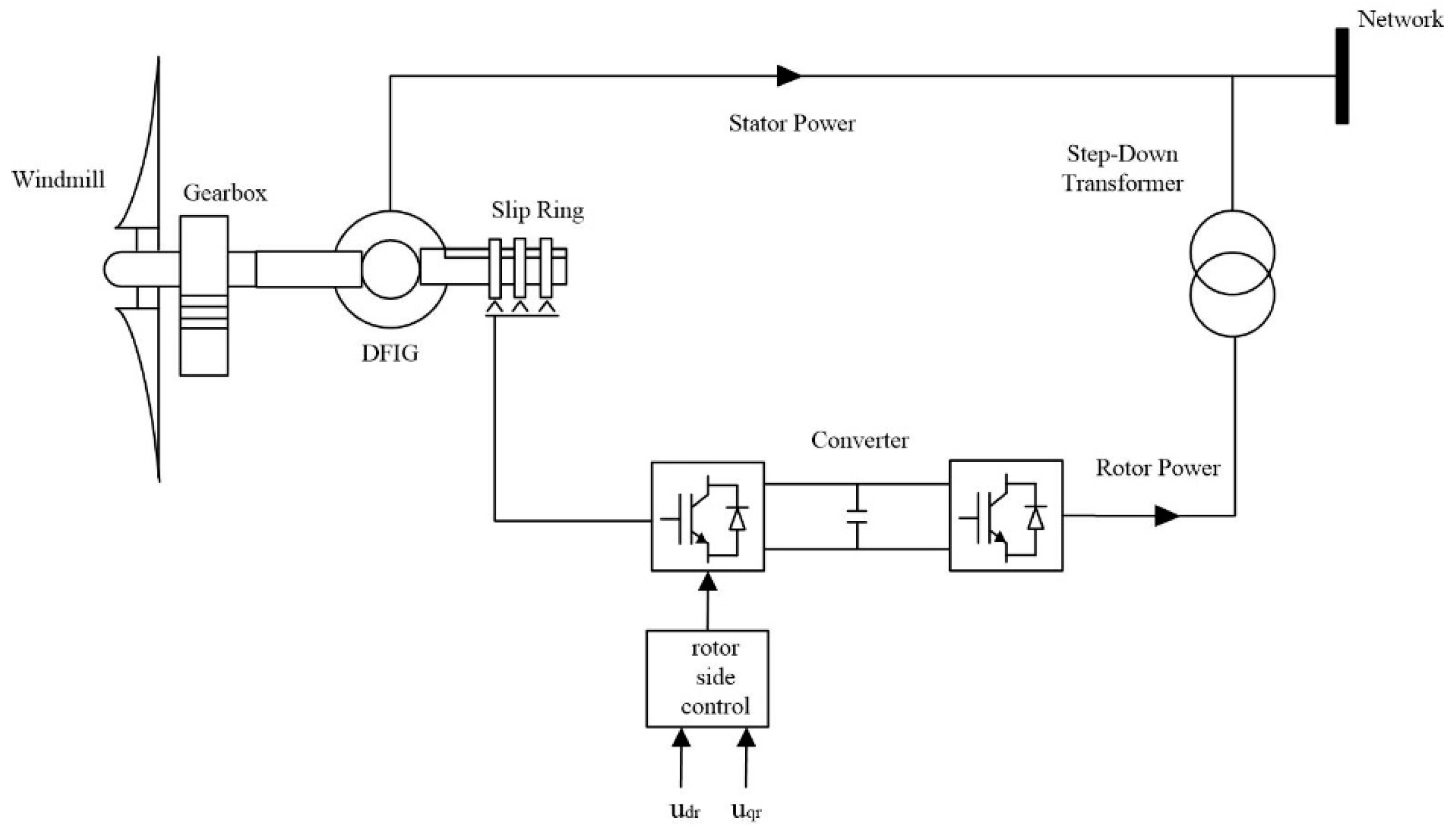
A wing wind power system with a doubly fed induction generator (DFIG) is sketched in Figure 1. Accordingly, the DFIG-based wind turbine system consists of a windmill, a gearbox, a doubly fed induction generator, a slip ring and a converter. Electrically, the DFIG stator is directly connected to a power grid and the rotor is connected to the power grid through a converter. The rotor side provides the excitation current with adjustable amplitude, phase and frequency. The intermediate converter is in the form of two back-to-back PWMs that can achieve four-quadrant operation. The DFIG has the advantages of variable speed and constant frequency such that maximum energy tracking and grid frequency synchronism under wind fluctuations can be achieved simultaneously. In principle, doubly fed means that the stator and rotor of the induction generator are connected to the power grid and thus both of them can create energy exchanges with the power grid. To realize doubly fed operations, PWM inverters are installed on the generator side, which make the rotor excitation flexible and fasten the power exchange [15].

2.1. Electromechanical Transient Modeling of DFIG

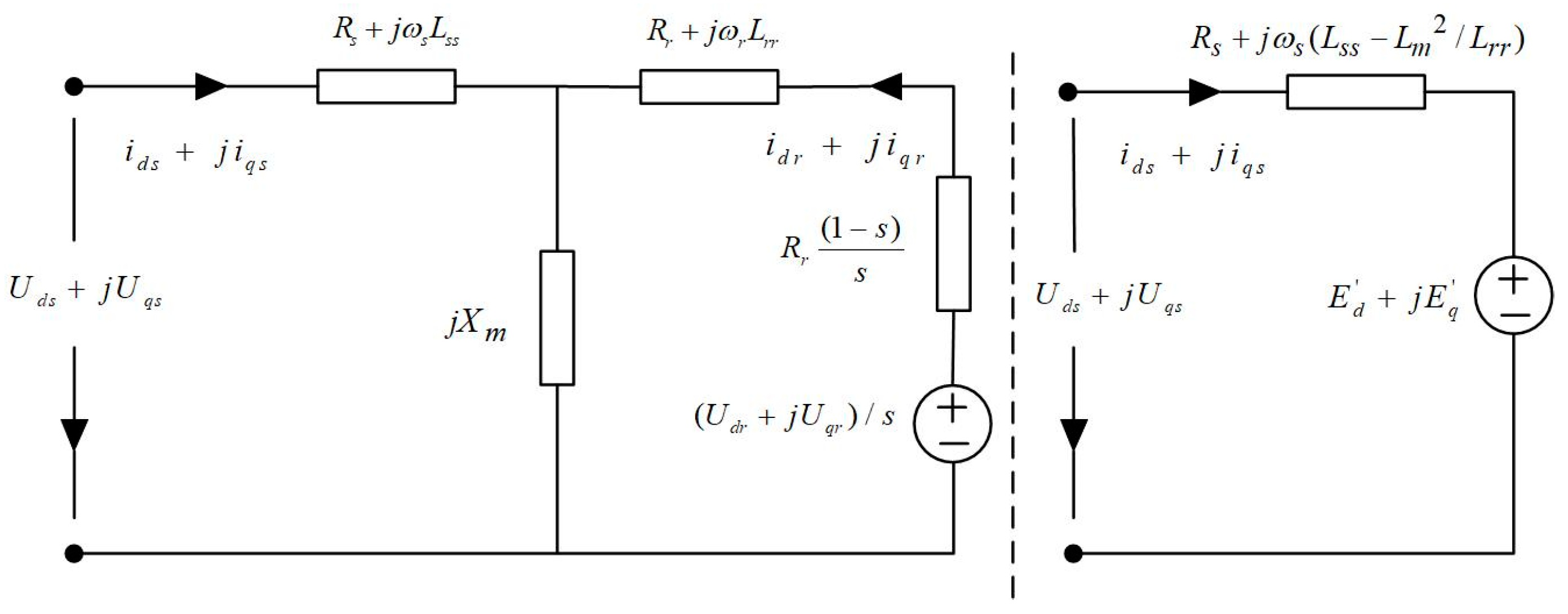
To model the electromechanical transient of the DFIG in the steady state, it is assumed that the steady state electromechanical transient is much slower than those of the electronic switching in devices such as the converters. Hence, it is reasonable to say that the switching dynamics of the electronic devices have died out where the electromechanical transience of the DFIG in the steady state is concerned. Together with DC capacitor voltage dynamics of the rotor being neglected, the steady state equivalent circuit of the DFIG is given in Figure 2.

As denoted in Figure 2, the subsequent notations are adopted throughout the paper. $s$ is the rotor slip rate; $L_{ss}$ and $L_{rr}$ are the stator and rotor self-inductances, respectively; $L_m$ and $X_m$ are the mutual inductance and reactance, respectively; $R_r$ and $R_s$ are the rotor and stator resistances, respectively; ${\omega }_s$ and ${\omega }_r$ are the synchronous angular velocity and rotor angular velocity, respectively; $U_{ds}(U_{dr})$ and $U_{qs}(U_{qr})$ are the $d-$ and $q-$ shaft stator (rotor) voltages, respectively; $E_d{}^{\prime }$ and $E_q{}^{\prime }$ are $d-$ and $q-$ shaft rotor voltages under the sub-transient, respectively; $i_{ds}(i_{dr})$ and $i_{qs}(i_{qr})$ are the $d-$ and $q-$ shaft stator (rotor) currents, respectively. In the above and what follows, the time variable t is dropped for simplicity.

The electromechanical transient of the DFIG in the steady state sense can be modeled as a third-order equation and its corresponding power equations:

$$\begin{array}{l}\left\{\begin{array}{l}2H\frac{d{\omega }_r}{dt}=T_m-T_e\\ \frac{d{E^{\prime }}_d}{dt}=-\frac{1}{T_{0^{\prime }}}[{E^{\prime }}_d-(L-L^{\prime })i_{qs}]+s{\omega }_s{E^{\prime }}_q-\frac{L_m}{L_{rr}}{u}_{qr}\\ \frac{d{E^{\prime }}_q}{dt}=-\frac{1}{T_{0^{\prime }}}[{E^{\prime }}_q+(L-L^{\prime })i_{ds}]-s{\omega }_s{E^{\prime }}_d+\frac{L_m}{L_{rr}}{u}_{dr}\end{array}\right.\\ \left\{\begin{array}{l}{P}_s=T_e={E^{\prime }}_d{i}_{ds}+{E^{\prime }}_q{i}_{qs}\\ Q_s={E^{\prime }}_d{i}_{ds}-{E^{\prime }}_d{i}_{qs}\end{array}\right.\end{array}$$

(1)

where $H$ is the inertia time constant of the wind turbine as a single mass point model. $T_m=F{\omega }_r$ and $T_e$ are the mechanical and electromagnetic torques on the generator rotor; $F$ is the force acting on the mechanical torque.

Due to the widespread use of power electronics technology, most of the current AC excitation power supplies of DFIGs use two back-to-back PWM converters. The dual PWM converters contain a net-side converter and a rotor-side converter. However, because of the small capacity of the DFIG exciter converter, the control capability of the whole wind turbine is weak. There are mainly field-oriented control (FOC), also called vector control (VC), and direct torque control (DTC) for the DFIG control system, currently. In this paper, the rotor-side converter of the wind turbines adopts the vector control strategy [16,17]. The rotor voltage control equation is:

$$\left\{\begin{array}{l}{u}_{dr}=R_r{i}_{dr}+\sigma L_{rr}\frac{d{i}_{dr}}{dt}-{\omega }_s\sigma L_{rr}{i}_{qr}\\ u_{qr}=R_r{i}_{qr}+\sigma L_{rr}\frac{d{i}_{qr}}{dt}+{\omega }_s(\frac{L_m}{L_{ss}}{\psi }_s+\sigma L_{rr}{i}_{dr})\end{array}\right.$$

(2)

where $\sigma =1-\frac{L_m^2}{L_{ss}{L}_{rr}}$.

It can be seen in (1) and (2) that if the rotor excitation power in the DFIG can be exploited as a voltage source, by controlling the rotor excitation voltages $u_{dr}$ and $u_{qr}$, while the sub-transient voltages ${E^{\prime }}_d$ and ${E^{\prime }}_q$ can be modified to achieve the DFIG power control objectives.

2.2. Linearization and State–Space Remodeling of DFIG

The equations in (1) and (2) together are nonlinear differential algebraic ones, whose analytical solution is not directly available. In other words, if Equations (1) and (2) are directly used for FF controller design, it will involve a large number of numerical integrations in controller parametrization, which will greatly reduce the operating speed of the controller. Therefore, the nonlinear differential equations need to be linearized in advance.

In (1), we rewrite ${\omega }_r=1-{\omega }_s$, selecting the operating point $({\omega }_{r0},i_{ds0},i_{qs0},E_{d0}{}^{\prime },E_{q0}{}^{\prime })$. Then, we select $\Delta {\omega }_r$, $\Delta {E^{\prime }}_d$, $\Delta {E^{\prime }}_q$ as state variables, $\Delta {\omega }_r$, $\Delta P^{\prime }$ and $\Delta Q^{\prime }$ as output measurements, $u_{dr}$ and $u_{qr}$ as input control actions. Due to the power electronic devices in the DFIG, switching harmonics are inevitable. Any distortion of the control waveform will be coupled to the stator side as harmonics [18]. Assuming the current harmonic of the stator $i_{ds}$ and $i_{qs}$ are viewed as disturbances. The linearized state–space model for the DFIG is

$$\left\{\begin{array}{l}\dot{x}(t)=Ax(t)+B_{1}p(t)+B_{2}u(t)\hfill \\ y(t)=Cx(t)+Du(t)\hfill \end{array}\right.$$

(3)

and

$$\left\{\begin{array}{l}A=\left[\begin{array}{ccc}-\frac{F}{2H}& -\frac{i_{ds0}}{2H}& -\frac{i_{qs0}}{2H}\\ -{E^{\prime }}_{q0}& -\frac{1}{T_{0^{\prime }}}& 1-{\omega }_{r0}\\ {E^{\prime }}_{d0}& {\omega }_{r0}-1& -\frac{1}{T_{0^{\prime }}}\end{array}\right]\in R^{3\times 3}, B_1=\left[\begin{array}{cc}0& 0\\ 0& \frac{L-L^{\prime }}{T_{0^{\prime }}}\\ -\frac{L-L^{\prime }}{T_{0^{\prime }}}& 0\end{array}\right]\in R^{3\times 2},\hfill \\ B_2=\left[\begin{array}{cc}0& 0\\ 0& -\frac{L_m}{L_{rr}}\\ \frac{L_m}{L_{rr}}& 0\end{array}\right]\in R^{3\times 2}, C=\left[\begin{array}{ccc}1& 0& 0\\ 0& i_{ds0}& i_{qs0}\\ 0& -i_{qs0}& i_{ds0}\end{array}\right]\in R^{3\times 3}, D=0.\hfill \end{array}\right.$$

2.3. Input Time Delay and Gain Disturbance in DFIG

The time delay in signal processing always exists in the state–space Equation (3). More specifically, feedback digital controllers require time to calculate and transmit, so the time delay is not simply avoidable. In this study, to improve the robustness of the DFIG against input delay, a memoryless state-feedback control (4) was applied to suppress current harmonics in the rotor current $p(t)$ of (3).

$$u(t)=(K+\Delta K(t))x(t-\tau ), t\in [0,\infty )$$

(4)

where $0<\tau <{\tau }_m$ is input time delay $K\in R^{2\times 3}$ is the static gain matrix to be designed, and $\Delta K\in R^{2\times 3}$ is gain disturbance caused during implementation but in the form of

$$\Delta K(t)=RU(t)TK$$

(5)

where $R\in R^{3\times 1}$ and $T\in R^{1\times 2}$ are the real constant, and $U(t)\in R$ is an unknown time varying continuous scalar function that satisfies $U^2(t)=U{(t)}^{T}U(t)\le I$.

Hence, the closed-loop system of the DFIG with the controller (4) is given by

$$\left\{\begin{array}{l}\dot{x}(t)=Ax(t)+B_{1}p(t)+B_2(K+\Delta K)x(t-\tau )\hfill \\ y(t)=Cx(t)+D(K+\Delta K)x(t-\tau )\hfill \end{array}\right.$$

(6)

In particular, when neglecting the gain disturbance $\Delta K$, the transfer function from $p(t)$ to $y(t)$ is denoted by $G_{py}(s,K)$ and given by

$$G_{py}(s,K)=(C+e^{-\tau s}DK){(s{I}_3-A-e^{-\tau s}{B}_{2}K)}^{-1}{B}_1\in C^{3\times 2}$$

(7)

where $I_3$ stands for the $3\times 3$ identity matrix.

2.4. FF Performance Specification for DFIGs

In the frequency domain, signals can be represented by several finite or infinite frequency trigonometric functions, which follow from the Fourier transform or generally the spectrum transform. For energy signals in power systems, the energy spectra are concentrated in some FF fashions. PWM is widely used in DFIGs, which includes harmonics in the air-gap magnetic field of the induction generator. One can impose some sinusoidal excitation voltage on the excitation circuit, and from the obtained spectra, the current harmonics are mainly in the frequency range of (250,550) Hz, as explained in [8]. In [9], it was also found that the DFIG frequency spectra of the output waveform are mainly concentrated around the integer multiplications of the switching frequency fs such as 2f_s, 3f_s, etc. With respect to the (2,4) kHz converter switching frequency, external current harmonics to the DFIG are mainly around (2,8) kHz. In [19,20], specifications of grid harmonics are summarized among (50,150) Hz. Therefore, if FF features of switching and disturbances are not taken into account in $H_{\infty }$ control, no practical optimal performance in the DFIG can be obtained.

$${\Omega }_d=\{\omega \in R|(\omega -{\omega }_1)(\omega -{\omega }_2)\le 0\}=[{\omega }_1,{\omega }_2]$$

(8)

where ${\omega }_2>0$ and ${\omega }_1>0$ are the upper and lower bounds for frequencies in harmonic interference and disturbance, respectively. Now we are ready to introduce the finite frequency (FF) performance for our later use.

Definition 1.

Considering the system (6), the FF $H_{\infty }$ performance index of $G_{py}(s,K)$ is

$$\Vert G_{py}(j\omega ,K){\Vert }_{\infty }^{{\Omega }_d}:=\underset{\omega \in {\Omega }_d}{\sup }\overline{\sigma }[G_{py}(j\omega ,K)]>0$$

where $\overline{\sigma }(\cdot )$ denotes the maximum singular value of $(\cdot )$, and $G_{py}(j\omega ,K)$ is given in (7).

2.5. Problem Formulation

The control problem for the DFIG in Figure 1 is: fix the controller $K$ in Equation (5) such that the corresponding augmented-state system (7) is asymptotically stabilized when $\Delta K=0$, and with respect to a given scalar $\gamma >0$, the $H_{\infty }$ performance in the FF interval ${\Omega }_d$ satisfies

$$\Vert G_{py}(j\omega ,K){\Vert }_{\infty }^{{\Omega }_d}<\gamma$$

To address the formulated problem, the following lemmas will be exploited.

Lemma 1

([21]). For the transfer function $G_{py}(s,K)$ in (8), if there exists a matrix $\Pi ={\Pi }^T$ such that

$$\left[\begin{array}{cc}{G}_{py}^H(j\omega )& I\end{array}\right]\Pi \left[\begin{array}{c}{G}_{py}(j\omega ,K)\\ I\end{array}\right]<0, \forall \omega \in [{\omega }_1,{\omega }_2]$$

if and only if there exist matrices $P=P^T$,  $X=X^T$,  $Q=Q^T$and  $Z=Z^T$satisfying

$$\begin{array}{l}{\left[\begin{array}{ccc}A& B_{2}K& B_1\\ I& 0& 0\end{array}\right]}^T(\Phi \otimes P+\Psi \otimes Q+{\Psi }_0\otimes {\tau }_{m}Z)\left[\begin{array}{ccc}A& B_{2}K& B_1\\ I& 0& 0\end{array}\right]n\\ +{\left[\begin{array}{ccc}C& DK& 0\\ 0& 0& I\end{array}\right]}^T\Pi \left[\begin{array}{ccc}C& DK& 0\\ 0& 0& I\end{array}\right]+\left[\begin{array}{ccc}X-{\tau }_m^{-1}Z& {\tau }_m^{-1}Z& 0\\ {\tau }_m^{-1}Z& -X-{\tau }_m^{-1}Z& 0\\ 0& 0& 0\end{array}\right]<0\end{array}$$

(9)

where

$$\Psi =\left[\begin{array}{cc}-1& j{\omega }_c\\ -j{\omega }_c& -{\omega }_1{\omega }_2\end{array}\right],{\Psi }_0=\left[\begin{array}{cc}1& 0\\ 0& 0\end{array}\right], \Phi =\left[\begin{array}{cc}0& 1\\ 1& 0\end{array}\right], \Pi =\left[\begin{array}{cc}1& 0\\ 0& -{\gamma }^{2}I\end{array}\right]$$

In the above,  ${\omega }_2\ge {\omega }_1>0$and  ${\omega }_c=({\omega }_1+{\omega }_2)/2$are used.

Lemma 2

(Projection Lemma [22]). For matrices $\Psi ={\Psi }^T$, $K$ and $M$, there exists a matrix $X$ satisfying $\Psi +\mathrm{He}(KXM)<0$, if and only if $K^{\perp }\Psi K^{\perp }{}^T<0$ and ${(M^T)}^{\perp }\Psi {(M^T)}^{\perp }{}^T<0$.

Lemma 3

(Jensen Inequality [23]). For any matrix $P=P^T>0\in R^n$, a scalar $\lambda >0$, a vector function $\omega :[0,\lambda ]\to R_n$ such that the following integrals are well-defined, then

$${\displaystyle {\int }_0^{\lambda }{\omega }^T(s)P\omega (s)ds}\ge {({\displaystyle {\int }_0^{\lambda }\omega (s)ds})}^{T}P({\displaystyle {\int }_0^{\lambda }\omega (s)ds})$$

Lemma 4

([23]). Given matrices $Q=Q^T$, $R$ $T$ of appropriate dimensions, we have

$$Q+RU(t)T+T^T{U}^T(t)R^T<0, \forall t\ge 0$$

(10)

for any $U(t)$ satisfying $U^T(t)U(t)<I$, if and only if there exists a scalar $\mu >0$ such that

$$\left[\begin{array}{ccc}Q& \mu R& T^T\\ *& -\mu I& 0\\ *& *& -\mu I\end{array}\right]<0$$

(11)

Several remarks about Lemmas 1 to 4:

• Lemma 1 follows from the generalized Kalman–Yakubovich–Popov (GKYP) lemma, which is a frequency domain criterion that guarantees the existence of Lyapunovv–Krasovskii functionals for stability analysis in nonlinear systems via strict positive realness in terms of transfer function [24,25]. In other words, the GKYP lemma provides us with time/frequency domain stability conditions. However, the LMI inequality of Lemma 1 must be interpreted in the time–domain fashion but related to some FF factors of the transfer function.
• The assumption that $(A,B_1,C)$ is a minimal state–space realization of $G_{py}(s,K)$ is needed for generalizing the KYP lemma rigorously [26]. Thus, the pair $(A,B_1)$ is controllable, and the pair $(A,C)$ is observable.
• Lemmas 2–4 can be interpreted both in the time and frequency domain ways. Confined to our discussion, they are used only in the time–domain fashion.
• The inequality (10) of Lemma 4 is a time–domain inequality. The equivalent inequality (11) should be interpreted also in the time–domain way if we retrieve the proof arguments between (10) and (11). The point plays a key role in combining the results in Lemmas 1 and 4.

3. FF $H_{\infty }$ Controller Design of DFIG

In this section, a criterion of the FF H_∞ controller is presented for DFIGs with input time delay, which guarantees asymptotic stability and the desired H_∞ performance of the closed-loop DFIG system in (6). There will be four theorems to explain the controller design procedures, where the stability conditions in LMI are given in Section 3.1, LMIs under the harmonic interference attenuation condition are formulated in Section 3.2, and the H_∞ controller design and parametrization are provided in Section 3.3.

3.1. Stability Analysis

Theorem 1.

For any delay $0<\tau <{\tau }_m$, the closed-loop DFIG system (6) with $\Delta K=0$ is asymptotically stable, if there exist a scalar $\alpha >0$ and matrices $P_1=P_1{}^T>0$, $R_1=R_1{}^T>0$,$S_1=S_1{}^T>0$ and $J$ such that the inequality ${\Theta }_1<0$ holds. Here, ${\Theta }_1={\Theta }_1^T$

$${\Theta }_1=\left[\begin{array}{ccc}{\tau }_m{S}_1-\alpha \mathrm{He}(J)& P_1-\alpha J+\alpha J^{T}A& \alpha J^T{B}_{2}K\\ *& R_1-{\tau }_m^{-1}{S}_1+\alpha \mathrm{He}(A^{T}J)& \alpha J^T{B}_{2}K+{\tau }_m^{-1}{S}_1\\ *& *& -R_1-{\tau }_m^{-1}{S}_1\end{array}\right]<0$$

(12)

The proof of Theorem 1 is given inAppendix A.1.

3.2. FF-Domain $H_{\infty }$ Performance Analysis

Theorem 2.

Let the FF interval ${\Omega }_d$ be defined in (8) and the delay $0<\tau <{\tau }_m$ and a scalar $\gamma >0$ be given. Then, the closed-loop DFIG system (6) with $\Delta K=0$ satisfies the FF $H_{\infty }$ performance inequality $\Vert G_{py}(s,K){\Vert }_{\infty }^{{\Omega }_d}<\gamma$, if there exist matrices $P_2=P_2{}^T>0$, $Q_2=Q_2{}^T>0$, $X=X^T>0$, $Z=Z^T>0$ and $J$ such that the inequality ${\Theta }_2<0$ holds. Here, ${\Theta }_2={\Theta }_2^T$ is given by

$${\Theta }_2=\left[\begin{array}{ccccc}-Q_2+{\tau }_{m}Z& P_2+j{\omega }_c{Q}_2-J& 0& 0& 0\\ *& -{\omega }_1{\omega }_2{Q}_2+\mathrm{He}(A^{T}J)+X-{\tau }_m^{-1}Z& J^T{B}_{2}K+{\tau }_m^{-1}Z& J^T{B}_1& C^T\\ *& *& -X-{\tau }_m^{-1}Z& 0& K^T{D}^T\\ *& *& *& -{\gamma }^{2}I& 0\\ *& *& *& *& -I\end{array}\right]$$

(13)

The proof of Theorem 1 is given inAppendix A.2.

3.3. FF Controller Parametrization

It must be noticed that in Theorems 1 and 2, the gain disturbance $\Delta K$ is not considered. To enhance the stability robustness of the closed-loop system (6) against gain disturbance $\Delta K\ne 0$ by means of the practical controller $K+\Delta K$, the results of Theorems 1 and 2 must be modified. The following theorem can be obtained by using Lemma 4.

Theorem 3.

For any time delay $0<\tau <{\tau }_m$, there exists a controller (4) with gain disturbance $\Delta K=RU(t)TK$ constrained by (5) such that the closed-loop system (6) is asymptotically stabilized and satisfies the FF $H_{\infty }$ performance, if there exist matrices $P_1=P_1{}^T>0$, $R_1=R_1{}^T>0$, $S_1=S_1{}^T>0$, $P_2=P_2{}^T>0$ $Q_2=Q_2{}^T>0$, $X=X^T>0$, $Z=Z^T>0$ and a general matrix $J$, the following LMIs holds true.

$${\Theta }_3={\Theta }_3^T=:\left[\begin{array}{ccccc}{\varphi }_{11}& {\varphi }_{12}& {\varphi }_{13}& {\varphi }_{14}& 0\\ *& {\varphi }_{22}& {\varphi }_{23}& {\varphi }_{24}& 0\\ *& *& {\varphi }_{33}& 0& {\varphi }_{35}\\ *& *& *& -\mu I& 0\\ *& *& *& *& -\mu I\end{array}\right]<0$$

(14)

$$\mathit{where}\left\{\begin{array}{ll}{\varphi }_{11}={\tau }_m{S}_1-\alpha \mathrm{He}(J),\hfill & {\varphi }_{12}=P_1-\alpha J+\alpha J^{T}A\hfill \\ {\varphi }_{13}=\alpha J^T{B}_{2}K,\hfill & {\varphi }_{14}=\mu \alpha J^T{B}_{2}R\hfill \\ {\varphi }_{22}=R_1-{\tau }_m^{-1}{S}_1+\alpha \mathrm{He}(A^{T}J),\hfill & {\varphi }_{23}=\alpha J^T{B}_{2}K+{\tau }_m^{-1}{S}_1\hfill \\ {\varphi }_{24}={\varphi }_{14}, {\varphi }_{33}=-R_1-{\tau }_m^{-1}{S}_1,\hfill & {\varphi }_{35}=K^T{T}^T\hfill \end{array}\right.$$

$${\Theta }_4={\Theta }_4^T=:\left[\begin{array}{ccccccc}{\Psi }_{11}& {\Psi }_{12}& 0& 0& 0& 0& 0\\ *& {\Psi }_{22}& {\Psi }_{23}& J^T{B}_1& C^T& \mu J^T{B}_{2}R& 0\\ *& *& {\Psi }_{33}& 0& K^T{D}^T& 0& K^T{T}^T\\ *& *& *& -{\gamma }^{2}I& 0& 0& 0\\ *& *& *& *& -I& \mu DR& 0\\ *& *& *& *& *& -\mu I& 0\\ *& *& *& *& *& *& -\mu I\end{array}\right]<0$$

(15)

$$\mathit{where}\left\{\begin{array}{l}{\Psi }_{11}=-Q_2+{\tau }_{m}Z, {\Psi }_{12}=P_2+j{\omega }_c{Q}_2-J\hfill \\ {\Psi }_{22}=-{\omega }_1{\omega }_2{Q}_2+\mathrm{He}(A^{T}J)+X-{\tau }_m^{-1}Z\hfill \\ {\Psi }_{23}=J^T{B}_{2}K+{\tau }_m^{-1}Z, {\Psi }_{33}=-X-{\tau }_m^{-1}Z\hfill \end{array}\right.$$

The proof of Theorem 1 is given inAppendix A.3.

Since the LMIs in (14) and (15) involve the product terms of $K$ and $J$, they cannot be handled directly by means of the LMI numerical toolkit. To decouple such product terms, let us define

$$W_1=\mathrm{diag}[J^{-T},J^{-T},J^{-T}], W_2=\mathrm{diag}[J^{-T},J^{-T},J^{-T},I,I]$$

Then, we pre- and post-multiply Equations (22) and (23) with $W_1$, $W_1^T$ and $W_2$, $W_2^T$, respectively. Additionally, we introduce the notations as follows.

$$\left\{\begin{array}{l}{\overline{P}}_1=J^{-T}{P}_1{J}^{-1}, {\overline{R}}_1=J^{-T}{R}_1{J}^{-1}, {\overline{S}}_1=J^{-T}{S}_1{J}^{-1}\hfill \\ {\overline{P}}_2=J^{-T}{P}_2{J}^{-1}, {\overline{Q}}_2=J^{-T}{Q}_2{J}^{-1}, \overline{Z}=J^{-T}Z{J}^{-1}\hfill \\ \overline{X}=J^{-T}X{J}^{-1}, V=K{J}^{-1}, \overline{J}=J^{-1}\hfill \end{array}\right.$$

Using these notations, we can claim the following theorem.

Theorem 4.

For any time delay $0<\tau <{\tau }_m$, there exists a controller (4) with gain disturbance $\Delta K=RU(t)TK$ constrained by (5) such that the closed-loop system (6) is asymptotically stabilized and satisfies the FF $H_{\infty }$ performance, if there exist matrices $\overline{P_1}={\overline{P}}_1{}^T>0$, ${\overline{R}}_1={\overline{R_1}}^T>0$, $\overline{S_1}={\overline{S_1}}^T>0$, ${\overline{P}}_2={\overline{P_2}}^T>0$, $\overline{Q_2}={\overline{Q_2}}^T>0$, $\overline{X}={\overline{X}}^T>0$, $\overline{Z}={\overline{Z}}^T>0$ and a general matrix $\overline{J}$, $V$ such that the following LMIs holds true.

$${\overline{\Theta }}_3={\overline{\Theta }}_3^T=:\left[\begin{array}{ccccc}{\overline{\varphi }}_{11}& {\overline{\varphi }}_{12}& {\overline{\varphi }}_{13}& {\overline{\varphi }}_{14}& 0\\ *& {\overline{\varphi }}_{22}& {\overline{\varphi }}_{23}& {\overline{\varphi }}_{24}& 0\\ *& *& {\overline{\varphi }}_{33}& 0& {\overline{\varphi }}_{35}\\ *& *& *& -\mu I& 0\\ *& *& *& *& -\mu I\end{array}\right]<0$$

(16)

$$\mathit{where}\left\{\begin{array}{l}{\overline{\varphi }}_{11}={\tau }_m{\overline{S}}_1-\alpha \mathrm{He}(\overline{J}), {\overline{\varphi }}_{12}={\overline{P}}_1-\alpha {\overline{J}}^T+\alpha A\overline{J}\hfill \\ {\overline{\varphi }}_{13}=\alpha B_{2}V, {\overline{\varphi }}_{14}=\mu \alpha B_{2}R\hfill \\ {\overline{\varphi }}_{22}={\overline{R}}_1-{\tau }_m^{-1}{\overline{S}}_1+\alpha \mathrm{He}(A\overline{J}), {\overline{\varphi }}_{23}=\alpha B_{2}V+{\tau }_m^{-1}{\overline{S}}_1, {\overline{\varphi }}_{24}=\mu \alpha B_{2}R\hfill \\ {\overline{\varphi }}_{33}=-{\overline{R}}_1-{\tau }_m^{-1}{\overline{S}}_1, {\overline{\varphi }}_{35}=V^T{T}^T\hfill \end{array}\right.$$

$${\overline{\Theta }}_4={\overline{\Theta }}_4^T=:\left[\begin{array}{ccccccc}{\overline{\Psi }}_{11}& {\overline{\Psi }}_{12}& 0& 0& 0& 0& 0\\ *& {\overline{\Psi }}_{22}& {\overline{\Psi }}_{23}& B_1& {\overline{J}}^T{C}^T& \mu B_{2}R& 0\\ *& *& {\overline{\Psi }}_{33}& 0& V^T{D}^T& 0& V^T{T}^T\\ *& *& *& -{\gamma }^{2}I& 0& 0& 0\\ *& *& *& *& -I& \mu DR& 0\\ *& *& *& *& *& -\mu I& 0\\ *& *& *& *& *& *& -\mu I\end{array}\right]<0$$

(17)

$$\mathit{where}\left\{\begin{array}{l}{\overline{\Psi }}_{11}=-{\overline{Q}}_2+{\tau }_m\overline{Z}, {\overline{\Psi }}_{12}={\overline{P}}_2+j{\omega }_c{\overline{Q}}_2-{\overline{J}}^T\hfill \\ {\overline{\Psi }}_{22}=-{\omega }_1{\omega }_2{\overline{Q}}_2+\mathrm{He}(A\overline{J})+\overline{X}-{\tau }_m^{-1}\overline{Z}, {\overline{\Psi }}_{23}=B_{2}V+{\tau }_m^{-1}\overline{Z}\hfill \\ {\overline{\Psi }}_{33}=-\overline{X}-{\tau }_m^{-1}\overline{Z}\hfill \end{array}\right..$$

Moreover, the control gain $K$ can be given by $K=V{\overline{J}}^{-1}$.

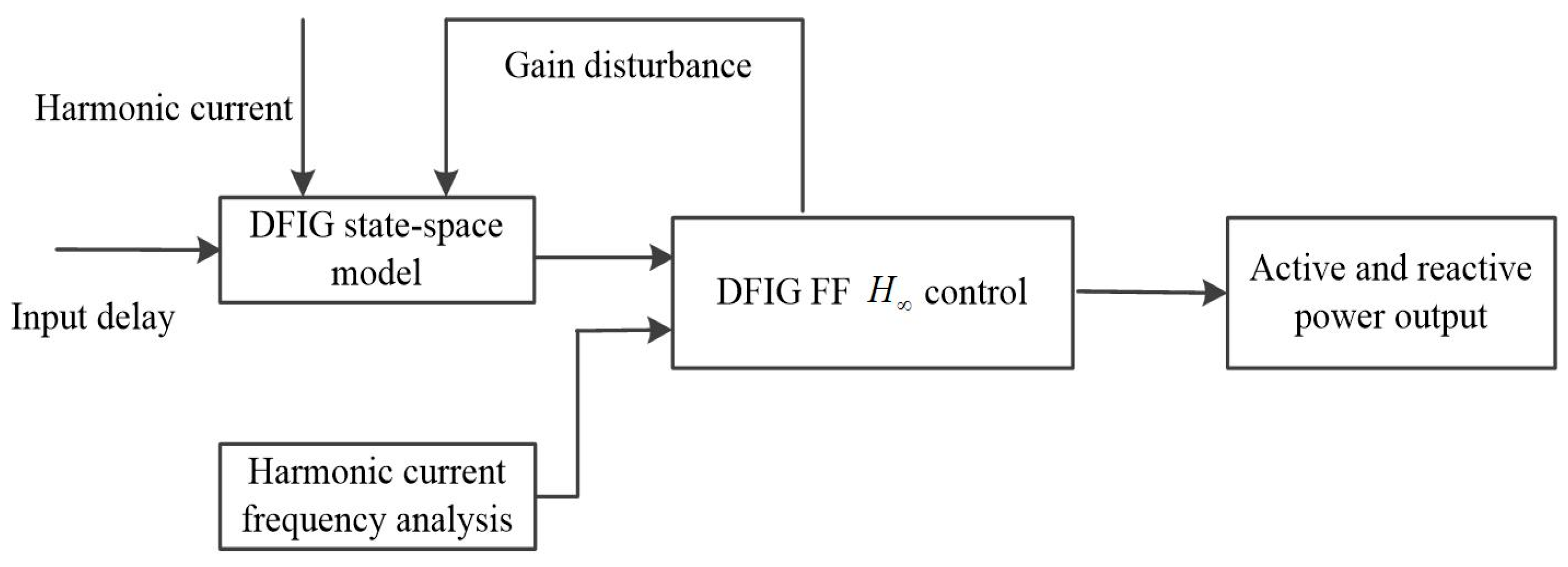
The FF $H_{\infty }$ control for the DFIG flow chart is shown in Figure 3. control for DFIG flow chart.

4. Numerical Simulations

In this section, we illustrate effectiveness of the suggested FF $H_{\infty }$ control strategies.

4.1. Descriptions about DFIG and Control Design

The modeling parameters of the 5 MW wind turbine DFIGs are: $H=6\sec$,$L_m=0.4 \mathrm{p}.\mathrm{u}.$, $L_{rr}=0.55 \mathrm{p}.\mathrm{u}.$, $L_{ss}=0.17 \mathrm{p}.\mathrm{u}.$, $R_r=0.5 \mathrm{p}.\mathrm{u}.$, $i_{ds0}=1.8 \mathrm{p}.\mathrm{u}.$,$i_{qs0}=1.7 \mathrm{p}.\mathrm{u}.$, $E_{ds0}=2.8 \mathrm{p}.\mathrm{u}.$, $E_{qs0}=2.7 \mathrm{p}.\mathrm{u}.$, ${\omega }_{r0}=3.14 \mathrm{p}.\mathrm{u}.$. The linearized DFIG state–space equation matrices in the sense of (9) is given by

$$\begin{array}{l}A=\left[ \begin{array}{ccc}-2& -0.15& -0.14\\ -2.7& -1& -2.14\\ 2.8& 2.14& -1\end{array}\right], B_1=\left[\begin{array}{cc}0& 0\\ 0& 0.3\\ -0.3& 0\end{array}\right], \\ B_2=\left[\begin{array}{cc}0& 0\\ 0& -0.7\\ 0.7& 0\end{array}\right], C=\left[\begin{array}{ccc}1& 0& 0\\ 0& 1.8& 1.7\\ 0& -1.7& 1.8\end{array}\right], D=0\end{array}$$

The finite frequency domain interval of the current harmonic interference is first estimated as $2 \mathrm{kHz}<{\omega }_d<8 \mathrm{kHz}$. We assume that ${\tau }_m=100 \mathrm{ms}$. Given $\alpha =1$, $\gamma =1$, $\mu =0.3$, $R=1$, $U=1$, $T=0.005$, we solve the corresponding LMIs (22) and (23) in Theorem 4. The FF controller $K$ is fixed as

$$K=\left[\begin{array}{ccc}-1.859& -0.570& -2.250\\ -1.368& 1.986& -1.392\end{array}\right]$$

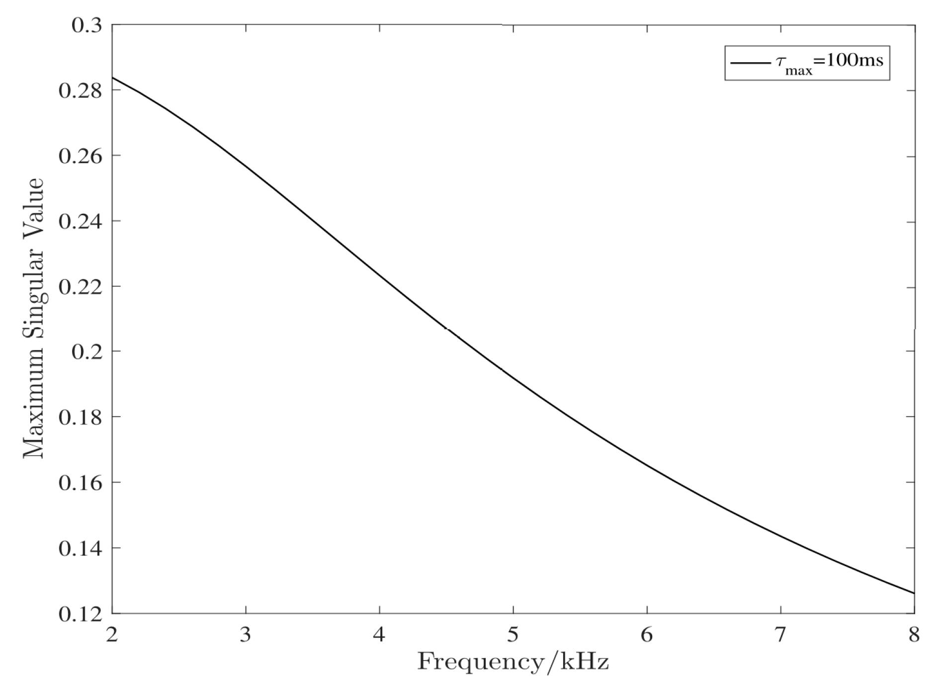
The frequency characteristics for the maximum singular value of $G_{py}(s,K)$ is plotted in Figure 4. We see that the max value of $\Vert G_{py}(j\omega ,K)\Vert$ is 0.283, which is strictly less than $\gamma =1$.

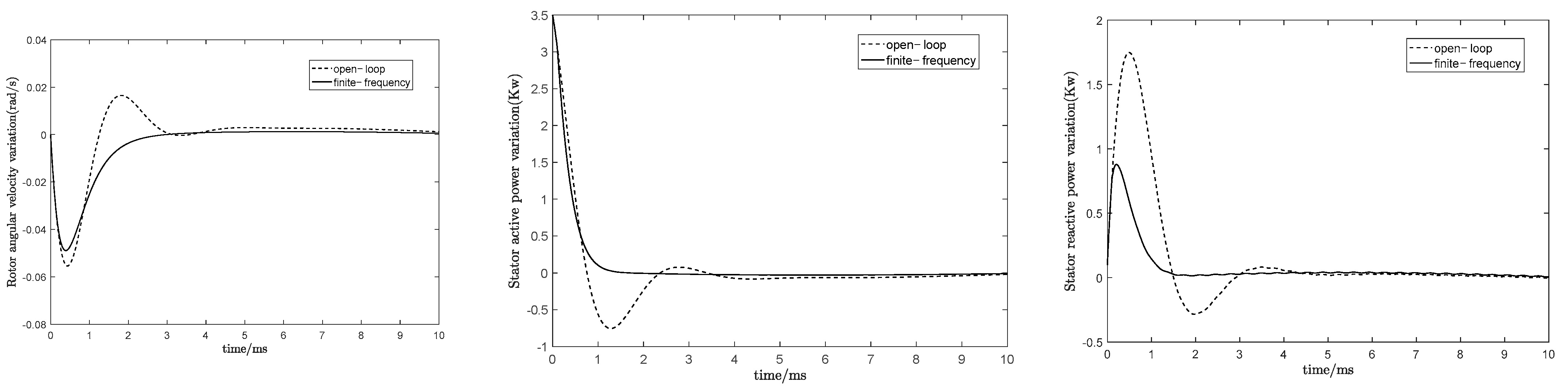
Now we consider the cases subject to current harmonic interference. More specifically, the harmonic interference is in the form of $p(t)=0.1\sin (2\pi ft)$($f$ = 3 kHz). The DFIG rotor angular velocity, the stator active and reactive power responses in the open-loop system (by dotted lines) and those in the closed-loop system (by solid lines) are plotted in Figure 5.

In Figure 5, we see that the oscillation amplitude of the closed-loop responses under the FF $H_{\infty }$ control is smaller, and the response convergence is faster than that of the open-loop responses. It shows that the FF $H_{\infty }$ controller reduces the transient time period while it stabilizes the closed-loop system.

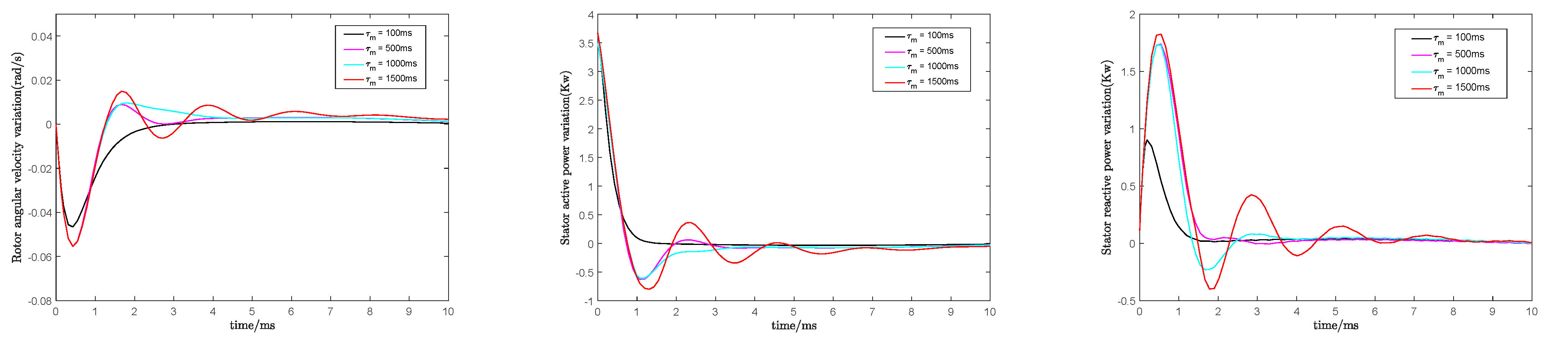
4.2. Cases under Various Time Delays

To reveal how the time delay upper bound ${\tau }_m$ is related to the FF $H_{\infty }$ performance, we made a comparison computation when ${\tau }_m\in \{100,500,1000,1500\}\mathrm{ms},$ respectively. The $H_{\infty }$ controller parametrization under different ${\tau }_m$s are collected in

Table 1. The Gain Matrix $K$ under different ${\tau }_m$s.

Delay/ms	Feedback Gain Matrix $\mathit{K}$	Feasibility
100	$K=\left[\begin{array}{ccc}-1.859& -0.570& -2.250\\ -1.368& 1.986& -1.392\end{array}\right]$	$\surd$
500	$K=\left[\begin{array}{ccc}-0.199& -0.075& -0.280\\ -0.808& 0.586& -0.265\end{array}\right]$	$\surd$
1000	$K=\left[\begin{array}{ccc}-0.243& -0.3& 0.330\\ -0.741& -0.199& -0.272\end{array}\right]$	$\surd$
1500	$K=\left[\begin{array}{ccc}-0.619& -0.542& 0.212\\ -0.702& -0.217& -0.503\end{array}\right]$	$\surd$

. The response curves of the DFIG rotor angular velocity, stator active and reactive powers are plotted in Figure 6, where w.r.t. is the abbreviation for with respect to. By Figure 6, one can see that the larger the delay upper bound is, the worse (or the bigger) the resulting $H_{\infty }$ performance index is.

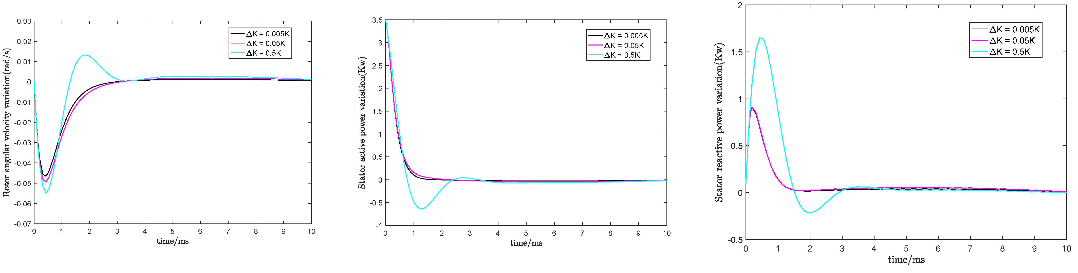
4.3. Cases under Various Gain Disturbances

To illustrate how the gain perturbation $\Delta K$ affects the control performance, we selected $R=1$, $U=1$, and the weighting factor $T\in \{0.005,0.05,0.5\}$, respectively. Substituting $R$, $U$, $T$ into the Equation (5), we obtained the corresponding $\Delta K\in \{0.005K,0.05K,0.5K\}$. Then, we compared the control performances under different $\Delta K$. The $H_{\infty }$ controller gain matrix $K$ are listed in

Table 2. The Gain Matrix $K$ under different $\Delta K$.

$\mathbf{\Delta }\mathit{K}$	Feedback Gain Matrix $\mathit{K}$	Feasibility
0.005 $K$	$K=\left[\begin{array}{ccc}-1.859& -0.57& -2.25\\ -1.368& 1.986& -1.392\end{array}\right]$	$\surd$
0.05 $K$	$K=\left[\begin{array}{ccc}-1.816& -0.533& -2.197\\ 1.312& 1.949& -1.342\end{array}\right]$	$\surd$
0.5 $K$	$K=\left[\begin{array}{ccc}-0.152& -0.047& -0.145\\ -0.025& 0.12& -0.071\end{array}\right]$	$\surd$

. The response curves of DFIG rotor angular velocity, stator active and reactive powers are plotted in Figure 7. By Figure 7, it is easy to deduce that as the control gain perturbation $\Delta K$ grows, the corresponding $H_{\infty }$ performance deteriorates obviously.

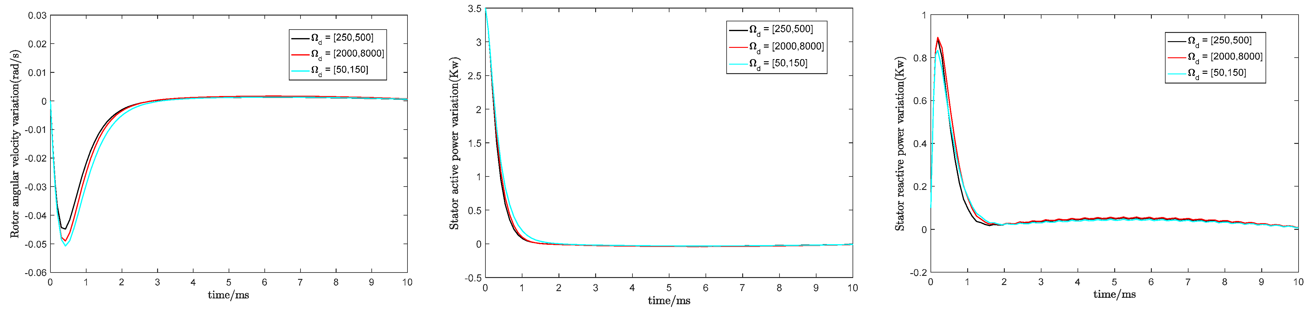
4.4. Cases for Various Finite Frequency Domain Intervals

To reveal the $H_{\infty }$ control performance under different current harmonic frequency interval ${\Omega }_d$s, we evaluate several when ${\Omega }_d\in \{[50,150]\mathrm{Hz},[250,550]\mathrm{Hz},[2000,8000]\mathrm{Hz}\}$. The corresponding $H_{\infty }$ controller parametrizations for different ${\Omega }_d$ are listed in

Table 3. The Gain Matrix $K$ under different ${\Omega }_d$s.

${\mathbf{\Omega }}_{\mathit{d}}$/Hz	Feedback Gain Matrix $\mathit{K}$	Feasibility
$50<{\Omega }_d<150$	$K=\left[\begin{array}{ccc}-2.27& -0.884& -2.137\\ -1.657& 1.688& -1.676\end{array}\right]$	$\surd$
$250<{\Omega }_d<550$	$K=\left[\begin{array}{ccc}-1.908& -0.575& -2.5714\\ -1.569& 2.523& -1.508\end{array}\right]$	$\surd$
$2000<{\Omega }_d<8000$	$K=\left[\begin{array}{ccc}-1.859& -0.570& -2.25\\ -1.368& 1.986& -1.392\end{array}\right]$	$\surd$

The response curves of DFIG rotor angular velocity, stator active and reactive powers are plotted in Figure 8. From Figure 8, we can see that the $H_{\infty }$ control can well suppress the current harmonics interference in all three cases. This verifies the effectiveness and robustness of the suggested controller.

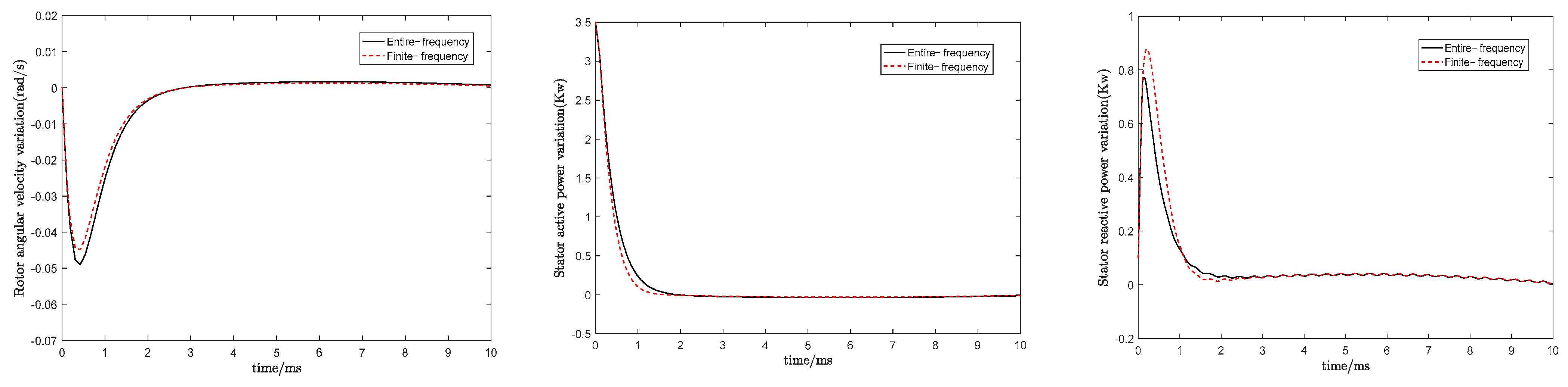
4.5. Cases Comparison under FF and EF $H_{\infty }$ Control

Finally, we compared the H_∞ control performances in the finite frequency (FF) sense with those in the entire-frequency (EF) sense. In Figure 9, the dotted lines and the solid lines, respectively, represent the response curves of the DFIG power systems under the FF H_∞ and EF H_∞ control. Clearly, the response curves related to the FF H_∞ controller are smoother, while the overshoots are less, and thus the control performance under the FF H_∞ control is significantly enhanced.

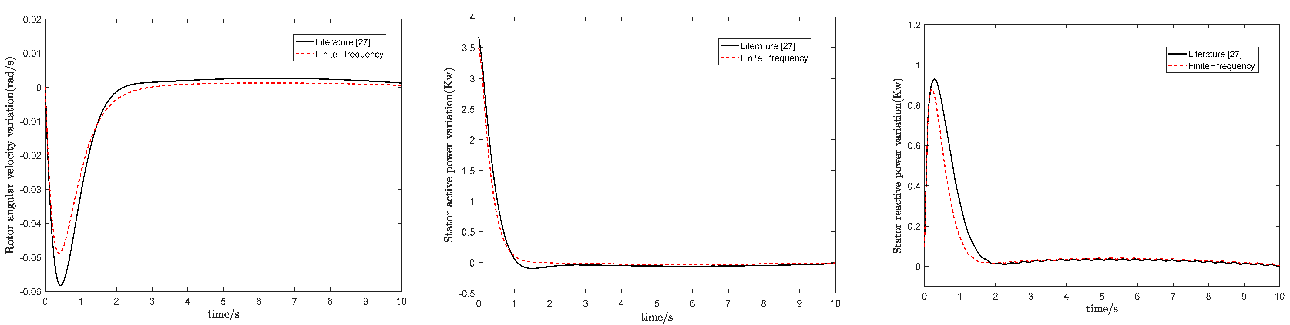
4.6. Cases Comparison under FF and Other $H_{\infty }$ Control Methods

Finally, for comparison, the FF $H_{\infty }$ control method in this paper and the general $H_{\infty }$ control method in the literature [27] are applied in this example where parameters are chosen as ${\tau }_m=100\mathrm{ms}$, $\Delta K=0.005K$. It is evident from Figure 10 that the control performance under the FF $H_{\infty }$ control proposed in this paper is significantly improved compared to the ones in the literature [27].

5. Discussions

In this paper, a state-feedback control scheme is proposed, which caters for the FF control problem for the DFIG system with the time delay, current harmonics and gain disturbances. This method is of great significance in improving the robustness of wind power systems.

The third order DFIG turbine model adopts a one-mass drive and ignores the stator transient, so some flux components are not responsible for the turbine’s decaying and oscillating modes. This model is more suitable for real DFIG systems. Then the state–space model for DFIGs was obtained using Taylor’s formula.

In large power systems, electricity may oscillate in a short period of time due to time delays, which reflects badly on turbines, power equipment and the power grid. The harmonic interferences and gain disturbances in the power system can reduce the power quality, leading to lower generation efficiency and higher generation costs for wind farms. It is necessary to study the time delay control of large-scale wind power systems under current harmonic disturbances and gain disturbances.

For the DFIG state–space model with input delay under current harmonics and gain disturbances model, an FF H_∞ state-feedback controller was designed from the frequency domain perspective, which makes the DFIG stable and robust against harmonic interferences and gain disturbances. Using the generalized KYP lemma and Lyapunov theory, the FF performance was evaluated using linear matrix inequalities, and the state feedback parametrization was addressed based on this. This method improves the utilization rate of wind energy and is a feasible and effective control method in wind power systems.

In summary, the method proposed in this paper is technically and economically advantageous in terms of power generation performance, system simplification and cost- effectiveness. A new control technology and system structure were applied to analyze power systems and improve the power quality.

Potential applications of the method are as follows.

• At present, the control technology of wind power technology is relatively mature. The FF H_∞ control design method in this paper provides a new frequency domain design idea for the suppression of disturbances in various uncertain cases of wind power systems, which can improve the quality of power systems.
• With the development of distributed wind power systems in wind farms, the distributed wind turbines based on FF H_∞ control for doubly fed induction generators with input delay and the gain disturbance control strategy proposed in this paper could be used in wind farms, which can realize the efficient use of wind energy.

6. Conclusions

In view of DFIG wind turbine systems, the FF H_∞ control method was proposed for systems with input delay under controller gain disturbance and current harmonic interference. By employing the GKYP lemma and Lyapunov theory, the FF H_∞ control problem can be transformed into an LMI feasible solution problem. Interesting results are claimed as in Theorems 1–4. The main contributions and novelty of the proposed methods in this paper can be summarized by the following aspects:

• A control strategy in terms of the frequency band is formulated for the DFIG by taking time delay and gain disturbance into account, and it has not been fully considered in previous studies on the control of the DFIG.
• Based on the GKYP lemma and the Lyapunov theory, sufficient conditions are formulated for the DFIG with input delay to satisfy the desired specification in the frequency band. Then, the frequency design problem of DFIGs is transformed into a time domain LMI problem, which significantly facilitated our solution process.
• A sufficient condition is presented to search for the optimal FF controller for the DFIG. Furthermore, the output of active and reactive power was stable, which improved the stability and reliability of the system. This design method provided new ideas for the development and application of DFIG control in the future.

As possible extensions of the FF LMI technique in DFIG engineering, the following control problems are significant and interesting, which will be addressed in our subsequent studies.

• The model for DFIGs in this paper is 3-dimensional. Next, higher order systems with higher dimensional DFIG systems can be considered [28,29].
• Sliding mode control: $u(t)=f(t,x(t),x(t-\tau ))$ over a sliding surface $S(t,x(t),x(t-\tau ))$ can be applied to achieve finite-time convergence.
• Apply the results for networked DFIGs via multi-agent consensus [30,31,32].