Fully Distributed Water Balance Modelling in Large Agricultural Areas—The Pinios River Basin (Greece) Case Study

Abstract

Robust assessments of variations in freshwater availability are essential for current and future water resource management in the Pinios River Basin (PRB), which is one of the most productive basins of Greece in terms of agriculture. To support sustainable water resources management in the PRB, we set up and calibrated the mGROWA hydrological model at a high spatial (100 m) and temporal (daily) resolution for the period 1971–2000, with particular attention given to deriving crop-specific irrigation requirements. We developed and implemented a comprehensive methodological framework to overcome data scarcity constraints in the PRB, thus enabling the derivation of high-resolution spatially continuous estimates of many input variables required for the mGROWA model. We generated estimates of spatiotemporal variations in the water balance components actual evapotranspiration, irrigation requirements, total runoff, and groundwater recharge for the PRB. In addition, through the calculation of indices, such as the potential irrigation to groundwater recharge ratio (PIQR), we demonstrate a way to identify potential unsustainable water use in irrigated agriculture. The established mGROWA model can be used both as a hydrological reference model providing continuous decision support for water resources management, focusing on irrigation water use, and a basis for climate impact studies for the PRB.

1. Introduction

The Mediterranean region is one of the world’s climate change hot spots [1]. Numerous studies concerning the Mediterranean region have found that droughts and water scarcity associated with climate change constitutes a major threat to current and future water supplies (e.g., [2,3]). In Greece, climate change has already contributed to decreasing precipitation since the 1990s [4,5,6], while rising temperatures have simultaneously led to increasing reference evapotranspiration [7]. Because of these climatic trends, dramatic changes in runoff volume relative to historical conditions should be expected by the middle of the upcoming century [8,9]. In this context, a robust assessment of the uncertain changes in freshwater availability is essential for current and future water resource management in Greece [10].

An essential prerequisite for the effective management of water resources is the reliable characterisation of historical time series of hydrological processes, comprising non-stationarity [11]. Water balance models can provide the broad data basis necessary for such studies. Hydrological modelling in semiarid areas, and especially in the Mediterranean region, is marked by high complexity [12] and strong non-linearity associated with the significant seasonal fluctuations in precipitation and temperature. For this reason, the overall objective of this study is to establish a fully distributed high-resolution water balance model for the Pinios River Basin (PRB) in central Greece using the mGROWA model [13] and analyse the results.

The mGROWA model was developed to provide high-resolution, ready for use estimates for the water balance components of large catchments or administrative areas, originally for the federal states Lower Saxony and North Rhine-Westphalia in Germany [13,14]. The federal states require estimates of renewable water resources and allocate water rights based on the mGROWA model outputs of the spatiotemporal distributions of groundwater recharge. Because the simulated soil moisture pattern is an important pre-condition for irrigation modelling, mGROWA was further developed through the integration of an irrigation module to study the impact of irrigation practices on the regional water balance in the Hamburg Metropolitan Region (Germany) [15]. Due to the flexible parameterisation options of the model, mGROWA has been adapted and applied to Mediterranean conditions, e.g., for areas in France, Italy, and Turkey [16,17,18]. As the methodology implemented in mGROWA allows the modelling of the impacts of climate change according to the rating system described by Refsgaard et al. [11], the model has also been applied in climate impact studies in Germany [13] and the Mediterranean [16,17].

The PRB presents a hydrological regime within a complex geomorphological environment and high seasonal and interannual variability of water balance components [19], while also being used for intensive irrigated agriculture. A sub optimal organisation of irrigation systems [20,21] and unsustainable water resources management practices [22] have deteriorated the already disturbed water balance and accelerated the degradation of water resources in previous decades. This study additionally aims to: (a) supplement and add to the existing diverse assessment studies and data provided by model implementations in the whole PRB, its sub-catchments, groundwater bodies, and other administrative sub-areas, e.g., as described in [23,24,25,26,27,28]; and (b) facilitate the implementation of sustainable water resources management practices.

In particular, the spatiotemporal distribution of groundwater recharge in the PRB is not adequately addressed by the aforementioned studies. One of the key objectives in our study is therefore to reduce the uncertainty concerning the characterisation of site conditions that control groundwater recharge and to quantify its potential range over time and space. Considering the above, as well as the necessity to develop effective water management plans within the context of the Water Framework Directive (2000/60/EC), this study aims to:

• describe the implementation of the fully distributed water balance model mGROWA (Section 3) in the PRB (Section 2),
• identify the implementation difficulties of such a hydrological model in a highly complex yet data-scarce Mediterranean basin (Section 4),
• provide insights into the hydrological processes of the PRB, (Section 5),
• provide qualitative and quantitative water balance assessments of the PRB (Section 5) and their evaluation (Section 6),
• demonstrate the potential usability of this model as a water resources management tool in Greece (Section 6 & Section 7), and
• provide a robust basis for further studies of climate change impacts on water resources in the PRB (Section 7).

We modelled the hydrologic period 1971–2000 due to limited climate data availability for more recent time periods and because this period is used as the historical control period of the EURO-CORDEX RCM ensemble [29]. We have set up the mGROWA model in the PRB on a 100 m grid and it is simulating water balance in daily resolution.

2. Materials and Methods

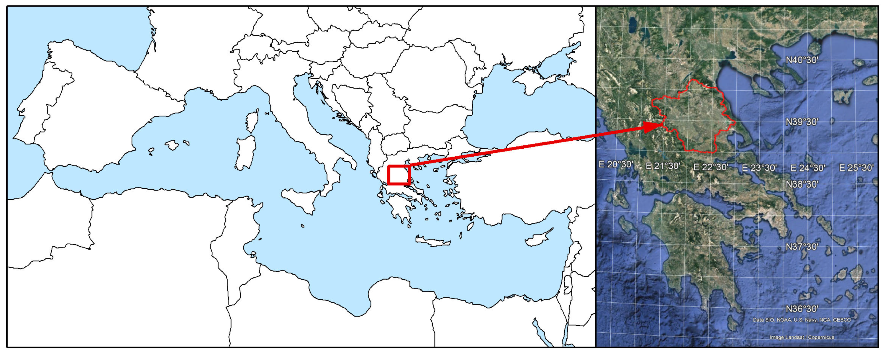
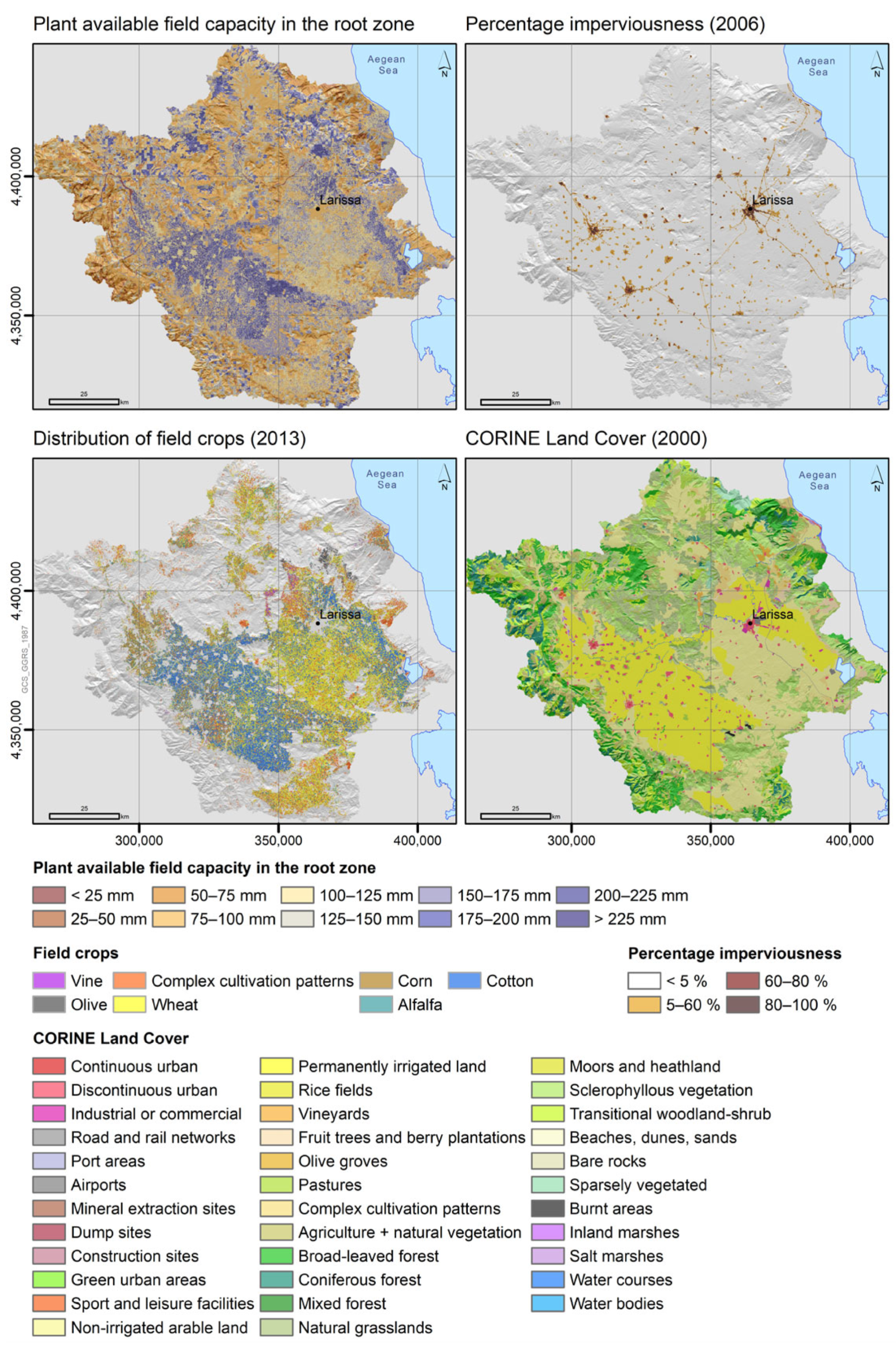
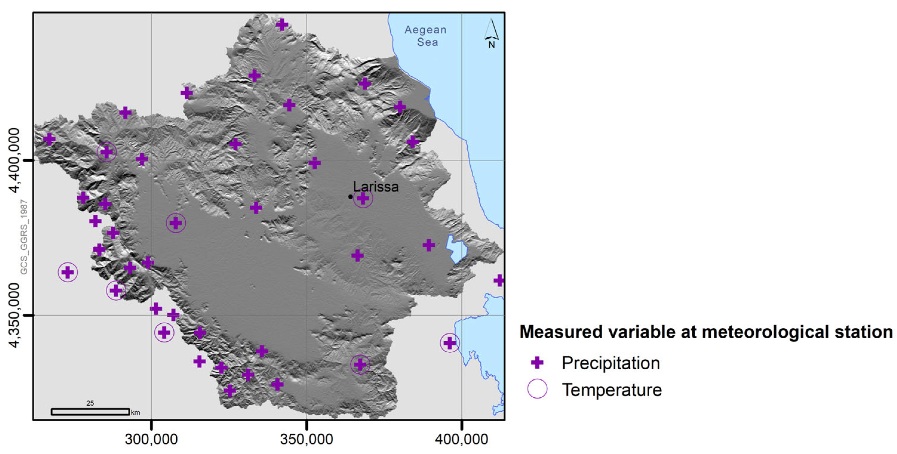
Located in central Greece, the PRB covers an area of about 11,000 km², and is the 2nd largest fully developed basin in Greece (Figure 1). The PRB covers about 85% of the Thessaly Water District [30], which according to the 2021 census, had a population of about 687,500. The PRB constitutes a highly diversified geologic, hydrological, and geomorphological environment and is surrounded by a rugged relief reaching altitudes of over 2000 m. 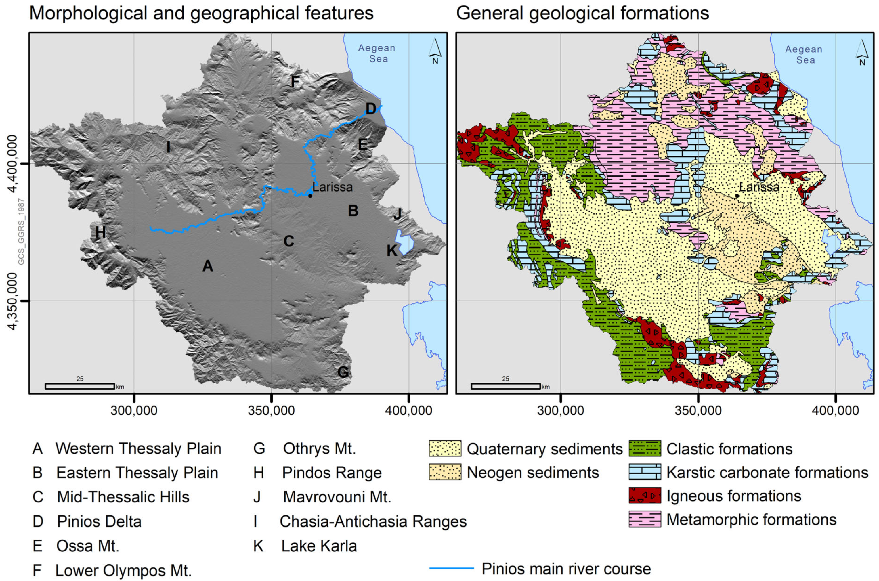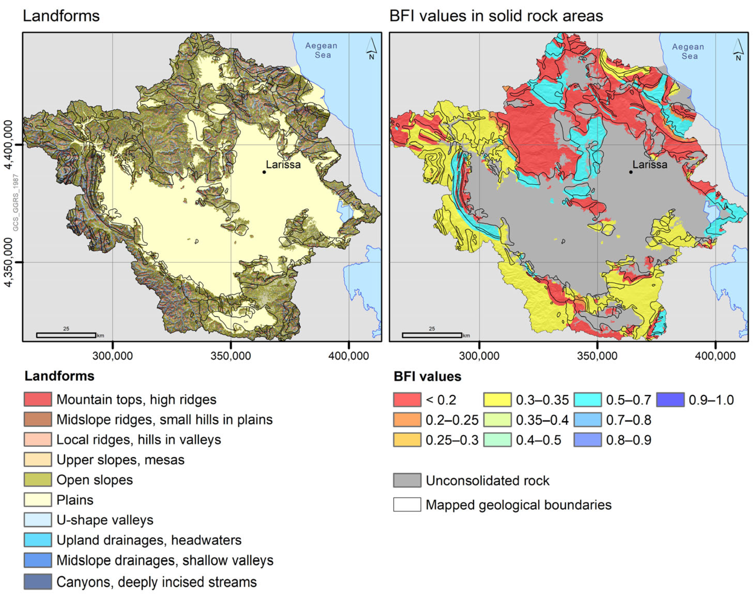Figure 2 shows the location of major geomorphological and geographical features in the PRB.

The PRB is subdivided into two major sub-basins, namely the Eastern and Western Thessaly basins (Figure 2A,B), which exhibit significantly different geologic and hydroclimatic characteristics. A low-lying hill area (Figure 2C) comprising of karstified carbonate rocks [31,32] divides the two sub-basins. Along the riverine zone of Pinios River and in its delta (Figure 2D), alluvial and recent deposits are prevalent, followed by Neogene formations (conglomerates, sandstones, clays, marls, and terrestrial-lacustrine deposits). Aquifers of medium to high water abstraction potential have developed within these formations. In the mountain ranges (Figure 2E–I) around the two plains, Mesozoic and Paleozoic solid rock formations (mainly crystalline limestones, marbles, gneisses, and schists) dominate [32]. Due to the high degree of karstification in some parts of the basin, the corresponding aquifers display high water abstraction potential and are strongly influencing the groundwater budget of the PRB through springs and lateral crossflows recharging the alluvial aquifers of the plain [26].

The PRB is characterised by continental and Mediterranean climate conditions with dry and warm to hot summers, and precipitation concentrated in the winter months. According to Beck et al. [33], the Köppen–Geiger climate classification indicates BSk (arid, steppe, cold) in the Eastern Thessaly plain, Csa (temperate, dry and hot summer) in the Western Thessaly plain and both Csb and Dsb (temperate, dry and warm summer; cold, dry and warm summer) in the mountain ranges. The basin-averaged annual precipitation for the period 1981–2000 was estimated as 700 mm [34].

The PRB is one of the most intensively cultivated and productive agricultural areas in Greece, with agriculture corresponding to about 45% of the total basin area. Annual crops such as cotton, wheat, and corn are most common in the plains, while orchards (mainly apples, cherries, and vine) are located at the foothills of the mountain ranges. Hills and mountain ranges are forested with sclerophyllous and coniferous vegetation or covered by Mediterranean scrubland.

Almost 94% of the total water abstraction in the PRB is allocated to irrigation [35]. Since the 1980s, the increasing water demand for irrigation requirements accompanied by irrational water management practices have resulted in significant overexploitation of groundwater resources. Currently, more than 65% of the total water consumption is served by groundwater, emphasising the importance of groundwater for the sustainability of the area. According to the most recent regional water management plan [35], nine of the 27 groundwater bodies recognised in the PRB have been designated as of bad quantity [31]. They are subject to recurring quantitative groundwater stress [36]. In addition, the reservoirs in the region of the former Lake Karla (Figure 2K) play an important role in supplying the Eastern Thessaly plain with irrigation water [37]. The former Lake Karla was fully drained by 1962. Its reconstruction started in 1999 and was finalised in 2018. Nowadays the re-constructed reservoir is designed to store water originating from the southern mountains, as well as redirected winter runoff from the Pinios River, provided by a water diversion and a network of channels and ditches [38,39].

3. mGROWA Model Description

The water balance model mGROWA [13] has been developed for assessing the water balance over large areas (river basins, states, etc.) under present and possible future climate conditions. mGROWA constitutes a new generation of the water balance model GROWA [40], which has been used in numerous water balance studies in Germany and the Mediterranean region since the beginning of the 2000s, as presented in the section of Introduction. For a detailed description of the GROWA/mGROWA modelling approach, the reader is referred to the corresponding literature. Here, we briefly introduce the basic concepts and modules of most importance for modelling the PRB.

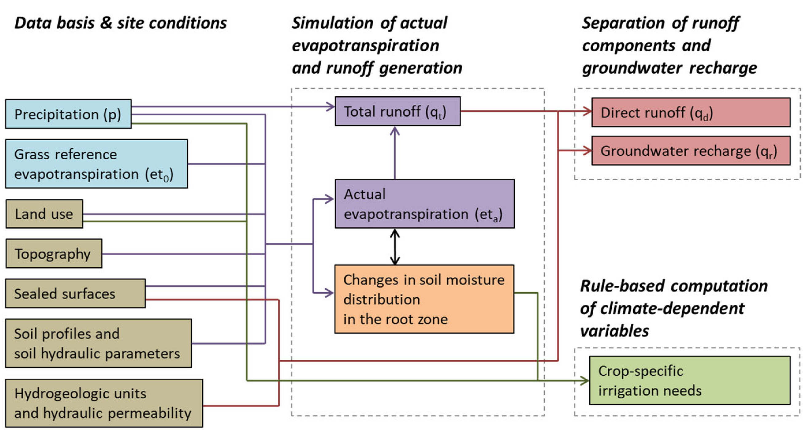
The distributed grid-based mGROWA model uses a two-step calculation process. Firstly, the water balance and runoff formation at the ground surface layer, which includes the root zone of the soil, is simulated using a physically based approach. Building on that, an empirical approach is used to provide a mass-separation of the total formed runoff into in-situ groundwater recharge and other diffuse water fluxes occurring near-surface in the unsaturated zone, accumulated as direct runoff. Sets of distributed gridded parameters are required, which characterise the in-situ processes in a generalised way. Thus, the spatial accuracy of mGROWA simulations is highly dependent on the quality and resolution of these input parameters.

3.1. Simulation of the Total Water Balance

The underlying formula for the first part of the simulation constitutes the generic water balance equation, with its climatic, runoff and storage terms given as:

$$\frac{ds}{dt}=p+irr-e{t}_a-q_t$$

(1)

where p represents the precipitation, irr the irrigation, et_a the actual evapotranspiration, q_t the total runoff, s the amount of water stored in a grid cell, and t the time. All values represent a vertical water height in mm. For grid cells with vegetation or bare soils, s corresponds to the soil moisture (θ), whereas for artificially sealed surfaces (e.g., buildings, paved roads, etc.), s represents the water stored on these impervious surfaces. For grid cells partially covered by impervious surfaces (PI refers to the percentage imperviousness), the simulation is executed in the two independent modes soil with vegetation (SWV-mode) and sealed ground surface (SGS-mode), and afterwards merged.

In the mGROWA model, special attention has been paid to the calculation of actual evapotranspiration and the associated storage functions:

$$e{t}_a=e{t}_0\times k_c\times f\left(SI,SA\right)\times f\left(s\right)$$

(2)

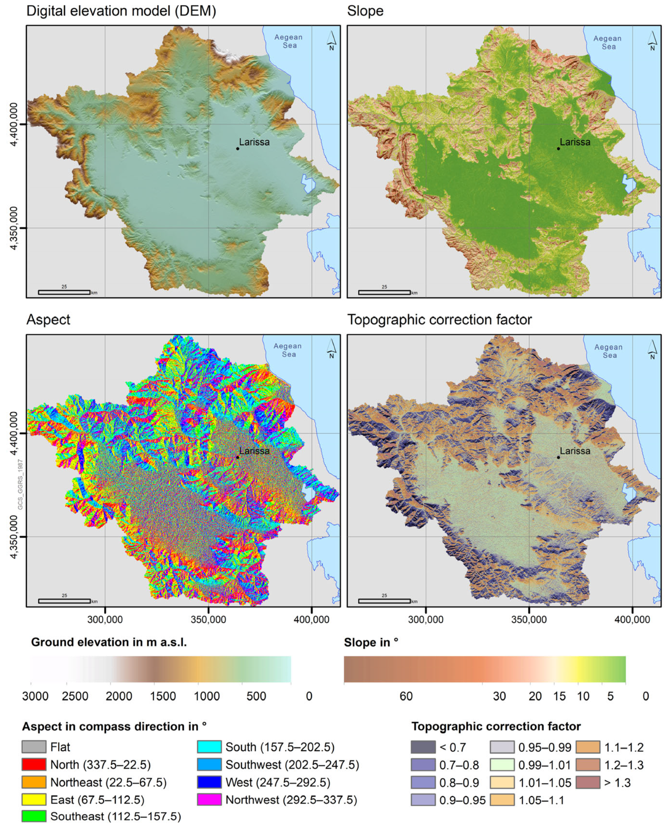
The grass reference evapotranspiration et₀ is commonly determined based on the Penman–Monteith equation, as given in [41] or alternative equations depending on the available climate data (see Section 4.4). k_c is a land use and vegetation (or crop) specific evapotranspiration factor (also known as crop coefficient). f(SI,SA) represents a topography function that accounts for slope (SI) and aspect (SA) (details in [40]). f(s) is a storage function which considers the water available for evapotranspiration. In the SWV-mode, f(s) is solved by a multi-layer soil module (MLSM). In the PRB model domain, we simulated the vertical soil moisture dynamics using five soil layers of 3 dm thickness each. In each layer, the total soil water storage is characterised by the plant available field capacity θ_a (details in Section 4.2) and the rooting depth RD. The functional dependence of evapotranspiration on soil moisture is given by the Disse-function [42]:

$$f\left(\theta \right)=\frac{1-e^{-r\times \frac{\theta -{\theta }_{pwp}}{{\theta }_a}}}{1+e^{-r\times \frac{\theta -{\theta }_{pwp}}{{\theta }_a}}-2\times e^{-r}}$$

(3)

where e is the Euler number, r is a vegetation-specific factor, θ_pwp the soil moisture at the permanent wilting point, θ_a the plant available soil moisture of the soil at field capacity (i.e., the difference between the soil moisture at field capacity θ_fc and θ_pwp), and θ the actual soil moisture. The Disse-function provides values in the range of 0 to 1. When the soil moisture decreases to the permanent wilting point, actual evapotranspiration becomes 0. When the soil water storage reaches the field capacity, actual evapotranspiration is not diminished, i.e., the level of potential evapotranspiration is reached.

Because of the intensive irrigation of most field crops in the PRB, irrigation-triggered evaporation fluxes must be incorporated into basin-wide water balance assessments. For this purpose, mGROWA provides an irrigation module (IM) that indirectly includes this flux by estimating the spatial variation of the irrigation requirements of field crops on a daily basis and linking irrigation water inputs to the MLSM. Irrigation of field crops commonly follows specific rules which are intended to ensure economically justified expenses and soil water content values at a plant-physiological level that promise optimal yields. The IM utilises the simulated soil moisture status of the MLSM and crop-specific sets of rules, which reflect the common irrigation management practices of farmers, in order to determine irrigation sequences and water quantities. The following rules and constraints are implemented (details in [15]), and the corresponding parameters are introduced in Section 4.2:

• irrigation-relevant root zone,
• soil water content that initiates irrigation,
• soil water content at which irrigation stops,
• maximum irrigation level per day,
• period of the year with potential irrigation application,
• minimum precipitation level per day for which no irrigation is applied,
• total water budget available for irrigation in a predefined period (according to water usage rights allocated to a farmer or field plot).

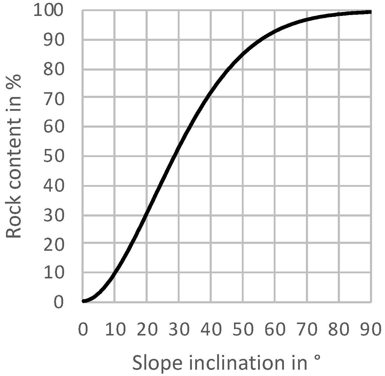
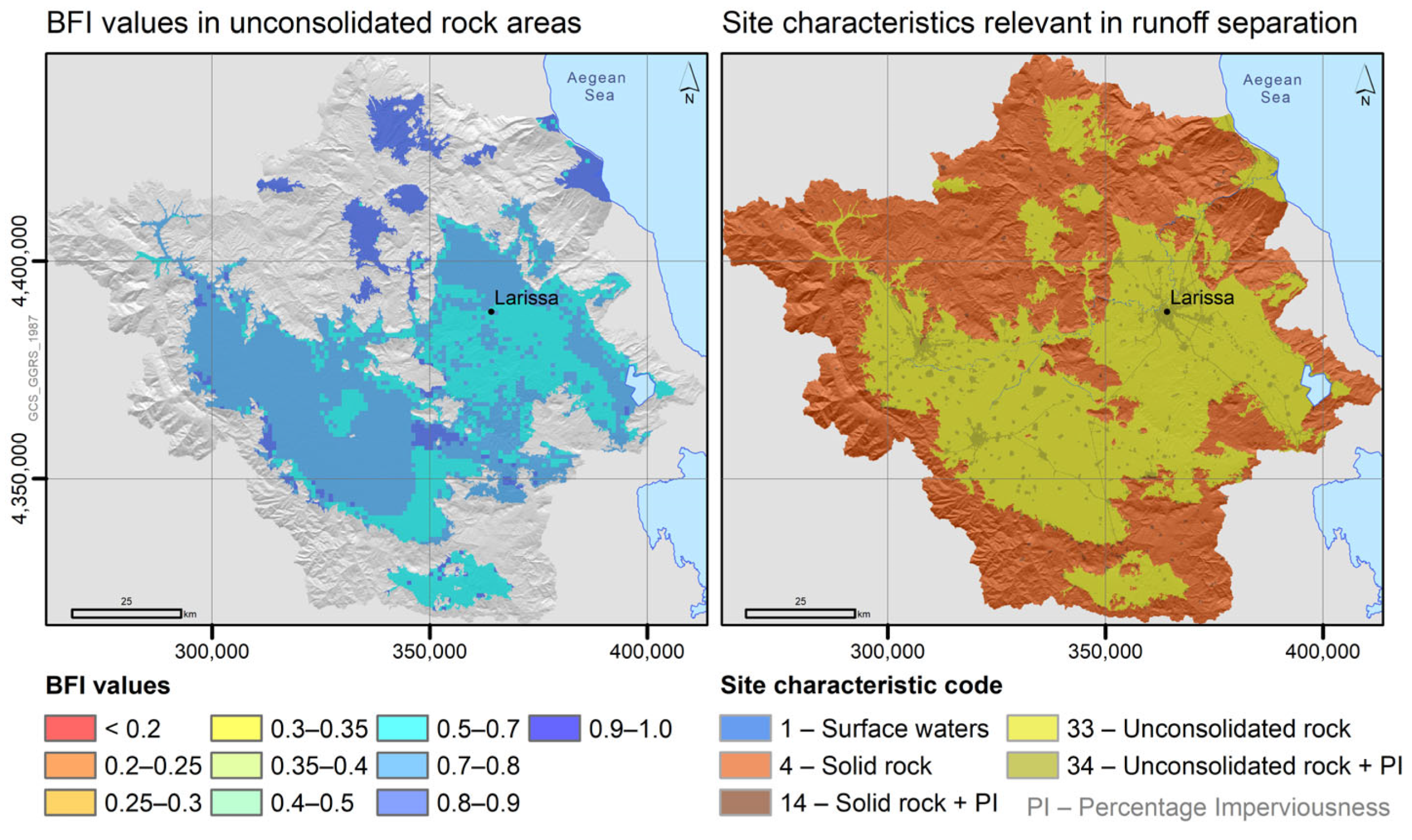
According to Equation (1), total runoff is calculated as the surplus water that cannot be stored in the root zone of soil against gravity or on an impervious surface due to its limited water storage capacity. The daily surplus water is then separated into groundwater recharge and direct runoff (incorporating quick runoff components) within the subsequent empirical part of the simulation.

3.2. Runoff Separation

For the overall water balance simulation, runoff separation is also split into two modes depending on the presence of artificially sealed surfaces (SGS-mode). For impervious shares of grid cells, the surplus water that cannot be stored on the surface is balanced as quick urban direct runoff and attributed to the direct runoff (q_d). The runoff characteristics of grid cells (or shares) without ground surface sealing (SWV-mode) are assigned using empirically derived distributed BFI values (base flow indices) which describe groundwater recharge (q_r) as a constant portion of total runoff:

$$q_r=q_t\times BFI=q_t-q_d$$

(4)

The BFI values depend on natural site conditions (details in Section 4.3) and can be regarded as constant in the long-term. Because groundwater recharge equals base flow in the long-term (under the assumption of hydrological stationarity), BFIs derived from discharge hydrographs can be regionalised and correlated with spatially distributed site conditions (e.g., soil or geologic properties) and resulting distributed BFI values can thus be utilised to estimate area-differentiated in-situ groundwater recharge [40,43]. In the mGROWA model, q_d is the residual of such calculations (see Equation (4)) and comprises the fast and moderate-fast runoff components, such as overland flow and interflow, however, without separating them into these individual components.

4. Data Processing and Model Parameterisation

4.1. Data Collection and Sources

The quantitative and spatial accuracy of the water balance components simulated using mGROWA crucially depend on the quality and spatial resolution of the input data used in the model. Special attention had to be paid to the parameterisation of the PRB model domain because of a lack of high-resolution datasets. The input datasets used in the context of the mGROWA implementation in the PRB are summarised in

Table 1. Data input requirements of the mGROWA model accompanied by a description of the corresponding dataset used for implementation in the PRB.

Input Requirements	Dataset, Source, and Description
Topography	The digital elevation data from the 90 m SRTM (Version 4) dataset [44] was used.
Surface sealing	Spatial data on the degree of surface sealing (percentage imperviousness PI) from buildings, paved roads, etc., was acquired from the Copernicus Land Monitoring Service (https://land.copernicus.eu/, accessed on 20 January 2023). We used the high resolution layer Imperviousness Density (20 m pixel size) representing the year 2015.
Land cover	Spatial data on common vegetation and land use types originate from the CORINE Land Cover (CLC) inventory and was acquired from the Copernicus Land Monitoring Service (https://land.copernicus.eu/, accessed on 20 January 2023). We used the map from 1990 (time consistency 1986–1998) at 100 m resolution.
Crop type and distribution	The spatial distribution of crops in the PRB on the farm level in the year 2013 was collected from the Hellenic Payment and Control Agency for Guidance and Guarantee Commu-nity Aid.
Soil characteristics	Information about soil properties were taken from the additional spatial layers [45] derived from the European Soil Database (ESDB) [46] and provided by the European Soil Data Centre (ESDAC) [47].
Geology	Information with regard to the geologic setup was based on the geologic map of Greece (1:500,000) [48].
Climate parameters	Daily precipitation records from 42 meteorological stations were collected covering the period modelled (1971–2000). At eight of these meteorological stations, daily minimum and maximum air temperature data were also available.

, while their interactions with the mGROWA modelling scheme are presented in Figure 3. The following sections describe how the input datasets were derived.

4.2. Spatially Distributed Terrain, Surface, Vegetation, and Soil Parameterisation

The properties of the Earth’s ground surface and the thin critical soil zone beneath play a key role in evapotranspiration processes. The more accurately this zone is parameterised, the more accurately the spatial and temporal patterns of evapotranspiration can be simulated. In particular, in the semi-arid Mediterranean region, the performance of hydrological models is governed by the quality of data available for parameterising this zone [49]. For this study, we used commonly available data for Greece and additional expert knowledge to compensate for the shortcomings of the databases and to obtain consistent parameter distributions at the highest possible spatial resolution.

The DEM (SRTM dataset, Section 4.1, data source a) was resampled from the original resolution to the 100 m model grid. The DEM is used at various points in the modelling process. Firstly, slope and aspect were derived using standard GIS-based routines. These data were then used to compute the topographic correction factors f(SI,SE) described in Section 3.1 that adjust the net radiation input that drives evapotranspiration (Figure 4). The DEM was further employed for soil parameter gridding (described below), characterisation of landforms (Section 4.3), climate data regionalisation (Section 4.4), accumulation of runoff in the river network (Section 5), and sub-catchment delineation (Section 6).

The percentage imperviousness dataset (Section 4.1, data source b) shown in Figure 5 is used to split individual grid cell areas into two parts and for assembling simulated actual evapotranspiration values (SWV-mode and SGS-mode, Section 3.1). The original percentage imperviousness dataset at a 20 m spatial resolution was aggregated to the 100 m model grid, conserving the total of the sealed area per grid cell. Actual evapotranspiration on sealed surfaces is typically below the grass reference level, which is reflected by values of k_c < 1. We have applied a k_c value published in the study of ATV-DVWK [50] for those surfaces.

For simulating evapotranspiration in the SWV-mode, mGROWA requires land use and vegetation patterns at a high spatial resolution and the related parameters k_c and RD at the monthly temporal resolution. In a first step, the land cover data (Figure 5; Section 4.1, data source c) were overlaid by the spatial crop data (Figure 5; Section 4.1, data source d) to integrate specific agricultural vegetation types into the area-wide parametrisation. Six of the most commonly cultivated crops were directly included: vine, olive, wheat, corn, cotton, and alfalfa. Less frequently cultivated crops were pooled as complex cultivation patterns (CCPs). As data on crop rotation were not available over the long retrospective simulation period, this spatial configuration was assumed as representative for the long term. The parameters k_c and RD for the agricultural vegetation are adopted from Allen et al. [41] (six most common) and Lazzara and Rana [51] (CCPs). The parameters adopted during bare soil conditions in autumn and winter were derived from Allen et al. [52]. In the mGROWA simulation, all crops were irrigated at an optimal level (irrigation efficiency is modelled as 100%), with the exception of wheat, which is a rainfed crop in the PRB. The thresholds of the irrigation rules (

Table 2. Irrigation-relevant root zone in dm.

	April	May	June	July	August	September	October
Vine	8	8	8	8	8	8	8
Olive	1	1	1	1	1	1	1
CCP 1	-	4	5	6	6	-	-
Corn	1	3	5	10	10	-	-
Alfalfa	5	5	5	5	5	5	-
Cotton	-	1	3	6	9	9	-

¹ Complex cultivation patterns.

and

Table 3. Soil water content that initiates and stops irrigation in percent of plant available field capacity.

	April	May	June	July	August	September	October
Vine	30/90	40/90	40/90	40/90	40/90	40/90	40/90
Olive	-	30/80	30/80	30/80	30/80	30/80	-
CCP 1	-	30/80	30/80	30/80	30/80	30/80	-
Corn	40/99	50/99	50/99	50/99	50/99	-	-
Alfalfa	40/99	40/99	40/99	40/99	40/99	40/99	-
Cotton	-	20/85	40/85	50/85	25/80	25/80	-

¹ Complex cultivation patterns.

), which mimic farmers’ irrigation practices, represent region-specific expert knowledge. The vegetation types derived from the common land cover data, i.e., outside the agricultural areas, were parameterised based on ATV-DVWK [50] (e.g., grassland, forests, bare rock, etc.) and Ehlers et al. [16] (e.g., Mediterranean scrubland, φρύγανα in Greek).

The potential volume of soil moisture available for evapotranspiration from the root zone is commonly referred to as the plant available field capacity (θ_a). It can be calculated as the difference between water content at field capacity (θ_fc) and water content at the permanent wilting point (θ_pwp) averaged over the depth of the root zone (typical unit is vol%). Thereby, θ_fc and θ_pwp constitute the upper and lower limit of the plant available soil water storage. Estimates of both θ_fc and θ_pwp can be derived by pedotransfer functions from soil granulometric data. Because granulometric data are not available over the PRB in common Greek soil maps, we derived it from the ESDB (Figure 5; Section 4.1, data source e). The ESDB provides 1 km resolution gridded layers of clay, silt, sand, and organic carbon content, in topsoils and subsoils, as well as corresponding bulk densities. The tabulated pedotransfer functions given in Müller and Waldeck [53] were applied to the ESDB data to derive distributed θ_pwp and θ_fc values of the fine soil component (equivalent diameter < 2 mm) in topsoil and subsoil. Logically, with increasing content of gravel, rocks, or blocks in soil profiles, total θ_pwp and θ_fc values decrease as total fine soil content of profiles diminishes, e.g., at slopes or scarps. Hence, the values must be reduced by the volume of the rocks, i.e., the rock content. Because this relation is not adequately considered in the ESDB, most notably in the mountain ranges that encircle the PRB, we introduced a function into the mGROWA parameter modelling workflow that links rock content to slope inclination:

$$RC=100\times \left(1-e^{\left(-\frac{S{I}^a}{r^a} \right)}\right)$$

(5)

where RC is the rock content (%), SI is the slope inclination (°), r is the steepness parameter and a is the curvature parameter. This equation is almost identical to the Gaussian model [54], which is frequently used in geostatistics, e.g., for modelling variograms. Wackernagel [55] calls it a ‘stable model’ when the value of a is less than 2. For this study, we set a to 1.8 and r to 35 to reflect the geologic and pedological conditions in the PRB; however, these parameters have not been validated by field surveys. Figure 6 shows the curve progression of this parameterisation. As a result, the modelled distribution of θ_pwp and θ_fc benefits in several ways. Firstly, the rock content is considered as a continuous variable for all slopes throughout the spatial extent of the basin. Secondly, rock content is almost negligible (<10%) on flat and slightly inclined sites in the Western and Eastern Thessaly plains, which is in line with the values in the ESDB dataset. Thirdly, above inclinations of 55°, rock content is above 90% and therefore reflects bare rock conditions in the high altitudes of the mountains with very sparse vegetation and a very strongly reduced evapotranspiration potential. Figure 5 shows the spatial patterns of the plant available field capacity in the root zone in the PRB that result from the described parameterisation procedure.

4.3. Spatial Distribution of BFI Values

In the mGROWA model, total runoff is separated into groundwater recharge and components of direct runoff using the empirical approach of area-differentiated BFI values (Section 3.2). To implement this approach, for each grid cell we need to define the extent to which the specific sub-surface hydraulic conditions facilitate deep percolation of water until it becomes in-situ groundwater recharge of the main aquifer.

The first step to achieve this goal is to delineate the unconsolidated and solid rock (bedrock) areas, as they differ in how they control groundwater recharge. Groundwater bearing formations in solid rock areas are commonly covered by loosened but not unconsolidated weathering zones which exhibit hydraulic conductivities of one or two orders of magnitude higher than the aquifers beneath. In the PRB, solid rock areas coincide with mountain ranges and chains of hills that show higher slope inclinations. Interflow (compare with Dingman [56]) occurs as a sub-surface downslope flow above the water table within their weathering zones. Unconsolidated rock areas encompass the thick layers of sediments in the Eastern and Western Thessaly basins, including the depressions at their edges, as well as valley sediments with distinct water tables. Deep percolation may be hampered in those areas by low-permeable topsoil or subsoil layers superimposed with the occurring clayey intercalations of lacustrine sediments [32] that allow temporary thin perched water tables above the main aquifer.

The only digital geologic map available for this study that covers the full extent of the PRB (Section 4.1, data source f) allowed for a distinction between unconsolidated and solid rock areas by means of the description of the mapped geologic units. However, the delineated boundaries between geologic units did not match the geomorphological features in large parts of the basin due to a combination of shifts, distortions, and voids, as well as the low spatial resolution of the map (illustrated in Figure 7). The usage of such an unrefined map has the potential to considerably reduce the spatial accuracy of the mGROWA simulation. For this reason, we projected the spatial geologic map information onto the morphology of the terrain using the following semi-automatic procedure. As a first step, a topographic position index (TPI, described in De Reu et al. [57]) based landform classification was performed using the DEM.

Based on the continuous distribution of the TPI, landscapes can be classified into discrete slope position classes. Combining the TPI at different spatial scales allows a variety of nested landforms to be distinguished [58]. The resulting landforms, processed using SAGA-GIS [59], are shown in Figure 7 (left map). Obviously, unconsolidated areas should coincide with the landform ‘Plains’. As a second step, an iterative grid-based procedure was implemented which projects and adjusts the boundaries of geologic units to match the delineated fringes of the landform ‘Plains’. This includes both shifting all boundaries according to the general direction of shifts, as well as conforming them to local landform fringes (e.g., interior geologic boundaries of solid rock areas). The results of this process are evident in Figure 7 (right map).

The BFI values of the geologic units in solid rock areas are listed in

Table 4. Geologic units and allocated BFI values.

Geologic Unit	BFI Value
Ammonitico Rosso: Limestone and Siliceous Schist—Jurassic, Toarcian	0.15
Amphibolite and Gneiss	0.15
Diabase	0.2
Flysch	0.3
Flysch—Jurassic and Cretaceous	0.3
Flysch—Upper Cretaceous	0.3
Flysch—different phases	0.3
Flysch transformed into Phyllite	0.2
Gneiss, Schist, Amphibolite—Paleozoic, Triassic	0.15
Granite, Granodiorite, Monzonite—Mesozoic	0.15
Limestone (pelagic)—Upper Cretaceous	0.35
Limestone—Cretaceous, Eocene	0.35
Limestone—Lower to Middle Jurassic	0.35
Limestone—Upper Cretaceous	0.35
Limestone and Dolomite—Triassic, Lower Jurassic	0.65
Limestone (crystalline) and Marble—Upper Cretaceous	0.35
Limestone, Greywacke, Schist, Prasinite, Volcanic rocks—Permo-Triassic	0.22
Marble, Dolomite—Mesozoic, Paleocene	0.55
Marble, Limestone (crystalline)	0.55
Molasse: Conglomerate, Sandstone—Oligocene	0.3
Molasse: Conglomerate, Marl, red clayey sandy material—Neogene, Aquitanian	0.3
Molasse: Conglomerate, Marl, Sandstone—Upper Eocene	0.3
Molasse: Conglomerate, Sandstone—Neogene, Aquitanian, Tortonian	0.3
Molasse: Clay, Conglomerate, Sandstone, Marl—Oligocene	0.35
Ophiolite	0.15
Schist-keratolitic diaplasis: Hornstone, Sandstone, Mudstone, Limestone lenses—Jurassic	0.15
Schist-keratolitic diaplasis: Hornstone, Sandstone, Mudstone, trapped ophiolitic bodies—Jurassic	0.12
Schist, Marble	0.15
Scree—Pleistocene	0.5
Tuffite—Pliocene	0.2

. Their spatial projection onto the morphological structures of the basin is shown in Figure 7 (right map). BFI values of solid rock regions depend largely on the water storage capacity of rocks, which in turn is a function of petrography and past tectonic stress (and to a smaller degree of weathering [60]). Consequently, the BFI values of geographically neighbouring solid rock formations differing in terms of petrography and tectonic history may contrast significantly, whereas the BFI values of aquifers displaying similar petrography and tectonic history should be comparable, regardless of any large geographical distances from each other. This has been demonstrated in numerous studies in which groundwater recharge has been determined using the BFI concept, e.g., in Slovenia [61], Sardinia (Italy) [16], North Rhine-Westphalia (Germany) [13], or the Thames Basin (United Kingdom) [62]. Because BFI values of the solid rocks in the PRB derived from discharge and baseflow statistics were not available, we allocated the BFI values shown in Table 4 based on the published literature.

In the unconsolidated areas, the procedure of estimating a hydro-geologically plausible BFI value distribution was different, because hydraulic conditions vary horizontally within the geologic units and vertically within the critical unsaturated zone above the main aquifers. This complex setting was caused by the late Cenozoic tecto-sedimentary evolution of the Eastern and Western Thessaly basins [63,64]. As a result of this evolution, the basins are zoned from NW to SE. Alluvial sedimentary environments dominate the NW whereas the SE was increasingly formed under lacustrine conditions, e.g., in the Eastern Thessaly basin the pre-holocene precursors of Lake Karla [65]. The different sedimentary environments alternated over millions of years and built faulted and bulged covering layers of varying thickness and distribution of cohesive material above the main aquifers [66]. However, general gradients of decreasing hydraulic conductivity of the overall unsaturated zone from NW to SE can be inferred from the available information. These settings cause gradually reduced vertical in-situ groundwater recharge and partially confined-artesian aquifers [66]. The unconsolidated aquifer system is additionally recharged by lateral infiltration from the surrounding solid rock areas.

Because of the complex settings in the unconsolidated parts of the PRB and also because neither specific geophysical nor borehole data were available for this study, we employed a synthetic spreading of BFI values, under the knowledge that this approach should be refined through the incorporation of observed data acquired in the future. The approach was inspired by studies assessing the controlling soil factors of groundwater recharge in Flanders (Belgium) [67] and Austria [68]. The approach consists of two steps, draws the general patterns of cohesive material distributions and produces zones of moderate permeable unsaturated covering layers. Firstly, we generated a synthetic linear gradient of BFI values across the whole unconsolidated area starting with 0.9 in the most NW point down to 0.8 in the most SE point. In the smaller plains north of the large unconsolidated area, the value of 0.9 was set, because they consist of less cohesive quaternary sediments, which facilitate high groundwater recharge. This distribution is intended to represent the covering layers above aquicludes and aquitards that cover the main deep aquifer and facilitate temporary perched water tables. Secondly, the distributed values were then reduced by values representing the water logging tendency of topsoils and subsoils. For this purpose, values in the range between 0.1 and 0.2 were subtracted to imitate the permeability range between loamy sand and clay loam. The resulting distribution of BFI values in the unconsolidated areas of the PRB is shown in Figure 8 (left map). The lowest BFI values obtained are close to 0.6 in the southernmost part of the main basins. Consequently, the spatial distribution within the two main basins represents the diffuse in-situ recharge patterns in layers above the deep confined aquifer, which is primarily laterally recharged from the upstream solid rock.

Finally, the resulting spatial distribution of site characteristics considered in the mGROWA runoff separation procedure are shown in Figure 8 (right map). The BFI values in solid and unconsolidated areas of the PRB are applied in combination with PI values on grid cells showing a partly sealed surface, e.g., roads, settlements, and urban areas.

4.4. Climatic Model Inputs

mGROWA is driven by the climatic variables precipitation (p) and reference evapotranspiration (et₀) at the daily temporal scale. Precipitation encompasses the amounts of liquid rainfall, solid snowfall, and precipitated dew and is available for the PRB, as directly measured time series from quality-controlled ground-based stations. Reference evapotranspiration reflects the potential evapotranspiration from a hypothetical grass surface with unlimited water supply. This quantity is generally not directly measured and therefore must be derived based on station-based observed near-surface atmospheric variables. For this purpose, the FAO Penman–Monteith equation [41] is established as a standard; however its application requires inputs of air temperature, air humidity, air pressure, wind speed, and radiation balance. Of these variables, only air temperature was measured (at a relatively small number of stations) in the PRB during the past decades. Therefore, an alternative equation, the Hargreaves et₀ equation [69] which requires only daily minimum and maximum air temperature data, was the only realistic option that uses ground-based measurements for et₀ estimation in this study (computed according to Allen et al. [41]).

First, we assessed the spatiotemporal data gaps for the collection of climatic data available for this study. Meteorological stations of only short-term operation as well as time series exhibiting recurring data gaps were excluded. Additionally, p and derived et₀ data were analysed for systematic erroneous measurements through a double mass analysis, as suggested in Dingman [56]. As a result, a set of 40 p and eight et₀ station-based time series covering the period 1971–2000 were judged suitable to serve as daily climatic model inputs (Figure 9). After 2000, the meteorological observation network in the PRB was considerably downsized to a level that could introduce spatial biases to the application of the interpolation scheme (described below).

The elevation in the PRB ranges from sea level to about 2700 m a.s.l. in the massif of Mount Olympus at the northern boundary. Typically, temperature and thus et₀ declines with elevation (temperature lapse rate, see Roland [70]), while precipitation rises (see Marquínez et al. [71]). Several studies suggest incorporating the relationships between climatic variables and topography into interpolation schemes for p and et₀ in data-scarce regions [72,73,74,75,76]. To identify the magnitude of the gradients in p and et₀, we used a spatial regression analysis between the ground elevation of stations and the monthly accumulations of the variables. The analysis yielded a linear model for each month and variable, respectively. The regression coefficients represent the so-called average spatial orographic gradients (in mm per m change of ground surface elevation) of precipitation and reference evapotranspiration. Figure 10 shows boxplots of these gradients, where each boxplot represents the gradients calculated for the corresponding month of each of the 30 modelled years. The gradients of p are predominantly positive and the 30-year-medians vary throughout the year, with maximums during the early rainy winter season. In contrast, the almost exclusively negative gradients of et₀ are very evident, are one order of magnitude smaller than gradients of p, and indicate a maximum decline of et₀ according to elevation during summer months.

In the next processing step, the climatic data were regionalised onto the 100 m model grid to provide a useable input for the mGROWA model. First, the station-based measured p and calculated et₀ values were converted to equivalent sea level values using the orographic gradients varying on a monthly basis. Then, spatial fields were interpolated applying a simple inverse distance weighting (IDW) [77] approach, as recommended by Rolim et al. [78]. The final step comprised the projection of these spatial fields onto the DEM using the elevation as a covariate and applying again the monthly orographic gradients. Reference evapotranspiration over vegetated surfaces varies depending on the incidence angle of solar radiation, which is affected by slope and aspect [79]. We used the topographic correction factors shown in Figure 4 to adjust the interpolated et₀ grids to account for slope and aspect.

The resulting spatial distribution of mean annual p and et₀ are presented in Figure 11. Annual precipitation varies from 500 mm/a in the Eastern Thessaly plain around the city of Larissa to more than 1800 mm/a in the mountain range bordering the Western Thessaly plain and in the massif of Mount Olympus. The long-term catchment-averaged p amounts to 770 mm/a. A comparison of this map with results published for the whole country of Greece over the same period [80] shows a good match of general spatial patterns of interpolated precipitation, as well as the range of regional precipitation levels. The resulting range, spatial patterns, and elevation-dependency of the long-term annual et₀ field is in good agreement with the findings of Aschonitis et al. [81], i.e., 850 to 1000 mm/a in the higher mountain ranges, >1100 mm/a in the basins and increasing to >1200 mm/a near the coast. The long-term catchment-averaged et₀ amounts to 1150 mm/a.

High-frequency seasonal and annual, as well as low-frequency interdecadal variations of precipitation, play an important role in the management of regional water resources in Greece [82]. These water resources are replenished to a high degree by winter precipitation, which is consistently higher than mean precipitation over the summer months. Reference evapotranspiration acts in an interplay with precipitation on a landscape’s water balance and there has been a general increase in reference evapotranspiration over the Mediterranean during the past decades, caused by climate change [7]. To illustrate the temporal climatic variations and changes on different time scales, the climatic model input is shown in Figure 12 in two types of time series plots: the upper panels show annual spatial means of p and et₀, and the lower show intra-annual cycles (as raster hydrographs, following an idea of Strandhagen et al. [83]). Several meteorological drought periods are visible in the precipitation graphs, such as in the late 1970s and in the early 1990s. The increasing trend of reference evapotranspiration appears to stall in the mid-1990s; however, there is a significant peak at the end of the 30-year-period.

5. Results

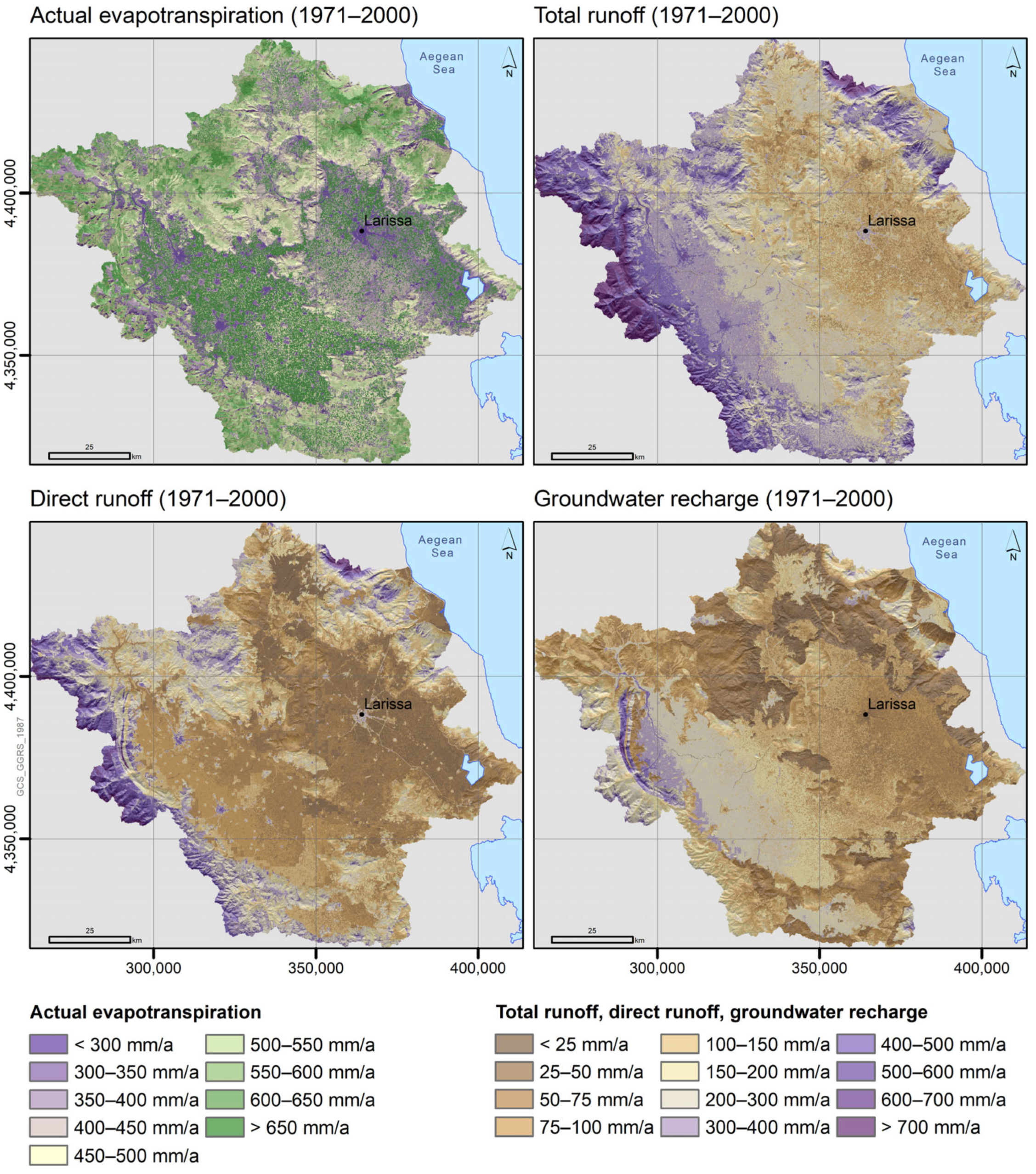
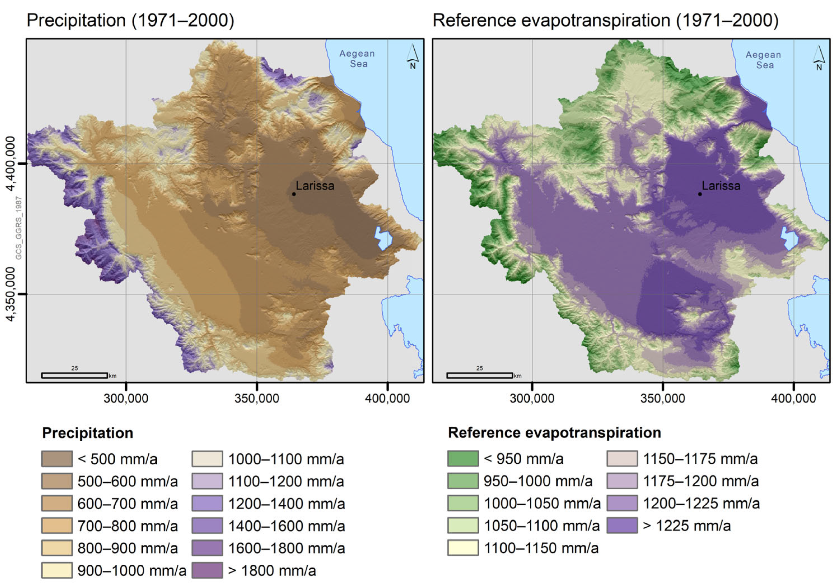
Maps of the long-term annual water balance quantities for water resources management purposes in the PRB were calculated by temporal aggregation of mGROWA’s grid-based simulation results. Figure 13 displays the spatial patterns of simulated mean annual actual evapotranspiration, total runoff, direct runoff, and groundwater recharge. Because actual evapotranspiration strongly depends on the water available in soil and impervious surface storages, the low water storage capacity of the ground surface and soil in urban areas, in combination with the number of rain days per year, is the reason for the low levels below 300 mm/a in these environments. In contrast, the high plant available field capacity of soils and irrigation application raise evapotranspiration significantly above the level of 650 mm/a over large areas of the agricultural plains. Forested areas in low and moderate slopes reach levels above 600 mm/a, whereas Mediterranean shrublands covering moderate to steep slopes as well as flat low-water-capacity soils exhibit mean evapotranspiration values in the range 400 to 550 mm/a.

Precipitation water that does not leave the basin as evapotranspiration is modelled as total runoff in mGROWA in the long-term. High total runoff occurs in mountainous terrain (>500 mm/a) and a general east-west gradient can be observed in the plains, with an increase from 100 to 300 mm/a. These quantities of water runoff follow different flow paths, according to the BFI values introduced in Figure 7 and Figure 8. Quick runoff (interflow, overland flow; considered as direct runoff) dominates in mountainous terrain, except in karstic areas. Direct runoff feeds the river systems in the PRB mainly during the hydrological winter half-year and is the main cause of the intermittent character of smaller creeks. Along the fringes of the mountain ranges, direct runoff seeps laterally into unconsolidated aquifers of the basins and acts as lateral aquifer recharge. The portion of the direct runoff that likely infiltrates into groundwater bodies via the streambeds has not been considered; however, major contributions to aquifer recharge originate from in-situ groundwater recharge, as shown in Figure 13.

The spatial distribution of groundwater recharge is governed by geologic properties, but also by the patterns of climatic quantities (mainly precipitation). The lowest recharge rates occur in the southern parts of the Eastern Thessaly plain, with values below 50 mm/a. In the north-western unconsolidated and highly permeable parts of the Western Thessaly plain, recharge levels can exceed 300 mm/a. Significant groundwater recharge also takes place in the karstic rock formations, with levels of 300 mm/a and higher.

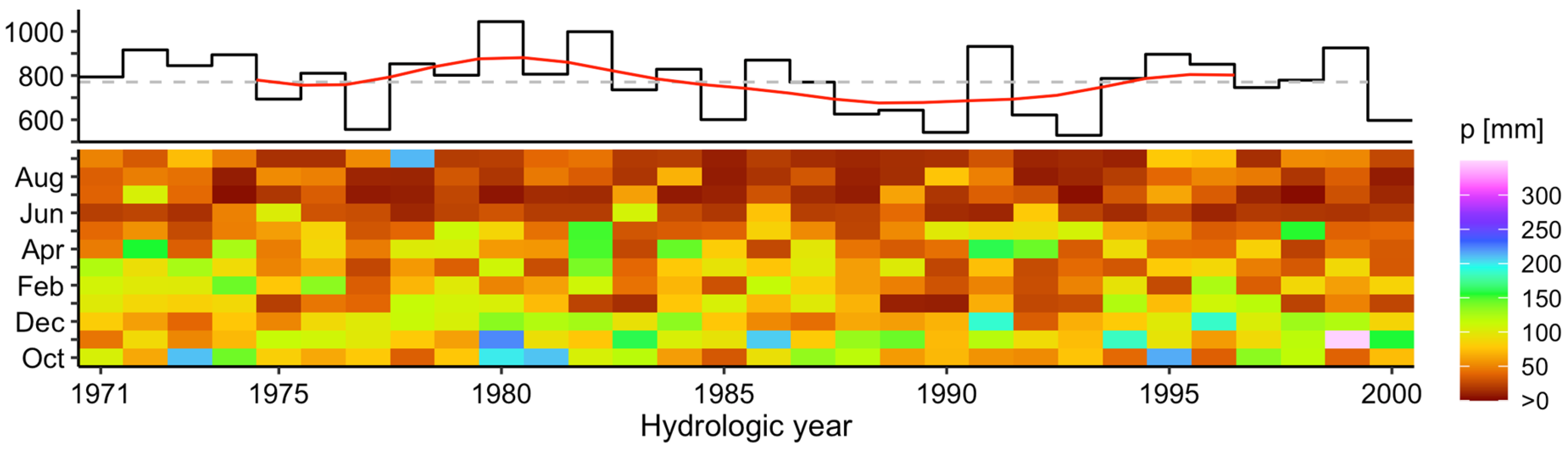
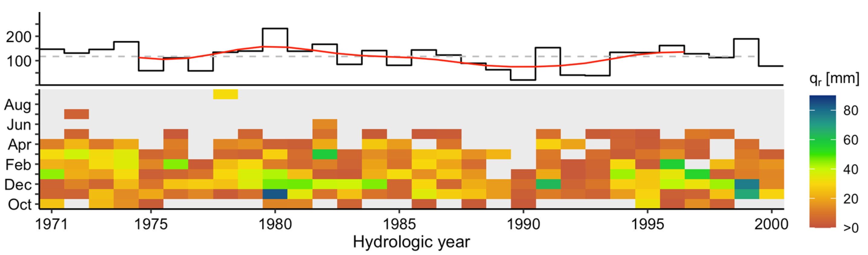
Figure 14 illustrates the temporal patterns of in-situ groundwater recharge aggregated for the whole PRB. As expected, recharge frequently occurs during the hydrologic winter half-year, with no simulated recharge occurring for the majority of the summer months. The interannual variability generally follows the precipitation patterns. The long-term catchment-averaged annual groundwater recharge amounts to approximately 120 mm/a. Monthly precipitation quantities that are close to the mean climatological level during winter half-year typically cause a low level of groundwater recharge of less than 20 mm/month. High groundwater recharge at the level of 50 mm/month and above occurs only when precipitation exceeds 150 mm/month, i.e., during above-average wet months and occasionally associated with extreme rain events. These events regularly lift the annual groundwater recharge above the long-term annual average, whereas more uniform temporal distributions of winter precipitation rarely lead to above-average levels.

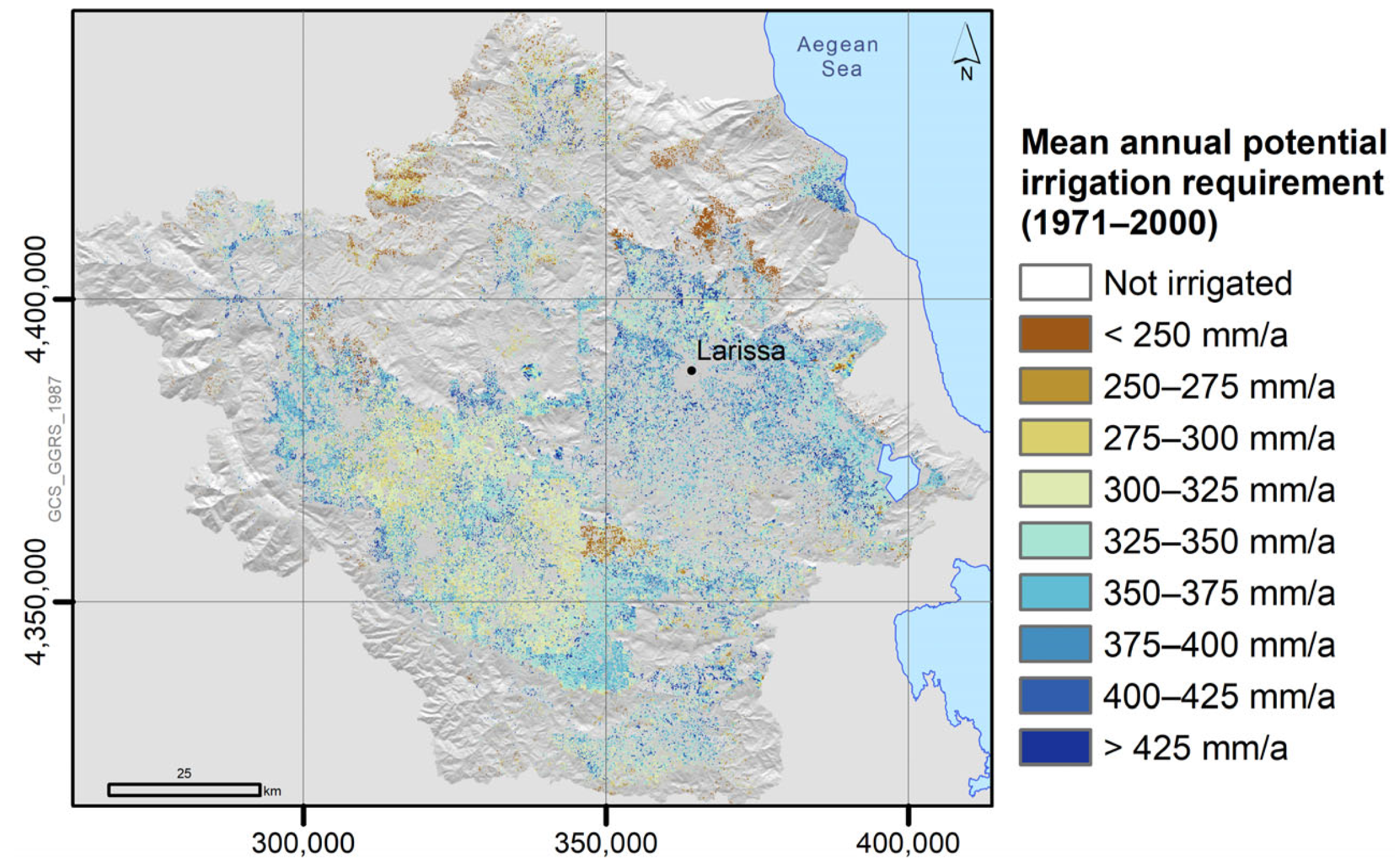
Figure 15 displays the spatial distribution of mean annual potential irrigation requirements (1971–2000) simulated using mGROWA, and

Table 5. Spatial statistics (in mm/a) of long-term annual potential irrigation requirements (1971–2000) in the PRB.

	Mean	Median	Interquartile Range	15th Percentile	85th Percentile
Vine	331	333	40	302	365
Olive	44	43	13	33	54
CCP 1	328	332	51	285	371
Corn	377	376	38	352	406
Alfalfa	407	411	59	367	457
Cotton	326	325	38	301	353

¹ Complex cultivation patterns.

provides the corresponding spatial statistics. Olives do not require extensive irrigation, whereas the other crops need multiple applications of irrigation per season, which result in long-term means ranging from 300 to more than 460 mm/a. The spatial patterns of the irrigation requirements are controlled by a combination of influencing factors; primarily by precipitation, plant available field capacity, and the irrigation rules.

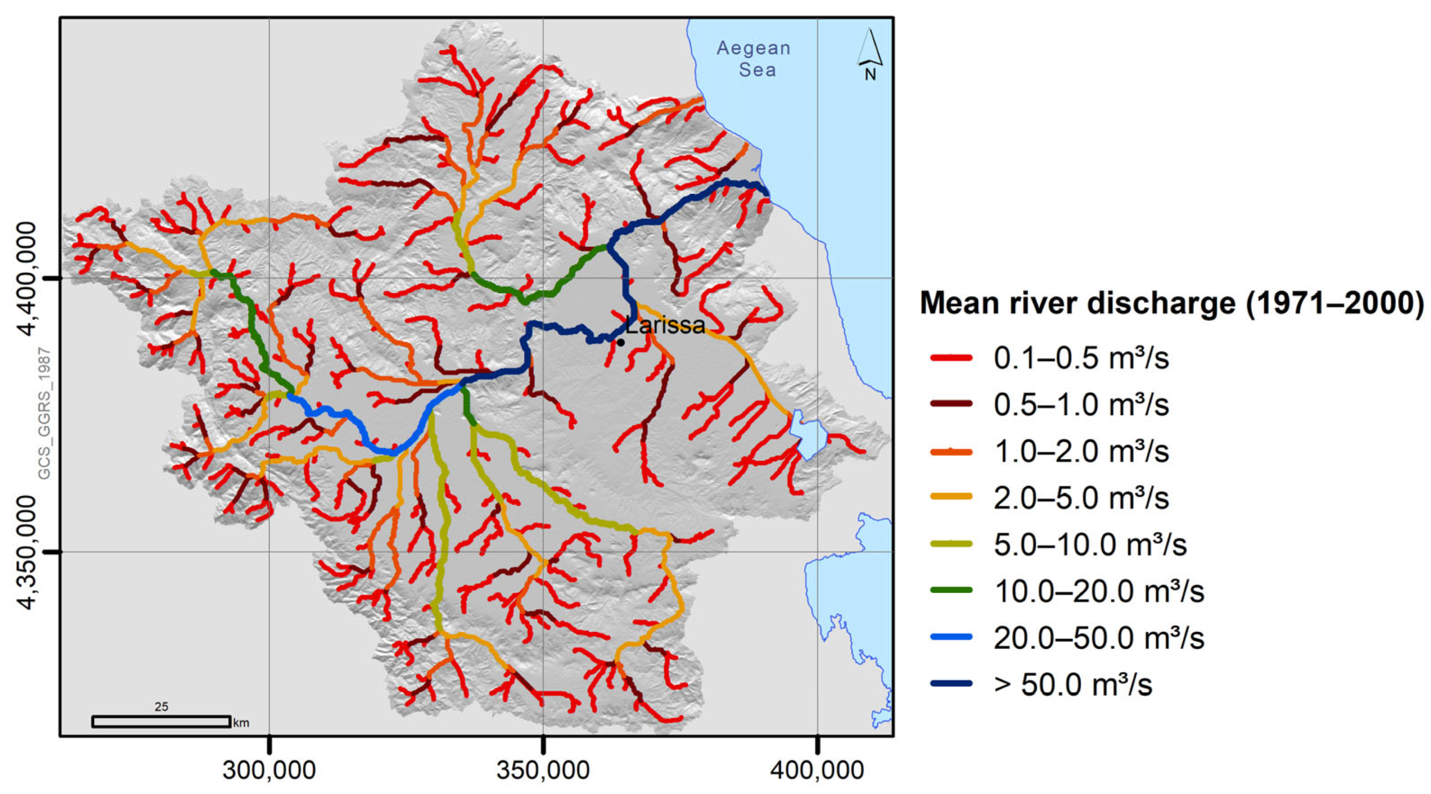
Figure 16 displays the simulated mean longitudinal river discharge for the period 1971–2000 under the assumptions of congruent surface and sub-surface catchments of the plotted river segments and largely natural discharge behaviour, i.e., no withdrawals for irrigation purposes, bypasses, wastewater inflows, etc. The approach implemented to calculate longitudinal river discharge profiles uses the total runoff pattern shown in Figure 13 and flow directions derived from the DEM (Figure 4). The flow accumulation is calculated using the fast algorithm proposed by Zhou et al. [84]. According to this approach, the Pinios River has a long-term mean discharge (1971–2000) of 89.9 m³/s at the outlet to the Aegean Sea.

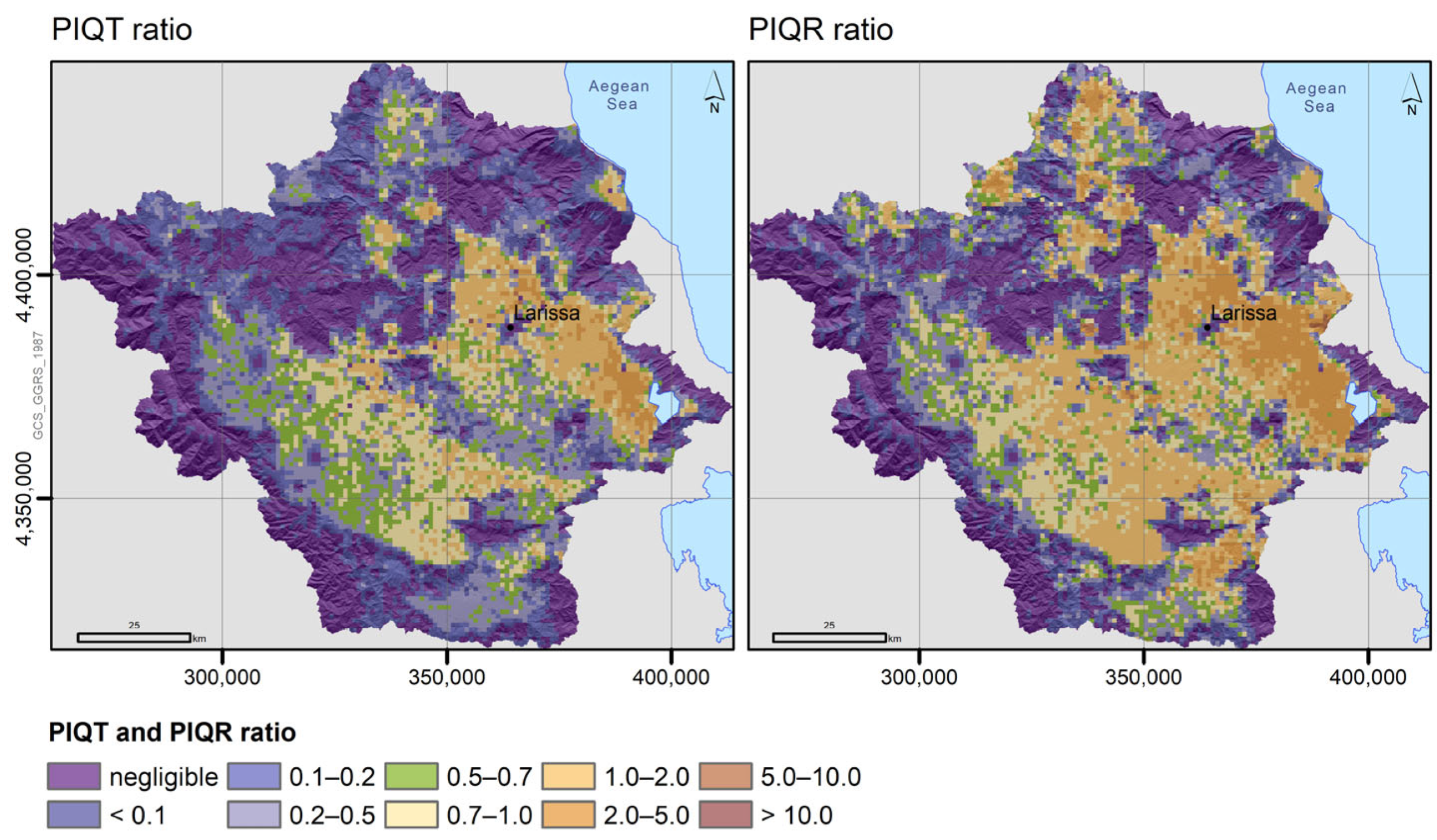
Bringing together the simulated irrigation requirements, which represent the potential irrigation requirements, and total runoff or groundwater recharge in practical indices allows insights into spatial patterns of water availability for agricultural purposes [15]. Figure 17 shows the spatial distribution of the ratio of potential irrigation to total runoff (PIQT ratio) and to groundwater recharge (PIQR ratio). These indices are calculated by applying the flow accumulation approach to the simulated variables, and then using the accumulated values at each grid cell to calculate the ratios. The ratios therefore depict the overall situation at each grid cell, including the situation topographically upstream. Values close to zero indicate zero or negligible water consumption by agriculture. Within the range 0 to 1, irrigation water consumption in the upstream areas can theoretically be supplied by the runoff or groundwater recharge formed upstream. However, in practice values around 0.7 seem to be thresholds in this context. The higher the values above 1 (or 0.7), the more water has to be transferred from other parts of the PRB to supply irrigation requirements. In the case of irrigated agriculture in the Pinios delta, the major part of required water quantities are extracted from the Pinios River [85] and were previously formed as discharge somewhere else in the headwaters of the river system.

The PIQT and PIQR also indirectly indicate the pressure on farmers to compete for water for irrigation. The hotspot of this competition for water resources is clearly the Eastern Thessaly basin. This is one of the main reasons for which the Lake Karla reservoir, in the southern part of the Eastern Thessaly basin (see Figure 2), was re-established [22]. The small mountain fringe around the Karla reservoir provides significant quantities of direct runoff which is used to counterbalance some of the water gap caused by the very low level of in-situ groundwater recharge observed there.

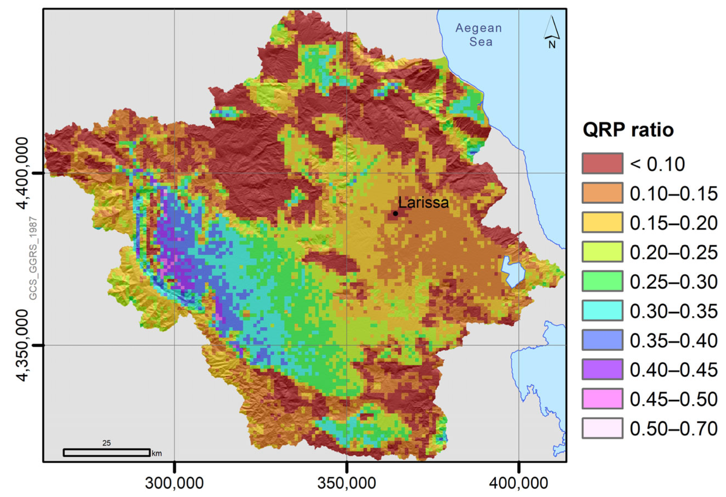
Additionally, from a water management perspective, the long-term groundwater recharge to precipitation ratio (QRP ratio) constitutes a useful indicator, as it provides spatial information about the percentage of precipitation that becomes groundwater recharge in years of average climate conditions. The QRP ratio was calculated based on the mGROWA simulation results and is shown in Figure 18. The highest ratios (>0.5) are attained in the Western Thessaly basin, whereas the Eastern Thessaly basin again shows low values, in particular at the south-eastern edge. Most of the mountain ranges also exhibit low ratios frequently below 0.1 (except the karstic units), because rock formations are of low permeability and cannot accommodate high amounts of groundwater recharge. As described above, interflow is the dominant runoff component at these sites.

6. Model Evaluation Strategy and Discussion

The evaluation of long-term water balance simulations covering a non-recent hydrologic period is challenging, particularly when river discharge gauges were not permanently installed and maintained in a basin. As in many regions, long, reliable, and continuous discharge hydrographs are rare for the PRB and hydrologic observation networks were downsized during the last decades. Furthermore, discharge values from the published literature do not necessarily match the hydrologic period modelled in this study. For example, Therianos [86] provided an average discharge of 80.92 m³/s (published in Foutrakis et al. [87]) in the Pinios estuary area, which was probably derived for below-average dry years in the 1960s. However, this value compares well to the long-term average (1971–2000) of 89.9 m³/s produced by mGROWA. Moreover, Migiros et al. [32] state that the mean annual total discharge is 3500 × 10⁶ m³ (equivalent to 111 m³/s), without naming sources, which appears to correspond to wet year conditions.

The common method to evaluate mGROWA simulations is to compare long-term mean observed discharge with simulated total runoff in a set of sub-catchments of a larger basin. For this purpose, observed discharge is converted from m³/s to catchment-averaged mm/a.

Table 6. River gauges and discharge values used for model evaluation.

Gauge	Long.	Lat.	Catchment Area in km2	Available Years	Mean Observed Discharge in m3/s	Reliability Assumption
Ali Efenti	22.07909	39.56958	2699	1960–1994	39.2	High
Amigdalia	22.25717	39.65873	6348	1974–1985	62.1	Low
Ampelia	22.52839	39.30903	626	1961–1985	2.8	Low
Gavros	21.60603	39.82118	230	1974–1985	1.5	Low
Kedros	22.03299	39.19899	493	1976–1981	6.4	Unknown
Larissa-Alkazar	22.41176	39.64145	7031	1961–1993	67.5	Low to Medium
Larissa-Giannouli	22.40774	39.65258
Piniada	22.16876	39.58671	6025	1983–1993	42.6	High
Sarakina	21.63311	39.66903	1042	1961–1984	13.9	Low
Skopia	22.47855	39.15106	369	1972–1993	1.7	High

lists the set of gauges (sub-catchments shown in Figure 19, right) that were selected from the results of research in the studies of HYDROMET [88], Zarris et al. [89], and Koutsogiannis et al. [90]. A quality flag describing the reliability of the streamflow data is also included in the Table 6, determined based on the detailed description of gauges included in the study of Zarris et al. [89]. Within the evaluation procedure, only periods with complete observed data were considered, except from only a very few cases in which filled data with double linear regression were obtained from the study of Koutsogiannis et al. [90].

This evaluation procedure is additionally impeded by the fact that water abstraction quantities from rivers and groundwater for irrigation purposes are unknown. Although the observed discharge implicitly accounts for water abstractions, the spatially distributed total runoff simulated in mGROWA does not in the same way, because a part of the simulated total runoff is transferred to irrigation internally within the sub-catchments. 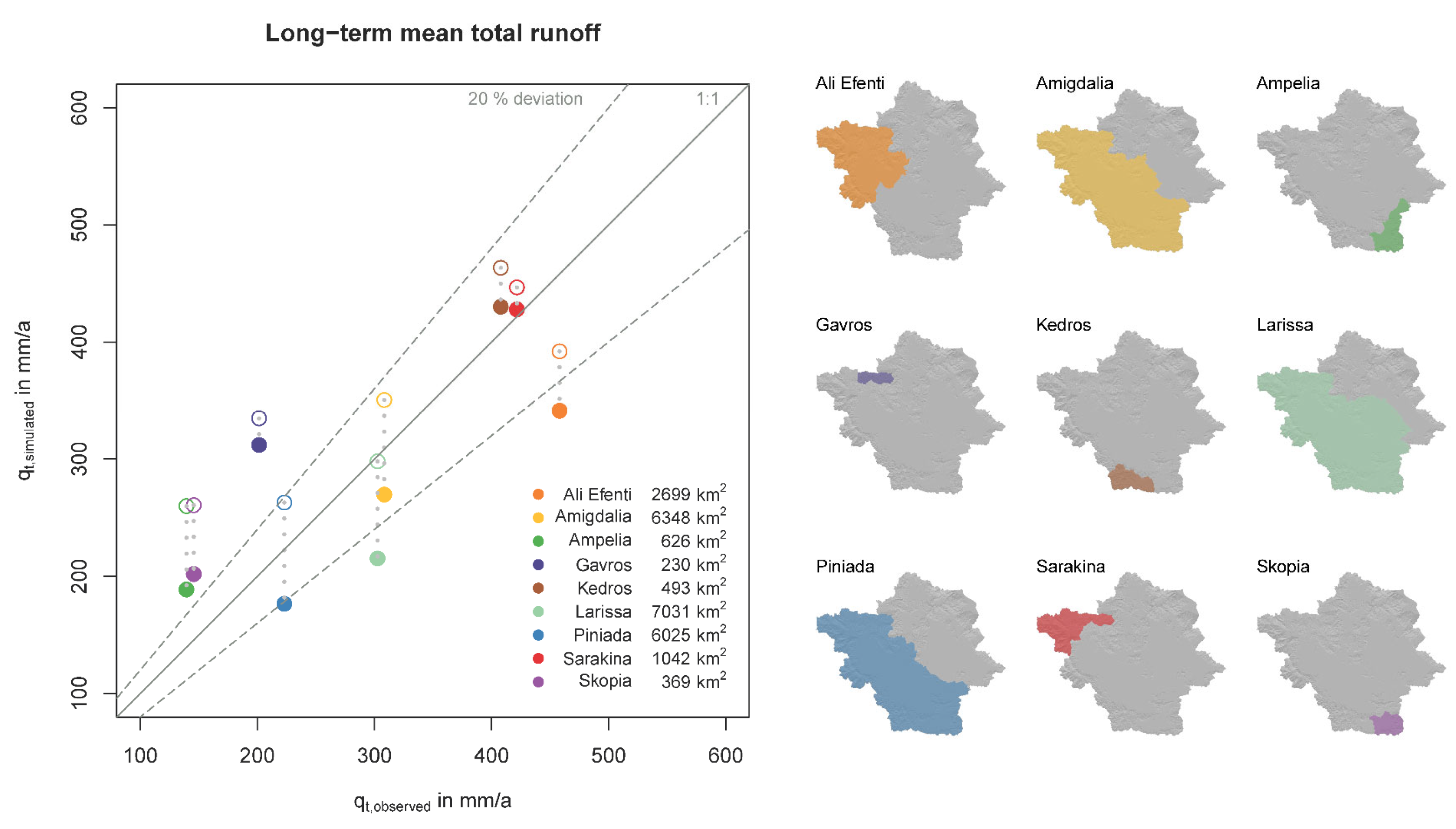To therefore correct these simulated runoff values and derive discharge values for a sub-catchment, a fraction (considered as a correction factor) of the simulated potential irrigation requirement (Figure 15) should be subtracted from the total simulated runoff. The values of the correction factors are catchment-specific and are unfortunately unknown. For this reason, we show the whole range of the possible influence of the correction factors in the scatter plot of results shown in Figure 19 (left), in which unfilled circles represent uncorrected simulated total runoff while filled circles represent 100% correction by simulated potential irrigation.

The results presented in Figure 19 suggest a tendency for the mGROWA model to overestimate the total runoff in smaller mountainous headwater sub-catchments such as Gavros, Skopia, Sarakina, Kedros, and Ampelia, where irrigation water consumption is generally lower than in the plains. The smaller range resulting from the correction process indicates these lower irrigation requirements. We hypothesise that one reason for this finding could be that the orographic gradients applied (see Section 4.4) could overestimate precipitation quantities in high altitudes; however, this would also influence the model performance at the downstream gauges. The large sub-catchments corresponding to the gauges Larissa (as the sum of Alkazar and Giannouli gauges), Piniada, and Amigdalia reveal a good agreement of the simulation and observation. This is indicated by the position of these points close to the 1:1-line and their linking lines (dotted) that intersect it. The knowledge of the true amount of irrigation water abstraction would likely lead to a very good model performance after application of the relevant correction factor. Consequently, we conclude that mGROWA has been proved to provide a reliable spatially distributed water balance of the PRB.

In contrast to the total runoff, the evaluation of groundwater recharge is even more challenging. In general, groundwater recharge in a basin can be equated with base flow over a long period. Behind this approach is the assumption that the inflow (recharge) and outflow (base flow) from an aquifer must be constant in the long-term if the level in the aquifer also remains constant. In practice, the base flow can be determined by filtering the hydrograph, however, this process requires daily streamflow data which were available only for the gauges in Larissa. The implementation of Arnold’s filtering method [91] in daily streamflow data from Larissa yielded a base-flow fraction of 0.54 in total discharge. This compares well with the value of 0.46 that can be derived from our mGROWA setup for the Larissa sub-catchment.

7. Summary and Future Research

The components of the water balance, most importantly the crop-specific potential irrigation requirements, actual evapotranspiration, total runoff, direct runoff, and groundwater recharge, were simulated using mGROWA for the PRB for 1971–2000. The established model setup comprises comprehensive observed climatic input data and spatially distributed parameters from national and European datasets. The derivation of reliable geomorphologically plausible parameter distributions (BFI values, plant available field capacity, etc.) posed a key challenge in the study.

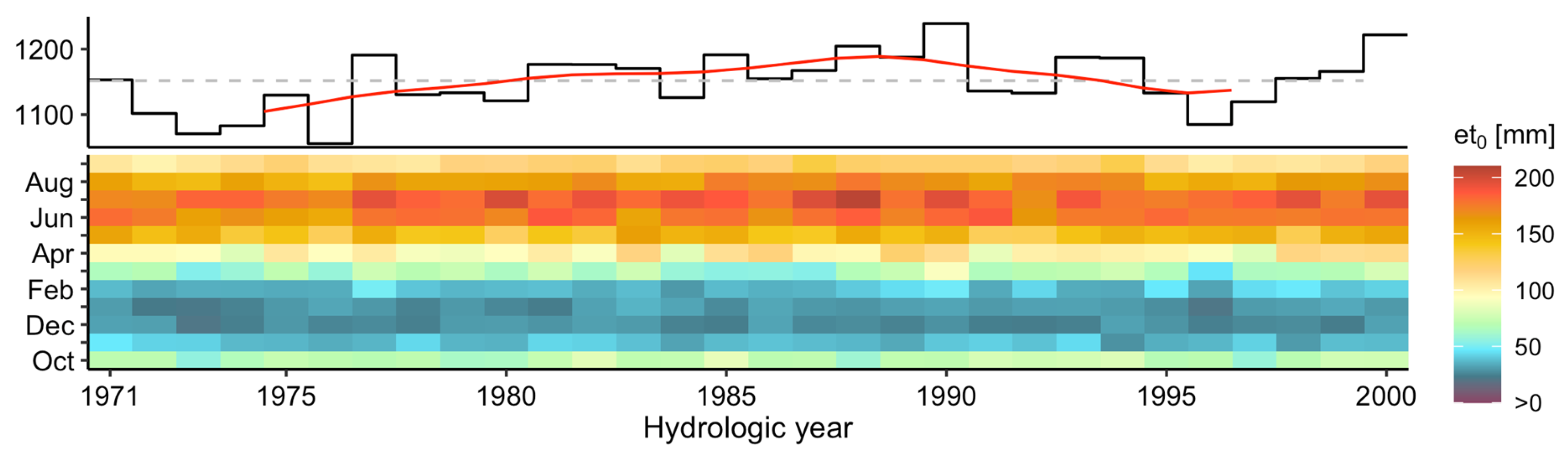
A trend of increasing reference evapotranspiration in the range of 1050 to 1200 mm/a has been observed in the PRB in the period 1971–2000, while the precipitation time series shows an extended dry period from 1988 until 1993, but without a noticeable long-term trend. The long-term catchment-averaged annual potential irrigation requirements of the major crops cultivated in the PRB varies from 300 to more than 460 mm/a. Comparing to other studies, our results are reasonable for the major crops of the PRB. More in detail, Tsakmakis et al. [92] presented that irrigation water requirements calculated with crop growth modelling and applied in cotton fields located in North Greece ranged between 227 mm (deficit irrigation applied with drip system) and 400 mm (regular irrigation applied with sprinkler system). Stamatiadis et al. [93] reported that intermediate irrigation was 300 and 335 mm for cotton fields located in the PRB (near Larissa) for years 2008 and 2009, respectively. For a corn cultivation field located in the Pinios River Basin, Tsakmakis et al. [94] indicated irrigation requirements of 350 mm based on crop growth modelling. Nevertheless, according to the water district management plan [35], cotton irrigation requirements were found to range between 427 and 445 mm. These requirements are significantly higher than the average cotton irrigation requirements presented in Table 5. This discrepancy is mainly attributed to the different approach in calculating crop irrigation requirements. Irrigation water requirements reported in the water district management plan [35] are calculated according to the Greek Ministerial Decision No. Φ.16/6631 (JoG issue B’ 428 2/6/1989) “Estimation of the minimum and maximum necessary volumes for the rational use of water in irrigation”, which is based on the Blaney–Criddle formula [95]. According to Tegos et al. [96], this formula was found to overestimate the potential evapotranspiration by 30% in Greece, while for stations located far from the sea, such as Larissa, the deviation was found to exceed 50%. Moreover, cotton irrigation requirements reported in the water district management plan imply full irrigation, while our approach is based on moderate deficit irrigation of cotton. Similar or higher discrepancies in irrigation water requirements are also presented for the other crops. These differences are partially reflected at the basin scale, since the 814 hm³ of average annual potential irrigation water demand simulated with mGROWA for the irrigated agricultural land of the PRB is substantially less than the 1202.5 hm³ reported in the water district management plan [35]. Aside from the different irrigation water requirement calculation methodologies, this difference can be also attributed to the following factors: (1) our calculations do not incorporate the efficiency of irrigation systems and losses of water distribution, meaning that they can be considered to be close to the optimal and (2) for cotton and complex cultivation patterns, moderate deficit irrigation is applied with mGROWA, which reduces the irrigation water requirements on the basin scale.

The extraction of these water volumes from the ground and surface waters places substantial stress on the water resources of the basin. The groundwater resources of the basin are recharged at a mean rate of approximately 120 mm/a. In line with the long-term temporal patterns of precipitation, there was no obvious temporal trend in groundwater recharge in the PRB from 1971 to 2000, but groundwater recharge declined corresponding to the extended dry period from 1988 until 1993. The mGROWA simulation provides additional data for further analyses and comprehensive statistics in terms of water resources management, e.g., the PIQT and PIQR ratios. The procedure applied to evaluate the total runoff simulated by mGROWA revealed the uncertainties associated with modelling in data-scarce basins, such as the PRB. There are several starting points to improve, proceed and extend the water balance modelling in the PRB in addition to the findings achieved so far, some of which are briefly discussed in the following paragraphs.

Due to the grid-based 1-D nature of the mGROWA model, simulation results require some post-processing in a GIS-system or numerical groundwater model to derive final key parameters for decisions in water resources management (e.g., to derive the sustainably usable groundwater supply in a groundwater body). In the case of the PRB, interflow as a component of direct runoff seeps laterally into unconsolidated aquifers of the basins along the fringes of mountain ranges and acts as lateral recharge of the main aquifer. Thus, the total aquifer recharge of the main aquifers in the two Thessaly plains consists of this lateral component, in-situ groundwater recharge in the plains and other difficult to estimate influxes over various boundaries. In practice, the water volumes and rates calculated using mGROWA can serve as boundary conditions in more specific groundwater modelling studies, as described in Herrmann et al. [97]. Nevertheless, simulation results from mGROWA have been proven to provide reliable decision support for water resources management at the regional scale, e.g., recently in the federal state of Lower Saxony (Germany) [14] and the Ergene River Basin (Turkey) [18].

In addition to the application of mGROWA to provide data on total water fluxes for water resources management, the model has been established in a model chain together with a regional-scale nutrient model (mGROWA-DENUZ) In the Thessaly Water District, nitrates constitute a diffuse pollution from agricultural activities that should be controlled and mitigated [98]. The ongoing implementation of the already established action plans in Thessaly would benefit from results of the model chain mGROWA-DENUZ.

In the context of the present study, we provide a comprehensive description of parameterisation workflow, adapted to the data availability situation in Greece. This workflow can be used as a guidance for the implementation of fully distributed water balance models in European data-scarce regions, since the data used are usually available under public domain. Nevertheless, and as described in this article, further improvements to the input datasets are needed to advance the model’s reliability. It is widely known that the Mediterranean region is prone to severe observation data scarcity. For this reason, the Pinios Hydrologic Observatory (PHO) [99] was established to improve data availability in the eastern part of the PRB and to support the improvement of parameter estimations, which are of fundamental importance for water balance modelling in the Mediterranean region [49]. In the PHO, for example, several observation sites at the southern slopes of the Mount Ossa massif have been equipped with various meteorological and soil moisture sensors. They almost completely cover the range of elevation levels in the region and can support, among other things, increased accuracy in the calculation of the orographic gradients of precipitation and reference evapotranspiration described in Section 4.4.

To complement the model performance evaluation presented in our study, we propose additional methods for evaluation in future studies. Model performance evaluation will continue to be an issue in forthcoming studies. We plan to evaluate simulated soil moisture time series (mGROWA MLSM) by comparing simulated soil moisture time series with the advanced remote sensing products described in El Hajj et al. [100] and Bazzi et al. [101], using an approach similar to Herrmann et al. [17]. Additionally, for the evaluation of simulated total runoff and baseflow, improvements in model evaluation might be difficult to achieve, since the current river flow monitoring network is not able to support such a task. Nevertheless, analysing reconstructed historical hydrographs in combination with a modern powerful hydrograph filter (e.g., described in Pelletier and Andréassian [102]) can provide information to support the suitability of the BFI values chosen for this study.

A major obstacle to the efficient water resources management in the PRB is the non-existence of short-term retrospective and forecasting water balance simulations, which could quantify, for example, the severity and impacts of water scarcity events. The meteorological observation network in the PRB has shrunk over the previous decades and the gridded E-OBS data (ENSEMBLES daily gridded observational dataset for precipitation, temperature and sea level pressure in Europe [103,104]) show many gaps over the PRB model domain. A possible approach to accurately characterise the spatiotemporal patterns of meteorological data from 2000 onwards seems to be the use of reanalysis data (e.g., COSMO-REA6 [105]) in a model chain with mGROWA. As a mid-term goal, the full operational mode of mGROWA is intended to encompass the coupling with numerical weather forecast models.

Numerous studies have stated that irrigation water requirements are expected to increase [106] and available freshwater resources to decrease [107] in the Mediterranean region due to climate change. A reduction in mean annual precipitation in the PRB of 80 mm/a is expected by 2100 [34]. Several studies have already demonstrated the suitability of implementing mGROWA for climate change impact studies [15,17,108]. Consequently, such a study using mGROWA in a chain with the EURO-CORDEX RCM ensemble [29] is the next reasonable step towards providing the data basis for developing strategies for future water resources management in the PRB.

References

1. Giorgi, F. Climate change hot-spots. Geophys. Res. Lett. 2006, 33, L08707. [Google Scholar] [CrossRef]
2. Hoerling, M.; Eischeid, J.; Perlwitz, J.; Quan, X.; Zhang, T.; Pegion, P. On the Increased Frequency of Mediterranean Drought. J. Clim. 2012, 25, 2146–2161. [Google Scholar] [CrossRef] [Green Version]
3. La Jeunesse, I.; Cirelli, C.; Aubin, D.; Larrue, C.; Sellami, H.; Afifi, S.; Bellin, A.; Benabdallah, S.; Bird, D.N.; Deidda, R.; et al. Is climate change a threat for water uses in the Mediterranean region? Results from a survey at local scale. Sci. Total Environ. 2016, 543, 981–996. [Google Scholar] [CrossRef]
4. Nastos, P.T.; Zerefos, C.S. Climate Change and precipitation in Greece. Hell. J. Geosci. 2010, 45, 185–192. [Google Scholar]
5. Pnevmatikos, J.D.; Katsoulis, B.D. The changing rainfall regime in Greece and its impact on climatological means. Meteorol. Appl. 2006, 13, 331–345. [Google Scholar] [CrossRef]
6. Hatzianastassiou, N.; Katsoulis, B.; Pnevmatikos, J.; Antakis, V. Spatial and Temporal Variation of Precipitation in Greece and Surrounding Regions Based on Global Precipitation Climatology Project Data. J. Clim. 2008, 21, 1349–1370. [Google Scholar] [CrossRef]
7. García-Ruiz, J.M.; López-Moreno, J.I.; Vicente-Serrano, S.M.; Lasanta–Martínez, T.; Beguería, S. Mediterranean water resources in a global change scenario. Earth-Sci. Rev. 2011, 105, 121–139. [Google Scholar] [CrossRef] [Green Version]
8. Milly, P.C.; Betancourt, J.; Falkenmark, M.; Hirsch, R.M.; Kundzewicz, Z.W.; Lettenmaier, D.P.; Stouffer, R.J. Climate change. Stationarity is dead: Whither water management? Science 2008, 319, 573–574. [Google Scholar] [CrossRef]
9. Mimikou, M.A.; Baltas, E.A. Assessment of Climate Change Impacts in Greece: A General Overview. Am. J. Clim. Chang. 2013, 2, 46–56. [Google Scholar] [CrossRef]
10. Destouni, G.; Prieto, C. Robust Assessment of Uncertain Freshwater Changes: The Case of Greece with Large Irrigation—And Climate-Driven Runoff Decrease. Water 2018, 10, 1645. [Google Scholar] [CrossRef] [Green Version]
11. Refsgaard, J.C.; Madsen, H.; Andréassian, V.; Arnbjerg-Nielsen, K.; Davidson, T.A.; Drews, M.; Hamilton, D.P.; Jeppesen, E.; Kjellström, E.; Olesen, J.E.; et al. A framework for testing the ability of models to project climate change and its impacts. Clim. Chang. 2014, 122, 271–282. [Google Scholar] [CrossRef] [Green Version]
12. Medici, C.; Butturini, A.; Bernal, S.; Vázquez, E.; Sabater, F.; Vélez, J.I.; Francés, F. Modelling the non-linear hydrological behaviour of a small Mediterranean forested catchment. Hydrol. Process. 2008, 22, 3814–3828. [Google Scholar] [CrossRef]
13. Herrmann, F.; Keller, L.; Kunkel, R.; Vereecken, H.; Wendland, F. Determination of spatially differentiated water balance components including groundwater recharge on the Federal State level—A case study using the mGROWA model in North Rhine-Westphalia (Germany). J. Hydrol. Reg. Stud. 2015, 4, 294–312. [Google Scholar] [CrossRef] [Green Version]
14. Ertl, G.; Herrmann, F.; Elbracht, J. Determination of groundwater recharge for solid rock areas in Lower Saxony. Grundwasser 2022, 27, 43–56. [Google Scholar] [CrossRef]
15. Herrmann, F.; Kunkel, R.; Ostermann, U.; Vereecken, H.; Wendland, F. Projected impact of climate change on irrigation needs and groundwater resources in the metropolitan area of Hamburg (Germany). Environ. Earth Sci. 2016, 75, 1104. [Google Scholar] [CrossRef]
16. Ehlers, L.; Herrmann, F.; Blaschek, M.; Duttmann, R.; Wendland, F. Sensitivity of mGROWA-simulated groundwater recharge to changes in soil and land use parameters in a Mediterranean environment and conclusions in view of ensemble-based climate impact simulations. Sci. Total Environ. 2016, 543, 937–951. [Google Scholar] [CrossRef]
17. Herrmann, F.; Baghdadi, N.; Blaschek, M.; Deidda, R.; Duttmann, R.; La Jeunesse, I.; Sellami, H.; Vereecken, H.; Wendland, F. Simulation of future groundwater recharge using a climate model ensemble and SAR-image based soil parameter distributions—A case study in an intensively-used Mediterranean catchment. Sci. Total Environ. 2016, 543, 889–905. [Google Scholar] [CrossRef] [PubMed]
18. Rukundo, E.; Doğan, A. Dominant Influencing Factors of Groundwater Recharge Spatial Patterns in Ergene River Catchment, Turkey. Water 2019, 11, 653. [Google Scholar] [CrossRef] [Green Version]
19. Vasiliades, L.; Loukas, A.; Liberis, N. A Water Balance Derived Drought Index for Pinios River Basin, Greece. Water Resour. Manag. 2011, 25, 1087–1101. [Google Scholar] [CrossRef]
20. Panagopoulos, Y.; Makropoulos, C.; Gkiokas, A.; Kossida, M.; Evangelou, L.; Lourmas, G.; Michas, S.; Tsadilas, C.; Papageorgiou, S.; Perleros, V.; et al. Assessing the cost-effectiveness of irrigation water management practices in water stressed agricultural catchments: The case of Pinios. Agric. Water Manag. 2014, 139, 31–42. [Google Scholar] [CrossRef]
21. Panagopoulos, Y.; Makropoulos, C.; Kossida, M.; Mimikou, M. Optimal Implementation of Irrigation Practices: Cost-Effective Desertification Action Plan for the Pinios Basin. J. Water Resour. Plan. Manag. 2014, 140, 05014005. [Google Scholar] [CrossRef]
22. Loukas, A.; Mylopoulos, N.; Vasiliades, L. A Modeling System for the Evaluation of Water Resources Management Strategies in Thessaly, Greece. Water Resour. Manag. 2007, 21, 1673–1702. [Google Scholar] [CrossRef]
23. Loukas, A. Surface water quantity and quality assessment in Pinios River, Thessaly, Greece. Desalination 2010, 250, 266–273. [Google Scholar] [CrossRef]
24. Stefanidis, K.; Panagopoulos, Y.; Psomas, A.; Mimikou, M. Assessment of the natural flow regime in a Mediterranean river impacted from irrigated agriculture. Sci. Total Environ. 2016, 573, 1492–1502. [Google Scholar] [CrossRef]
25. Stefanidis, K.; Panagopoulos, Y.; Mimikou, M. Response of a multi-stressed Mediterranean river to future climate and socio-economic scenarios. Sci. Total Environ. 2018, 627, 756–769. [Google Scholar] [CrossRef] [PubMed]
26. Panagopoulos, A.; Arampatzis, G.; Kuhr, P.; Kunkel, R.; Tziritis, E.; Wendland, F. Area-differentiated modeling of water balance in Pinios Basin, central Greece. Glob. NEST J. 2015, 17, 221–235. [Google Scholar] [CrossRef]
27. Panagopoulos, A.; Arampatzis, G.; Tziritis, E.; Pisinaras, V.; Herrmann, F.; Kunkel, R.; Wendland, F. Assessment of climate change impact in the hydrological regime of River Pinios Basin, central Greece. Desalination Water Treat. 2016, 57, 2256–2267. [Google Scholar] [CrossRef]
28. Evangelou, E.; Tsadilas, C.; Tserlikakis, N.; Tsitouras, A.; Kyritsis, A. Water Footprint of Industrial Tomato Cultivations in the Pinios River Basin: Soil Properties Interactions. Water 2016, 8, 515. [Google Scholar] [CrossRef] [Green Version]
29. Jacob, D.; Petersen, J.; Eggert, B.; Alias, A.; Christensen, O.B.; Bouwer, L.M.; Braun, A.; Colette, A.; Déqué, M.; Georgievski, G.; et al. EURO-CORDEX: New high-resolution climate change projections for European impact research. Reg. Environ. Chang. 2014, 14, 563–578. [Google Scholar] [CrossRef]
30. Baltas, E.A. A new approach for the determination of hydrologic prefectures in Greece for the water framework directive. NEW MEDIT 2008, 3, 41–47. [Google Scholar]
31. European Commission. Report on the Implementation of the Water Framework Directive River Basin Management Plans—Member State: Greece. Commission Staff Working Document SWD(2015) 54; European Commission: Brussels, Belgium, 2015. [Google Scholar]
32. Migiros, G.; Bathrellos, G.; Skilodimou, H.; Karamousalis, T. Pinios (Peneus) River (Central Greece): Hydrological—Geomorphological elements and changes during the quaternary. Open Geosci. 2011, 3, 215–228. [Google Scholar] [CrossRef]
33. Beck, H.E.; Zimmermann, N.E.; McVicar, T.R.; Vergopolan, N.; Berg, A.; Wood, E.F. Present and future Koppen-Geiger climate classification maps at 1-km resolution. Sci. Data 2018, 5, 180214. [Google Scholar] [CrossRef] [Green Version]
34. Arampatzis, G.; Panagopoulos, A.; Pisinaras, V.; Tziritis, E.; Wendland, F. Identifying potential effects of climate change on the development of water resources in Pinios River Basin, Central Greece. Appl. Water Sci. 2018, 8, 51. [Google Scholar] [CrossRef] [Green Version]
35. Hellenic Special Secretariat for Water. Water Resouces Management Plan of Thessaly Water District, 1st Revision; Hellenic Ministry of Environment and Energy: Athens, Greece, 2017; p. 260. [Google Scholar]
36. Gemitzi, A.; Lakshmi, V. Evaluating Renewable Groundwater Stress with GRACE Data in Greece. Ground Water 2018, 56, 501–514. [Google Scholar] [CrossRef] [PubMed]
37. Kotsopoulos, S.; Alexiou, I.; Lokkas, P.; Kalfountzos, D.; Gravanis, G.; Magalios, S. Reliability of the reservoirs at the region of the former lake Karla in Thessaly in meeting crop water requirements. In Proceedings of the EWRA Seventh International Conference, Limassol, Cyprus, 25–27 June 2009; pp. 619–625. [Google Scholar]
38. Panagopoulos, Y.; Dimitriou, E. A Large-Scale Nature-Based Solution in Agriculture for Sustainable Water Management: The Lake Karla Case. Sustainability 2020, 12, 6761. [Google Scholar] [CrossRef]
39. Tzabiras, J.; Vasiliades, L.; Sidiropoulos, P.; Loukas, A.; Mylopoulos, N. Evaluation of Water Resources Management Strategies to Overturn Climate Change Impacts on Lake Karla Watershed. Water Resour. Manag. 2016, 30, 5819–5844. [Google Scholar] [CrossRef]
40. Kunkel, R.; Wendland, F. The GROWA98 model for water balance analysis in large river basins—The river Elbe case study. J. Hydrol. 2002, 259, 152–162. [Google Scholar] [CrossRef]
41. Allen, R.G.; Pereira, L.S.; Raes, D.; Smith, M. Crop Evapotranspiration—Guidelines for Computing Crop Water Requirements; FAO—Food and Agriculture Organization of the United Nations: Rome, Italy, 1998. [Google Scholar]
42. Disse, M. Modellierung der Verdunstung und der Grundwasserneubildung in Ebenen Einzugsgebieten. Ph.D. Thesis, Fakultät für Bauingenieur- und Vermessungswesen der Universität Fridericiana zu Karlsruhe (TH), Karlsruhe, Germany, 1995. [Google Scholar]
43. Haberlandt, U.; Klöcking, B.; Krysanova, V.; Becker, A. Regionalisation of the base flow index from dynamically simulated flow components—A case study in the Elbe River Basin. J. Hydrol. 2001, 248, 35–53. [Google Scholar] [CrossRef]
44. Jarvis, A.; Reuter, H.I.; Nelson, A.; Guevara, E. Hole-Filled Seamless SRTM Data V4; International Centre for Tropical Agriculture (CIAT): Palmira, Colombia, 2008. [Google Scholar]
45. Hiederer, R. Mapping Soil Properties for Europe–Spatial Representation of Soil Database Attributes; Publications Office of the European Union: Luxembourg, 2013. [Google Scholar]
46. Panagos, P. The European soil database. GEO Connex. 2006, 5, 32–33. [Google Scholar]
47. Panagos, P.; Van Liedekerke, M.; Jones, A.; Montanarella, L. European Soil Data Centre: Response to European policy support and public data requirements. Land Use Policy 2012, 29, 329–338. [Google Scholar] [CrossRef]
48. Bornovas, J.; Rondogianni-Tsiambaou, T. Geological Map of Greece 1:500,000; Institute of Geology and Mineral Exploration: Athens, Greece, 1983. [Google Scholar]
49. Ludwig, R.; Roson, R. Climate change, water and security in the Mediterranean: Introduction to the special issue. Sci. Total Environ. 2016, 543, 847–850. [Google Scholar] [CrossRef] [PubMed]
50. ATV-DVWK. Verdunstung in Bezug zu Landnutzung, Bewuchs und Boden; Deutsche Vereinigung für Wasserwirtschaft, Abwasser und Abfall e.V.: Hennef, Germany, 2002; Volume 504. [Google Scholar]
51. Lazzara, P.; Rana, G. The use of crop coefficient approach to estimate actual evapotranspiration: A critical review for major crops under Mediterranean climate. Ital. J. Agrometeorol. 2010, 15, 25–39. [Google Scholar]
52. Allen, R.G.; Pruitt, W.O.; Raes, D.; Smith, M.; Pereira, L.S. Estimating Evaporation from Bare Soil and the Crop Coefficient for the Initial Period Using Common Soils Information. J. Irrig. Drain. Eng. 2005, 131, 14–23. [Google Scholar] [CrossRef]
53. Müller, U.; Waldeck, A. Auswertungsmethoden im Bodenschutz; Landesamt für Bergbau, Energie und Geologie Niedersachsen: Henner, Germany, 2011. [Google Scholar]
54. Webster, R.; Oliver, M.A. Geostatistics for Environmental Scientists; John Wiley & Sons, Ltd. Chichester: New York, NY, USA; Weinheim, Germany; Brisbane, Australia; Singapore; Toronto, ON, Canada, 2001. [Google Scholar]
55. Wackernagel, H. Multivariate Geostatistics; Springer-Verlag: Berlin/Heidelberg, Germany, 1995. [Google Scholar]
56. Dingman, S.L. Physical Hydrology, 2nd ed.; Prentice-Hall, Inc.: Upper Saddle River, NJ, USA, 2002. [Google Scholar]
57. De Reu, J.; Bourgeois, J.; Bats, M.; Zwertvaegher, A.; Gelorini, V.; De Smedt, P.; Chu, W.; Antrop, M.; De Maeyer, P.; Finke, P.; et al. Application of the topographic position index to heterogeneous landscapes. Geomorphology 2013, 186, 39–49. [Google Scholar] [CrossRef]
58. Weiss, A.D. Topographic position and landforms analysis. In Proceedings of the ESRI User Conference 2001, San Diego, CA, USA, 9–13 July 2001; pp. 227–245. [Google Scholar]
59. Conrad, O.; Bechtel, B.; Bock, M.; Dietrich, H.; Fischer, E.; Gerlitz, L.; Wehberg, J.; Wichmann, V.; Böhner, J. System for Automated Geoscientific Analyses (SAGA) v. 2.1.4. Geosci. Model Dev. 2015, 8, 1991–2007. [Google Scholar] [CrossRef] [Green Version]
60. Worthington, S.R.H.; Davies, G.J.; Alexander, E.C. Enhancement of bedrock permeability by weathering. Earth-Sci. Rev. 2016, 160, 188–202. [Google Scholar] [CrossRef]
61. Tetzlaff, B.; Andjelov, M.; Kuhr, P.; Uhan, J.; Wendland, F. Model-based assessment of groundwater recharge in Slovenia. Environ. Earth Sci. 2015, 74, 6177–6192. [Google Scholar] [CrossRef]
62. Bloomfield, J.P.; Allen, D.J.; Griffiths, K.J. Examining geological controls on baseflow index (BFI) using regression analysis: An illustration from the Thames Basin, UK. J. Hydrol. 2009, 373, 164–176. [Google Scholar] [CrossRef] [Green Version]
63. Caputo, R.; Bravard, J.-P.; Helly, B. The Pliocene-Quaternary tecto-sedimentary evolution of the Larissa Plain (Eastern Thessaly, Greece). Geodin. Acta 1994, 7, 219–231. [Google Scholar] [CrossRef]
64. Caputo, R.; Pavlides, S. Late Cainozoic geodynamic evolution of Thessaly and surroundings (central-northern Greece). Tectonophysics 1993, 223, 339–362. [Google Scholar] [CrossRef]
65. Kontogianni, V.; Pytharouli, S.; Stiros, S. Ground subsidence, Quaternary faults and vulnerability of utilities and transportation networks in Thessaly, Greece. Environ. Geol. 2006, 52, 1085–1095. [Google Scholar] [CrossRef]
66. Apostolidis, E.; Koukis, G. Engineering-geological conditions of the formations in the Western Thessaly basin, Greece. Open Geosci. 2013, 5, 407–422. [Google Scholar] [CrossRef] [Green Version]
67. Zomlot, Z.; Verbeiren, B.; Huysmans, M.; Batelaan, O. Spatial distribution of groundwater recharge and base flow: Assessment of controlling factors. J. Hydrol. Reg. Stud. 2015, 4, 349–368. [Google Scholar] [CrossRef] [Green Version]
68. Kling, H.; Nachtnebel, H.P. A method for the regional estimation of runoff separation parameters for hydrological modelling. J. Hydrol. 2009, 364, 163–174. [Google Scholar] [CrossRef]
69. Hargreaves, G.H.; Samani, Z.A. Reference Crop Evapotranspiration from Temperature. Appl. Eng. Agric. 1985, 1, 96–99. [Google Scholar] [CrossRef]
70. Rolland, C. Spatial and Seasonal Variations of Air Temperature Lapse Rates in Alpine Regions. J. Clim. 2003, 16, 1032–1046. [Google Scholar] [CrossRef]
71. Marquínez, J.; Lastra, J.; García, P. Estimation models for precipitation in mountainous regions: The use of GIS and multivariate analysis. J. Hydrol. 2003, 270, 1–11. [Google Scholar] [CrossRef]
72. Martínez-Cob, A. Multivariate geostatistical analysis of evapotranspiration and precipitation in mountainous terrain. J. Hydrol. 1996, 174, 19–35. [Google Scholar] [CrossRef] [Green Version]
73. Wagner, P.D.; Fiener, P.; Wilken, F.; Kumar, S.; Schneider, K. Comparison and evaluation of spatial interpolation schemes for daily rainfall in data scarce regions. J. Hydrol. 2012, 464–465, 388–400. [Google Scholar] [CrossRef]
74. Vicente-Serrano, S.M.; Azorin-Molina, C.; Sanchez-Lorenzo, A.; Revuelto, J.; Morán-Tejeda, E.; López-Moreno, J.I.; Espejo, F. Sensitivity of reference evapotranspiration to changes in meteorological parameters in Spain (1961–2011). Water Resour. Res. 2014, 50, 8458–8480. [Google Scholar] [CrossRef] [Green Version]
75. McVicar, T.R.; Van Niel, T.G.; Li, L.; Hutchinson, M.F.; Mu, X.; Liu, Z. Spatially distributing monthly reference evapotranspiration and pan evaporation considering topographic influences. J. Hydrol. 2007, 338, 196–220. [Google Scholar] [CrossRef]
76. Aguilar, C.; Polo, M.J. Generating reference evapotranspiration surfaces from the Hargreaves equation at watershed scale. Hydrol. Earth Syst. Sci. 2011, 15, 2495–2508. [Google Scholar] [CrossRef] [Green Version]
77. Shepard, D. A two-dimensional interpolation function for irregularly-spaced data. In Proceedings of the 1968 ACM National Conference, New York, NY, USA, 27–29 August 1968. [Google Scholar] [CrossRef]
78. Rolim, J.; Catalão, J.; Teixeira, J. The Influence of Different Methods of Interpolating Spatial Meteorological Data on Calculated Irrigation Requirements. Appl. Eng. Agric. 2011, 27, 979–989. [Google Scholar] [CrossRef]
79. Mamassis, N.; Efstratiadis, A.; Apostolidou, I.-G. Topography-adjusted solar radiation indices and their importance in hydrology. Hydrol. Sci. J. 2012, 57, 756–775. [Google Scholar] [CrossRef]
80. Gofa, F.; Mamara, A.; Anadranistakis, M.; Flocas, H. Developing Gridded Climate Data Sets of Precipitation for Greece Based on Homogenized Time Series. Climate 2019, 7, 68. [Google Scholar] [CrossRef] [Green Version]
81. Aschonitis, V.; Miliaresis, G.; Demertzi, K.; Papamichail, D. Terrain Segmentation of Greece Using the Spatial and Seasonal Variation of Reference Crop Evapotranspiration. Adv. Meteorol. 2016, 2016, 3092671. [Google Scholar] [CrossRef] [Green Version]
82. Xoplaki, E.; Luterbacher, J.; Burkard, R.; Patrikas, I.; Maheras, P. Connection between the large-scale 500 hPa geopotential height fields and precipitation over Greece during wintertime. Clim. Res. 2000, 14, 129–146. [Google Scholar] [CrossRef] [Green Version]
83. Strandhagen, E.; Marcus, W.A.; Meacham, J.E. Views of the Rivers: Representing Streamflow of the Greater Yellowstone Ecosystem. Cartogr. Perspect. 2006, 55, 54–59. [Google Scholar] [CrossRef] [Green Version]
84. Zhou, G.; Wei, H.; Fu, S. A fast and simple algorithm for calculating flow accumulation matrices from raster digital elevation. Front. Earth Sci. 2019, 13, 317–326. [Google Scholar] [CrossRef]
85. Pisinaras, V.; Paraskevas, C.; Panagopoulos, A. Investigating the Effects of Agricultural Water Management in a Mediterranean Coastal Aquifer under Current and Projected Climate Conditions. Water 2021, 13, 108. [Google Scholar] [CrossRef]
86. Therianos, A.D. The geographical distribution of river water supply in Greece. Bull. Geol. Soc. Greece 1974, 11, 28–58. [Google Scholar]
87. Foutrakis, P.; Poulos, S.; Maroukian, H.; Livaditis, G. A study of the deltaic coast morphometry of river Pinios in relation to its hydro- & sediment dynamics. Bull. Geol. Soc. Greece 2007, 40, 1522–1529. [Google Scholar] [CrossRef]
88. HYDROMET. Final Report of Sofaditis (Smokovo) Irrigation Project; Hellenic Ministry of Environment and Public Works: Athens, Greece, 1983. [Google Scholar]
89. Zarris, D.; Anastassopoulou, P.; Alexopoulou, K. Updating of River Discharge Information, Upgrading and Updating of Hydrological Information of Thessalia; Department of Water Resources, Hydraulic and Maritime Engineering–National Technical University of Athens: Athens, Greece, 1997; p. 170. [Google Scholar]
90. Koutsoyiannis, D.; Efstratiadis, A.; Mamassis, N. Appraisal of the Surface Water Potential and Its Exploitation in the Acheloos River Basin and in Thessaly; Hellenic Ministry of Environment, Planning and Public Works: Athens, Greece, 2001. [Google Scholar]
91. Arnold, J.G.; Allen, P.M. Automated Methods for Estimating Baseflow and Ground Water Recharge from Streamflow Records. J. Am. Water Resour. Assoc. 1999, 35, 411–424. [Google Scholar] [CrossRef]
92. Tsakmakis, I.; Kokkos, N.; Pisinaras, V.; Papaevangelou, V.; Hatzigiannakis, E.; Arampatzis, G.; Gikas, G.D.; Linker, R.; Zoras, S.; Evagelopoulos, V.; et al. Operational Precise Irrigation for Cotton Cultivation through the Coupling of Meteorological and Crop Growth Models. Water Resour. Manag. 2017, 31, 563–580. [Google Scholar] [CrossRef]
93. Stamatiadis, S.; Tsadilas, C.; Samaras, V.; Schepers, J.S.; Eskridge, K. Nitrogen uptake and N-use efficiency of Mediterranean cotton under varied deficit irrigation and N fertilization. Eur. J. Agron. 2016, 73, 144–151. [Google Scholar] [CrossRef]
94. Tsakmakis, I.D.; Gikas, G.D.; Sylaios, G.K. Integration of Sentinel-derived NDVI to reduce uncertainties in the operational field monitoring of maize. Agric. Water Manag. 2021, 255, 106998. [Google Scholar] [CrossRef]
95. Blaney, H.F.; Criddle, W.D. Determining Water Requirements in Irrigated Area from Climatological Irrigation Data; Technical Paper No. 96; US Department of Agriculture, Soil Conservation Service: Washington, DC, USA, 1950. [Google Scholar]
96. Tegos, A.; Efstratiadis, A.; Koutsoyiannis, D. A parametric model for potential evapotranspiration estimation based on a simplified formulation of the Penman-Monteith equation. In Evapotranspiration—An Overview; Alexandris, S., Ed.; InTech: London, UK, 2013; pp. 143–165. [Google Scholar]
97. Herrmann, F.; Jahnke, C.; Jenn, F.; Kunkel, R.; Voigt, H.-J.; Voigt, J.; Wendland, F. Groundwater recharge rates for regional groundwater modelling: A case study using GROWA in the Lower Rhine lignite mining area, Germany. Hydrogeol. J. 2009, 17, 2049–2060. [Google Scholar] [CrossRef]
98. Karyotis, T.; Panagopoulos, A.; Pateras, D.; Panoras, A.; Danalatos, N.; Angelakis, C.; Kosmas, C. The Greek Action Plan for the mitigation of nitrates in water resources of the vulnerable district of Thessaly. J. Mediterr. Ecol. 2002, 3, 77–83. [Google Scholar]
99. Pisinaras, V.; Panagopoulos, A.; Herrmann, F.; Bogena, H.R.; Doulgeris, C.; Ilias, A.; Tziritis, E.; Wendland, F. Hydrologic and Geochemical Research at Pinios Hydrologic Observatory: Initial Results. Vadose Zone J. 2018, 17, 1–16. [Google Scholar] [CrossRef] [Green Version]
100. El Hajj, M.; Baghdadi, N.; Zribi, M.; Bazzi, H. Synergic Use of Sentinel-1 and Sentinel-2 Images for Operational Soil Moisture Mapping at High Spatial Resolution over Agricultural Areas. Remote Sens. 2017, 9, 1292. [Google Scholar] [CrossRef] [Green Version]
101. Bazzi, H.; Baghdadi, N.; Amin, G.; Fayad, I.; Zribi, M.; Demarez, V.; Belhouchette, H. An Operational Framework for Mapping Irrigated Areas at Plot Scale Using Sentinel-1 and Sentinel-2 Data. Remote Sens. 2021, 13, 2584. [Google Scholar] [CrossRef]
102. Pelletier, A.; Andréassian, V. Hydrograph separation: An impartial parametrisation for an imperfect method. Hydrol. Earth Syst. Sci. 2020, 24, 1171–1187. [Google Scholar] [CrossRef] [Green Version]
103. Haylock, M.R.; Hofstra, N.; Klein Tank, A.M.G.; Klok, E.J.; Jones, P.D.; New, M. A European daily high-resolution gridded data set of surface temperature and precipitation for 1950--2006. J. Geophys. Res. 2008, 113, D20119. [Google Scholar] [CrossRef] [Green Version]
104. Cornes, R.C.; van der Schrier, G.; van den Besselaar, E.J.M.; Jones, P.D. An Ensemble Version of the E-OBS Temperature and Precipitation Data Sets. J. Geophys. Res. Atmos. 2018, 123, 9391–9409. [Google Scholar] [CrossRef] [Green Version]
105. Bollmeyer, C.; Keller, J.D.; Ohlwein, C.; Wahl, S.; Crewell, S.; Friederichs, P.; Hense, A.; Keune, J.; Kneifel, S.; Pscheidt, I.; et al. Towards a high-resolution regional reanalysis for the European CORDEX domain. Q. J. R. Meteorol. Soc. 2015, 141, 1–15. [Google Scholar] [CrossRef]
106. Fader, M.; Shi, S.; von Bloh, W.; Bondeau, A.; Cramer, W. Mediterranean irrigation under climate change: More efficient irrigation needed to compensate for increases in irrigation water requirements. Hydrol. Earth Syst. Sci. 2016, 20, 953–973. [Google Scholar] [CrossRef] [Green Version]
107. Koutroulis, A.G.; Papadimitriou, L.V.; Grillakis, M.G.; Tsanis, I.K.; Wyser, K.; Betts, R.A. Freshwater vulnerability under high end climate change. A pan-European assessment. Sci. Total Environ. 2018, 613, 271–286. [Google Scholar] [CrossRef]
108. Herrmann, F.; Keuler, K.; Wolters, T.; Bergmann, S.; Eisele, M.; Wendland, F. Groundwater recharge in North Rhine-Westphalia projected using the model chain RCP-GCM-RCM-mGROWA. Grundwasser 2021, 26, 17–31. [Google Scholar] [CrossRef]
Figure 1. Location of the Pinios River Basin in the Mediterranean region. Data sources: (left) ESRI, (right) Google Earth.
Sustainability 15 04343 g001
Figure 2. Morphological and geographical features (left) and the geologic setup (right) of the PRB. Grey-scale background map shows topography.
Sustainability 15 04343 g002
Figure 3. mGROWA modelling scheme.
Sustainability 15 04343 g003
Figure 4. DEM and spatial distributions of the derived terrain-related parameters in the PRB.
Sustainability 15 04343 g004
Figure 5. Spatial distribution of the plant available field capacity, percentage imperviousness, field crops, and CORINE land cover in the PRB. Grey-scale background map shows topography.
Sustainability 15 04343 g005
Figure 6. Rock content of soil estimated based on slope inclination using Equation (5).
Sustainability 15 04343 g006
Figure 7. Spatial distribution of the landforms and BFI values in solid rock regions of the PRB. Grey-scale background map shows topography.
Sustainability 15 04343 g007
Figure 8. Spatial distribution of the BFI values in unconsolidated rock regions of the PRB and resulting site characteristics that determine the specific approach in the runoff separation procedure. Grey-scale background map shows topography.
Sustainability 15 04343 g008
Figure 9. Meteorological stations in the PRB used as model inputs over the period 1971–2000. Grey-scale background map shows topography.
Sustainability 15 04343 g009
Figure 10. Boxplots of the derived monthly orographic gradients of precipitation and reference evapotranspiration in the PRB for 1971–2000.
Sustainability 15 04343 g010
Figure 11. Spatial distribution of long-term annual precipitation and reference evapotranspiration for 1971–2000. Grey-scale background map shows topography.
Sustainability 15 04343 g011
Figure 12. Temporal patterns of precipitation (top) and reference evapotranspiration (bottom) in the PRB during the period 1971–2000. The upper panels show the annual sums, dashed lines indicate the long-term average and low-pass-filtered curves (applied on a 10-year time window) in red highlight mid-term variation patterns. The lower panels show monthly accumulations as raster hydrographs. Hydrological years in Greece run from October to September.
Sustainability 15 04343 g012aSustainability 15 04343 g012b
Figure 13. Spatial patterns of simulated long-term annual (1971–2000) actual evapotranspiration, total runoff, direct runoff, and groundwater recharge in the PRB. Grey-scale background map shows topography.
Sustainability 15 04343 g013
Figure 14. Temporal patterns of simulated in-situ groundwater recharge in the PRB during the period 1971–2000. The upper panel shows the annual accumulations, dashed lines indicate the long-term average and low-pass-filtered curves (applied on a 10-year time window) in red highlight medium-term variations. The lower panel shows monthly accumulations as raster hydrographs, with missing cells indicating simulated groundwater recharge equal to zero. Hydrological years in Greece run from October to September.
Sustainability 15 04343 g014
Figure 15. Mean annual potential irrigation requirement during the period 1971–2000. Grey-scale background map shows topography.
Sustainability 15 04343 g015
Figure 16. Long-term mean longitudinal river discharge profiles derived from mGROWA’s total runoff simulation using a DEM-based accumulation procedure. Only river sections with mean discharge above 0.1 m3/s are shown. Grey-scale background map shows topography.
Sustainability 15 04343 g016
Figure 17. PIQT and PIQR ratios derived from mGROWA simulation results. The grid resolution was resampled to 1000 m using a spatial average to suppress local extremes. Grey-scale background map shows topography.
Sustainability 15 04343 g017
Figure 18. QRP ratio derived from mGROWA simulation results. Grid resolution was resampled to 1000 m using a spatial average to suppress local extremes. Grey-scale background map shows topography.
Sustainability 15 04343 g018
Figure 19. Simulated mean annual total runoff versus observed total runoff (left) in the sub-catchments (right) of the PRB. Unfilled circles represent uncorrected simulated total runoff while filled circles represent 100% correction by simulated potential irrigation. Grey-scale background map shows topography.
Sustainability 15 04343 g019