Article

Energy Budget, Water Quality Parameters and Primary Production Modeling in Lake Volvi in Northern Greece

by
Vassilis Z. Antonopoulos
* and
Soultana K. Gianniou
Department of Hydraulics, Soil Science and Agricultural Engineering, School of Agriculture, Aristotle University of Thessaloniki, 54124 Thessaloniki, Greece
*
Author to whom correspondence should be addressed.
Sustainability 2023, 15(3), 2505; https://doi.org/10.3390/su15032505
Submission received: 22 December 2022 / Revised: 23 January 2023 / Accepted: 25 January 2023 / Published: 30 January 2023

Abstract

:
A lake’s water quality and its ecosystem structure are mainly determined by heat storage change through its energy budget, dissolved oxygen, nutrients and primary productivity. A one-dimensional water quality model for lakes was used to estimate temperature, dissolved oxygen, phytoplankton (as chlorophyll-α), and inorganic and organic phosphorus. Evaporation, energy budget and surface water temperature were also computed. The results of the mathematical model simulation are presented and evaluated. Data from Lake Volvi in Central Macedonia (in northern Greece) for three successive years (2013 to 2015) were used to calibrate and recalibrate the model. The model results of water temperature, dissolved oxygen and primary productivity (Chlα) were compared with measurements for the years 2013 to 2015. The comparison showed that the predicted values of these parameters were all in good agreement with the measurements. The simulation results of water quality parameters generally exhibited the same seasonal dynamic and inter-annual variations as the measured data. The simulation results of the model application provided important information on changes in the physical, chemical and biological variables of the lake. The water temperature and heat fluxes at the water–atmosphere interface are crucial variables related to climate changes.

1. Introduction

Many biotic and abiotic factors affect and determine lake water quality, with temperature, primary productivity, dissolved oxygen and nutrient concentrations the most significant of them.
The Water Framework Directive of the European Community (2000/60) and the relevant law of Greece suggest the use of mathematical models in water resources management in order to predict quantitative and qualitative changes. The results of mathematical models are used to overcome the weaknesses of in situ measurements and sampling and, in some cases, to find the most suitable sampling site. These models can be important tools in the management of a lake’s aquatic system and useful tools for management to quantify the potential effects of climate change, such as the deterioration in ecological quality through increased Chlα concentration, increased frequency of heatwaves [1], and to estimate the emission of greenhouse gases from inland water bodies [2,3].
Mathematical models have been widely used for studying the water temperature and quality of lakes during the last decades [4]. They can connect hydrodynamics with chemical and biological processes. The eddy diffusion (or differential) models have been successfully used to simulate the distribution of thermal stratification, temperature and water quality parameters in a variety of limnological studies [5,6,7,8].
Bonnet and Poulin (2004) [9] developed the one-dimensional model DyLEM-1D, which can describe the seasonal variation of different species of phytoplankton and the cycles of main nutrients and oxygen in lakes and reservoirs. Arhonditsis and Brett (2005) [10] created a model to simulate eutrophication in lake Washington in the USA and to check alternative management scenarios.
The WASP model [11] was developed by the U.S. EPA and is a mathematical model to analyze water quality problems in water resource systems and can be applied in one, two or three dimensions. The CAEDYM model [12] is a biochemical mathematical model of water quality, which was designed to be used in conjunction with hydrodynamic models, such as the DYRESM and ELCOM models. The DYRESM model [13] is a one-dimensional model of vertical temperature distribution in lakes and reservoirs. In addition, the DYRESM-WQ model [14] can also describe water quality parameters.
The models CE-QUAL-W2 [15] and CE-QUAL-R1 [16] were developed by the U.S. Army Corps of Engineers. CE-QUAL-W2 is a two-dimensional (vertical and transverse) hydrodynamic model which can be applied in lakes, reservoirs, rivers, and rivers’ deltas. CE-QUAL-R1 is a one-dimensional mathematical model describing the vertical distribution of temperature and the chemical and biological parameters in reservoirs. Mi et al. (2020) [17] used the model CE-QUAL-W2 to simulate the metalimnetic oxygen minimum in the Rappbode Reservoir (Germany). Model MINLAKE2012, a lake thermal modeling approach, was used to evaluate the potential climate impacts on the thermal structure and biology of lakes [18]. Xu et al. (2022) [19] combined the LHS and Morris uncertainty and sensitivity analysis methods to examine the uncertainty and sensitivity of main water quality parameters in Tai Lake in China.
The development and use of mathematical models to study the quality, quantity, and biological variables of the lakes in Greece are very sparse and limited. Babajimopoulos and Papadopoulos (1986) [5] developed and applied a one-dimensional model to predict the vertical distribution of water temperature in Lake Vegoritis. Antonopoulos and Gianniou (2003) [20] and Gianniou and Antonopoulos (2007, 2014) [21,22] developed and presented a one-dimensional mathematical model which can simulate temperature, dissolved oxygen, phosphorus and phytoplankton distribution, as well as the water evaporation in lakes. The model was applied successfully in Lake Vegoritis in Greece.
The study of quality, eutrophication, and the management and protection of many lakes, coastal lagoons and artificial reservoirs in Greece using mathematical models of eutrophication and water quality has been a subject of discussion during the last decades [23,24,25,26,27]. The trophic state and the nutrient loads of lake Karla [28] and the water resources management in the Strymon river and Lake Kerkini [29] have been investigated in more recent years.
Artificial neural network (ANN) models are an alternative to the above process-based deterministic models, where multiple physical and chemical factors and meteorological variables are used to estimate thermal, water quality and eutrophication components. They have been widely used in hydrological and environmental processes [30,31]. Different machine learning models have been used to forecast lake surface water temperature [32,33]. Other artificial neural network models have been used for chlorophyll-α prediction [34,35].
One of the most important water impoundments in Greece is Lake Volvi, the second largest lake (in size) in the country. It is located in a hydrological basin with the twin lake Koronia (or Lagadas), whose overflow ran to Lake Volvi until the middle of the 1990s. Significant environmental pressures have been received since the 1990s due to heavy industrial and agricultural pollution and water resource mismanagement in the catchment area [36].
The aim of this work is the calibration and verification of the QUALAKE model, which describes the energy (heat balance and evaporation), water quality (temperature, dissolved oxygen, nutrients—mainly inorganic and organic phosphorus) and biological productivity (phytoplankton as chlorophyll-α) in lakes. The calibration and verification of the QUALAKE model in different lake ecosystems increase the value and credibility of the model. The model QUALAKE was used to simulate these processes in Lake Volvi in Central Macedonia in Greece. The structure of the model was improved in some parts to better describe the different processes, and the results of the water quality variable simulations are presented. QUALAKE can be a useful tool for studying the energy and water quality status of the lake and for estimating the critical external loading to Lake Volvi, at which the lake will meet EU Water Framework Directive (WFD) requirements. The only suitable data for calibrating the model during the last decade was the limited available data collected from the National Water Monitoring Network from 2012 to 2015 [37].

2. Material and Methods

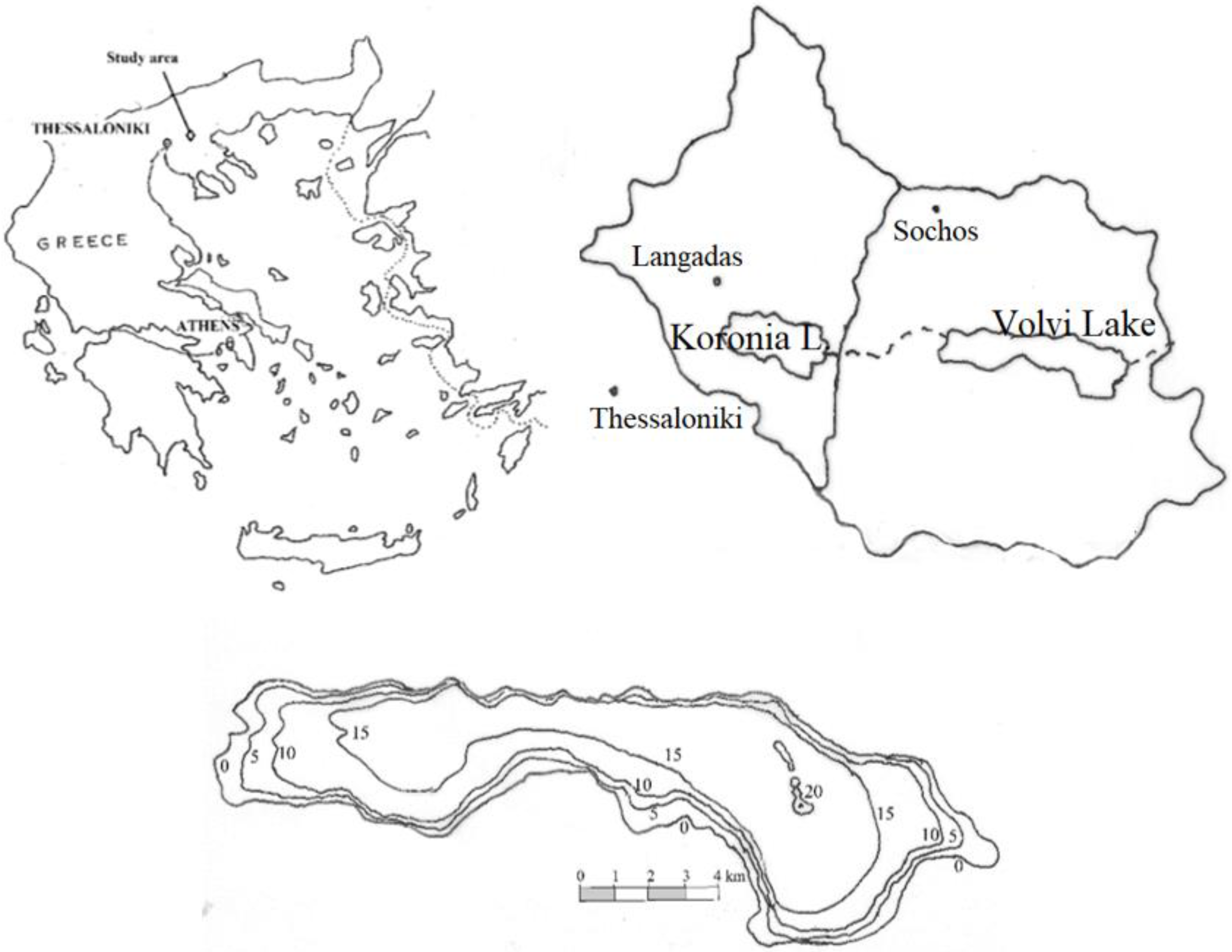
2.1. Site Description

Lake Volvi, along with Lake Koronia, is located in northern Greece and occupies the deeper part of the hydrological basin of Mygdonia (40°37’ N, 23°21’ E) at an altitude of 37 m above sea level (in 2012). Lake Koronia overflowed into Lake Volvi through a ditch until the 1990s. Lake Volvi overflows into the Strymonikos gulf through the Richios stream. The surface elevation, volume, surface area, and maximum depth of the lake in 2014 were 37.0 m above sea level, 1000 × 106 m3, 75.0 km2, and 23.5 m, respectively. The trophic status of the lake is considered oligotrophic to mesotrophic.
The lakes have a combined hydrological basin of a total area of 2024 km2, with the Lake Volvi subbasin occupying 1247 km2. Figure 1 shows the site in Greece, the hydrological basin, with the two subbasins of lakes Volvi and Koronia and the bathymetric map of Lake Volvi.
The lakes Volvi and Koronia are considered and protected by the Ramsar Convention as a system of water bodies of international importance for the value of the wetland habitat, ideal for a variety of flora and fauna species [38].

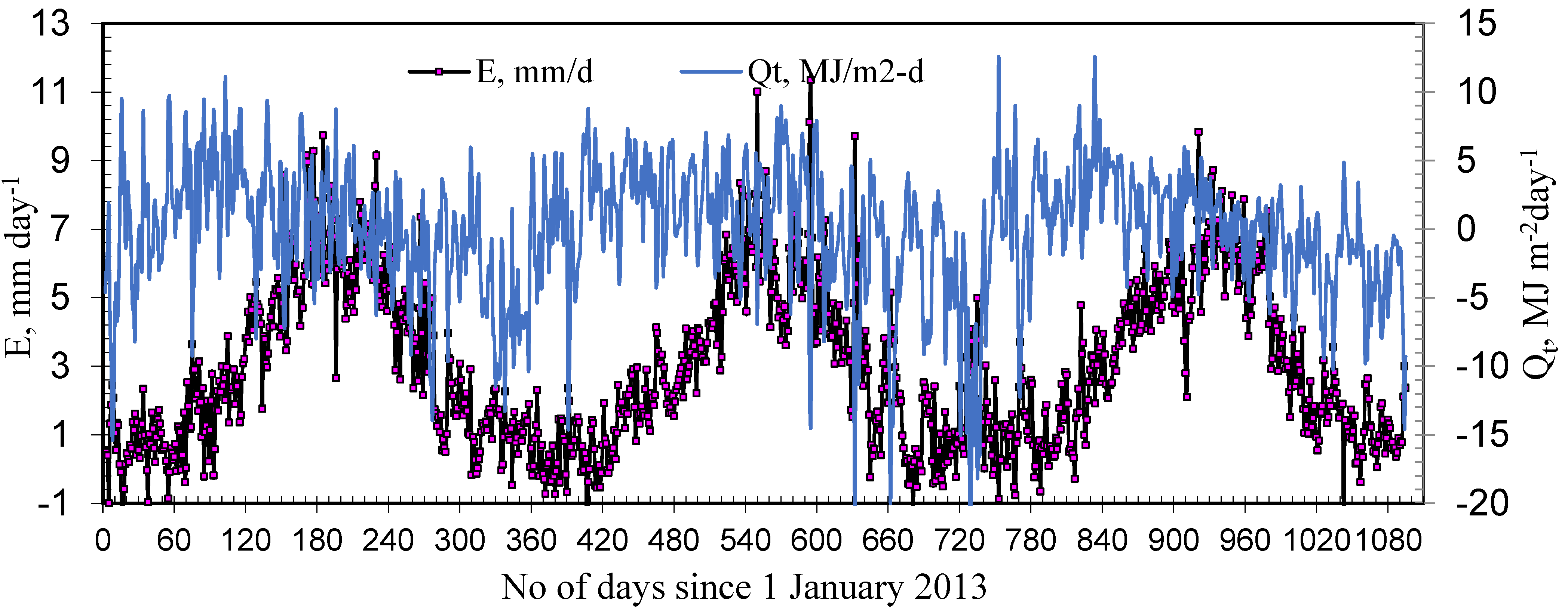
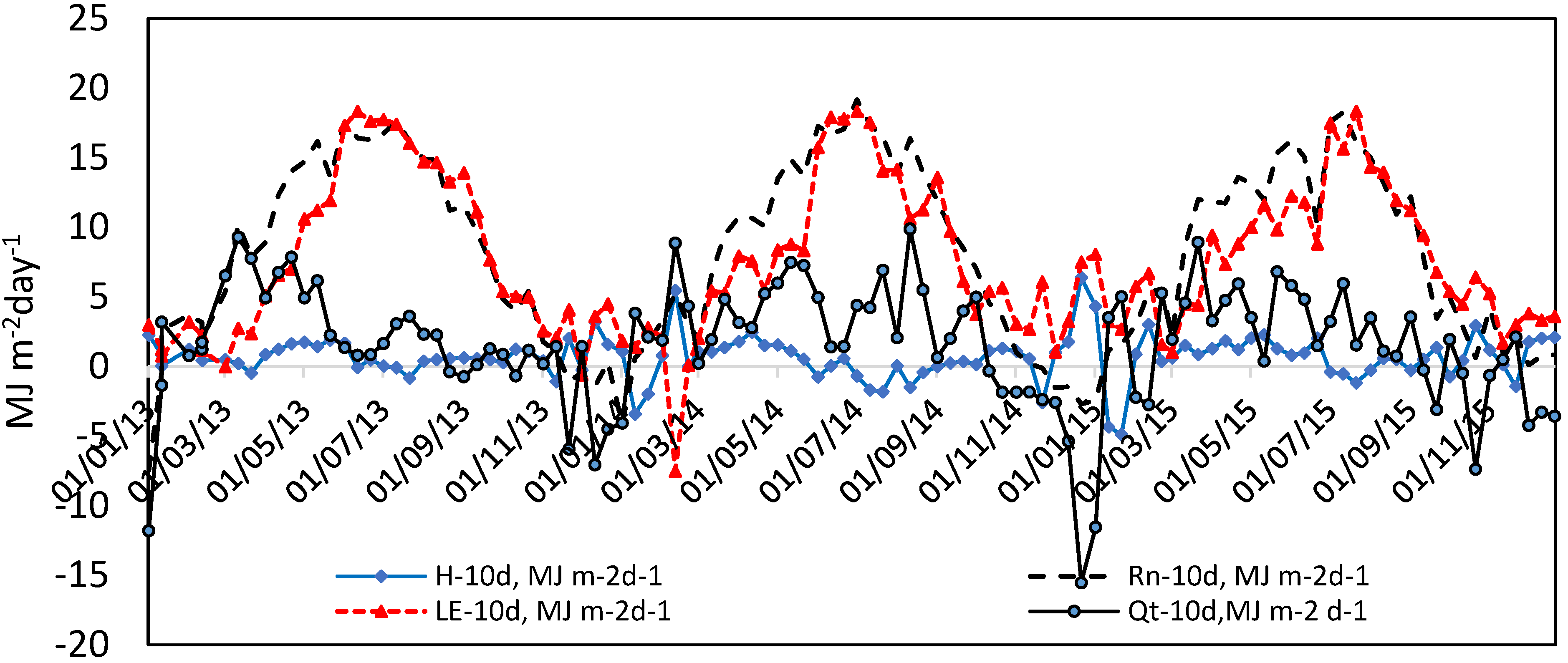
2.2. Water Surface Energy Budget

The water surface energy budget [32,39,40] is described by:
Qt = Rn − H − LE
where Qt is the change in the energy (thermal) content of the water body (MJ m−2 day−1), Rn is the net radiation (MJ m−2 day−1), H is the energy conducted to or from the body of water as sensible heat (MJ m−2 day−1), and LE is the latent heat flux (due to evaporation) (MJ m−2 day−1).
The net radiation (Rn) is described as:
R n = R s R s r + R a R a r R b r = ( 1 α s ) R s + ( 1 α a ) ε a σ ( T a + 273 ) 4 ε σ ( T s + 273 ) 4
where Rs and Ra are the short-wave radiation incident to water surface and the incoming long-wave radiation from the atmosphere, respectively (MJ m−2 day−1); Rsr and Rar are the reflected short-wave and long-wave radiation, respectively (MJ m−2 day−1); Rbr is the back (long-wave) radiation emitted from the body of water (MJ m−2 day−1); Ta is the air temperature above the water surface (°C); Ts is the surface water temperature (°C); αs is the reflectivity of the sort-wave radiation of the water surface (αs = 0.07); αa is the reflectivity of the long-wave radiation of the water surface (αa = 0.03); εa and ε are the atmospheric and water emissivity, respectively; and σ is the Stefan–Boltzmann constant (σ = 4.89 × 10⁻⁹ MJ m−2 day−1 K−4).
The flux of sensible heat (H) is related to the evaporative heat flux (LE) through the Bowen ratio (β) [41]:
β = H L E = γ T s T a e s w e d
where esw is the saturation vapor pressure at the temperature of the water surface (kPa), ed is the air vapor pressure above the water surface (kPa), and γ is the psychrometric constant (in kPa °C−1).
The change in the thermal content of the water body (Qt) is calculated using the change in the lake’s temperature for the time step [21,22], according to the equation:
Q t = ρ w c p w A s d d t 0 z m a x A T d z
in which cpw is the specific heat of water (ΜJ kg−1 °C−1), As is the surface area of the lake (m2), A(z) is the horizontal area as a function of depth (m2), and T(z,t) is the water temperature (°C) as a function of depth (z) and time (t).

2.3. Mathematical Modeling

The one-dimensional, eddy diffusion model QUALAKE has been used in the past [21,22] to study the water quality, evaporation and energy budget of Lake Vegoritis in Greece. The model uses the method of finite elements to solve the differential equations which describe the spatial and temporal changes of temperature and concentrations of phytoplankton (as the concentration of chlorophyll-α), soluble reactive phosphorus (SRP), organic phosphorus (OP) and dissolved oxygen (DO). The model was calibrated and verified using measured data of water quality parameters for different years [20,21,22]. The model results, during calibration and recalibration, showed that there was good agreement between simulated and measured values of the examined parameters [22].
The description of equations for the simulation of temperature, Chlα, phosphorus and DO distributions in the lake have been presented elsewhere [21,22]. In the following paragraphs, the equations for the submodels for water temperature, SRP, OP, primary production (expressed as the production of phytoplankton biomass) and dissolved oxygen are presented.

2.3.1. Lake Water Temperature Modeling

The heat transport is based on the one-dimensional vertical diffusion equation of the form [7,41,42]:
T t = 1 A z ( K A T z ) 1 A ( A q ) / z ρ w c p w
where K is the eddy diffusion coefficient (m2 day−1), q(z) is the internal distribution of heat sources due to solar radiation absorption inside the water column (MJ m−2 day−1), ρw is the water density (kg m−3), cpw is the specific heat of water (MJ kg−1 °C−1), A(z) is the horizontal area as a function of depth (m2), and T(z,t) is the water temperature (°C).
The internal distribution of solar radiation q(z) is given by [4]:
q ( z ) = ( 1 β s ) q s n exp ( η z )
where η is the extinction coefficient for solar radiation in water (m−1) and βs is the fraction of net short-wave radiation absorbed at the surface of the lake.
The eddy diffusion coefficient (K) is calculated using the following equation [20,43]:
K = K 0 f
where K0 is a reference value of K (m2 day−1), and f is a function of the Richardson number. The Richardson number depends on the vertical gradient of water temperature, the friction velocity (w*) and the coefficient of expansion. The value of K0 is related to the friction velocity, which is a function of wind velocity [41,44]. Details of the parameter f as a function of the Richardson number are given in Sundaram and Rehm (1973) [43] and Henderson-Sellers (1984) [41].

2.3.2. Water Quality Parameters Modeling

The one-dimensional vertical diffusion of each of the water quality parameters (SRP, OP, Chlα and DO) is described by a diffusion equation of the following form [9,45,46]:
C k t = 1 A z ( A K D C C k z ) + S k
in which Ck is the concentration of the k water quality parameter k (Ck equals CSRP, COP, CChlα, CDO, respectively) (mg m−3) as a function of depth (z, in m) and time (t, in days); A is the horizontal area of the lake at the depth z (m2); KDC is the vertical diffusion coefficient (m2 day−1); and Sk is a term describing the net production rate of the k parameter in each layer (mg m−3 day−1).
The diffusion coefficient of each water quality parameter is directly related to the vertical thermal stratification structure [46,47,48] and is usually identical to the thermal diffusivity coefficient, which is the sum of the coefficients of molecular diffusivity (Do, in m2 day−1) and turbulent diffusivity (E(z,t), in m2 day−1). It is estimated in each time step using a number of equations as presented by Antonopoulos and Gianniou (2003) [20].
The term Sk for the diffusion equation of SRP (k = SRP) includes the losses of SRP due to phytoplankton uptake and water outflows, as well as its sources from phytoplankton respiration, mineralization of organic phosphorus and water inflows in each layer, according to the equation:
S S R P = a p c P H + a p c R + M I N O P + 1 A Δ z ( Q i C S R P i Q 0 C S R P )
where apc is the phosphorus to chlorophyll-α concentration ratio in phytoplankton cells; PH is the phytoplankton growth rate (mg m−3 day−1); R is the phytoplankton respiration loss (mg m−3 day−1); Δz is the vertical spatial step (m); MINOP is the term describing the mineralization of OP to SRP (mg m−3 day−1); Qi and Q0 are the inflows and outflows of water from the lake, respectively (m3 day−1); and CSRPi and CSRP are the concentrations of SRP in inflow water and in the lake, respectively (mg m−3).
The term Sk for the diffusion equation of OP (k = OP) includes the losses of OP due to mineralization and the gains from the mortality of organisms in the lake, the water inflows and outflows and the losses due to sinking of OP:
S O P = a p c M M I N O P + 1 A Δ z ( Q i C O P i Q 0 C O P ) 1 A ( A w s O P C O P ) z
where M is the mortality rate of phytoplankton (mg Chlα m−3 day−1) including grazing by zooplankton, wsop is the sinking velocity of OP (m day−1), COPi is the concentration of OP in the inflowing water (mg m−3), and the other terms are already defined.
The term Sk for the diffusion equation of Chlα (k = Chlα) includes phytoplankton production by photosynthesis and the losses of phytoplankton biomass due to respiration, mortality and zooplankton grazing and the sinking of Chlα to sediments:
S C h l a = P H R M G Z 1 A ( A w s C h l a C C h l a ) z
where GZ is the loss due to zooplankton grazing (mg m−3 day−1) and wsChlα is the vertical velocity of phytoplankton sedimentation (sinking velocity) (m day−1).
The term Sk for the diffusion equation of DO (k = DO) includes oxygen production by photosynthesis and the losses due to respiration and the biochemical oxygen demand:
S D O = α o c P H α o c R S B O D
where αoc is the oxygen to chlorophyll-α concentration ratio and SBOD is the loss of biochemical oxygen demand (mg m−3 day−1).
The boundary condition at the water surface (z = 0) for SRP, OP and Chlα diffusion equations is considered to be zero flux across the boundary [22,48], while the boundary condition for DO is considered to be flux type due to the reaeration processes [21,22].
The bottom boundary condition (z = b) for SRP is defined by a flux term due to the release of SRP from the bottom sediments [21,22], while the bottom boundary condition (z = b) for the DO equation is described by the oxygen flux to satisfy the sediment oxygen demand (SOD). The bottom boundary condition (z = b) for OP and Chlα is defined by an equation of zero flux along the boundary [48].

2.4. Results Evaluation

The quantitative evaluation of the model results is based on the statistical criteria of root mean square error (RMSE) and correlation coefficient (r2) between the measured and simulated values [49]. The optimum value of RMSE criteria is zero, while r2 is one.

2.5. Data for Simulations

The meteorological variables for the study area were measured at a station located at the north-west of the lake at a distance of 35 km (National Observatory of Athens, Weather station of Lagadas) at 40°42′ N, 23°06′ E with an elevation of 87 m. These measured data include the daily values of maximum, minimum and average air temperature (Tmax,Tmin, and Tave, respectively), relative humidity (RHav), wind velocity (u2) and precipitation (Pr).
The climate of the study area is considered as semi-arid Mediterranean. The mean annual precipitation ranges between 450 and 600 mm, with a mean annual rain depth of 519 mm. The mean annual temperature is 13.3 °C, with the maximum monthly temperature occurring in July and the minimum in January.
Table 1 presents the maximum, minimum, and average values of temperature (°C), relative humidity (%), wind speed (m s−1), solar radiation (MJ m−2 day−1) and rainfall for each year of simulation and the average values for the time period from 2013 to 2019.
In the absence of sunshine duration or solar radiation data, the multi-linear regression (MLR) equation of solar radiation to meteorological variables from the meteorological station of the Aristotle University of Thessaloniki (AUTH), which is located north-west at a distance of 42 km (40°54′ N; 23°06′ E), was used [50]. This multi-linear regression (MLR) equation uses the meteorological variables Tmax, Tmin, Tav, RHav, Ra, TD (=Tmax − Tmin) and u2, with the following forms:
R s = 11 . 0267 + 0 . 47768 R a + 0 . 83564 ( TD ) 2 . 2386 ( TD ) 1 / 2 0 . 16562 RH av
The coefficient of determination (r2) of the model was 0.846, based on the daily dataset for the years 2011–2013 from the AUTH station.
The annual water balance of Lake Volvi, estimated with the MIKE HYDRO model using historical data from the period 1970 to 2000 [51], consists of an average direct precipitation of 421 mm, evaporation of 729 mm, runoff of 282 mm, pumping from the lake of 9.33 mm, outflow to the aquifer of 8.8 mm, and inflow from the aquifer of 5.5 mm. The average water balance of Lake Volvi was estimated at −38.89 mm/year.
The trophic status and the water quality of Lake Volvi are mainly affected by agricultural runoff, animal husbandry effluents, untreated or semi-treated domestic effluents and industrial wastewaters, mainly from food, dairy and other industries [52], as well as from suspended stream sediments and eroded bank materials.
Physical, chemical and biological variables for Lake Volvi were randomly measured for some short periods [52,53,54,55].
The mean values of SRP, TP and Chlα in water samples collected just below the surface of the water, as presented by Kaiserli et al. (2002) [52], were 60, 145, and 7.6 mg m−3, respectively. Similar values of SRP, TP and DO were presented by Petaloti et al. (2004) [55].
In a report of the Hellenic Ministry of Rural Development and Foods [56], a comparison of mean values of DO, phosphorus and nitrogen concentrations measured near lake surface water and near the bottom during two periods (1999–2000 and 2010–2012) was presented. Table 2 shows the average values of these parameters.
More systematic measurements of temperature, dissolved oxygen and phytoplankton (as chlorophyll-α), and nutrient concentration were conducted under the National Water Monitoring Network program during the years 2011 to 2015 [37].
Thus, the calibration and recalibration of the model had to be based on the available data from 2013 to 2015. Simulations started on 1 January, when, based on measurements and meteorological data, the initial condition for water temperature was set at 9 °C. The initial condition for chlorophyll-α, SRP, OP and DO was defined from sporadic data from other years [56] and the fact that the lake is fully mixed during winter.
The values of the constants and coefficients in most simulations were based on a combination of the values given in the literature and on a sensitivity analysis. In this paper, the values taken from the literature were corrected during the calibration process [15,22,39,57,58,59,60,61,62,63].

3. Results and Discussion

The mathematical model QUALAKE was used to simulate the temperature and the concentrations of SRP, OP, Chlα, and DO in Lake Volvi on a daily basis for the years 2013 to 2015. Simulations were started on 1 January and continued in daily time steps until the end of each year.
In the following paragraphs the results of the temperature, DO, SRP, OP, and Chlα simulations will be presented and analyzed.
The calibration of QUALAKE was based on the available data from the years 2013 to 2015. During the calibration, by the method of trial and error, the model parameters were adjusted so that the simulated results of Tw, DO, SRP, OP and Chlα compared well with the measured values. The parameters that were used in the simulations are given in Table 3.

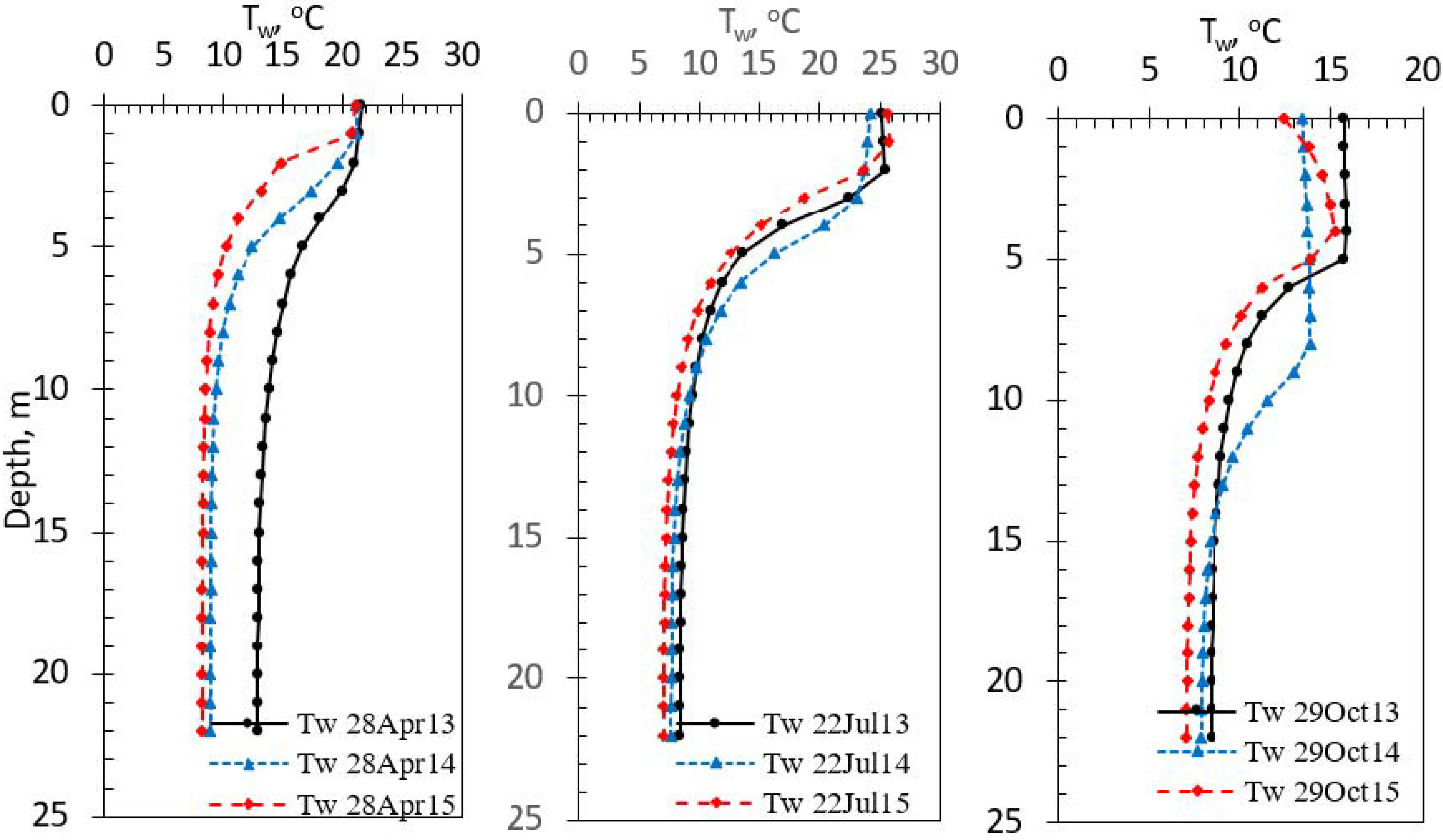
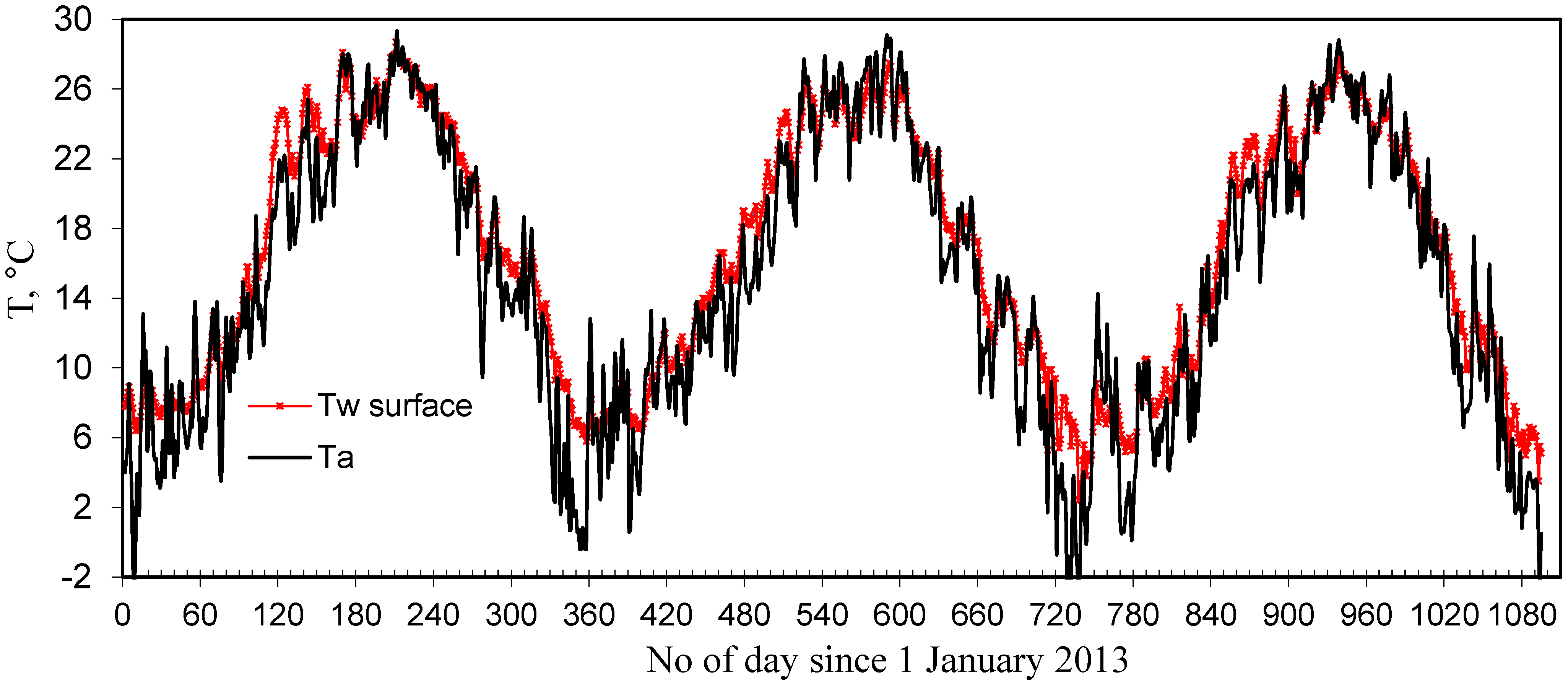
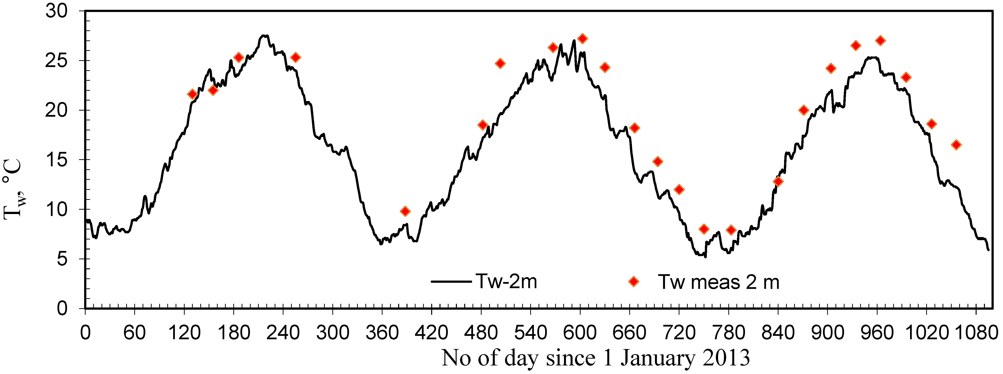
3.1. Water Temperature Simulation

In Figure 2, some characteristic simulated vertical lake water temperature profiles for specific days of the three years of the simulation are presented. Lake Volvi has the characteristic annual temperature cycle of temperate monomictic lakes. The model simulates well the onset of stratification, mixed layer depth and water temperature. In Figure 3, a comparison between simulated water surface temperature values and the air temperature is presented, while in Figure 4, a comparison of the simulated water temperature with the measurements at 2 m depth is presented.
The RMSE between the calculated and measured temperature values estimated for the available measurements of the three years of the simulation was 2.58 °C, while the coefficient of determination (r2) was 0.923. The RMSE value of temperature simulations for Lake Vegoritis (at a northern latitude of 40°47′) ranged from 0.42 to 1.84 °C [20]. The average RMSE and r2 values of the water temperature simulation in nine lakes of different morphological characteristics were 1.1 °C (ranging from 0.68 to 1.93 °C) and 0.92 (ranging from 0.89 to 0.95), respectively [64].
According to simulation results, the lake showed a characteristic annual temperature cycle. Temperature stratification was observed from the beginning of April, with a thermocline depth of 3 to 8 m. The depth of the thermocline increased during the summer and remained deep until October. Fall overturn occurred between the end of October and the beginning of November. The maximum depth of the thermocline reached 9 m. The thermocline depth increased faster and was deeper for the year 2014, maybe due to the higher values of the diffusion coefficient as a result of the higher wind velocity of this year.
The model evaluated evaporation and all energy budget components of Lake Volvi on a daily basis, as well as the daily distribution of lake water temperature with depth, the surface temperature (Tsw), and the change in the thermal content of the lake (Qt). The water temperature near the water–atmosphere interface of the lake controls the partitioning of available energy into latent and sensible heat [32]. An increased interest has developed in the water temperature and heat fluxes at the water–atmosphere interface during the last decades due to climate change. The results of energy budget and heat transport in the lakes, using models such as QUALAKE, could be considered reference data to develop different models based on artificial neural networks and energy budget models to estimate lake water surface temperature.
In Figure 5, the evaporation (E) values and thermal content change (Qt) during the three successive years of simulation are presented. The energy budget components of Lake Volvi for each year of the simulation and their average values are given in Table 4.
The average, maximum and minimum daily evaporation values are 3.03, 11.36 and −3.06 mm d−1, respectively, and the thermal content change values are −0.17, 12.59 and −23.34 MJ m−2 d−1, respectively. The average evaporation was higher in 2013 and lower in 2014. The mean evaporation rate estimated, with the QUALAKE model, for Lake Vegoritis was 2.59 mm day−1 [21].
Evaporation rates are low from the onset of calculations during winter and early spring. In summer, evaporation increases rapidly and remains high until early autumn. Negative evaporation rates (condensation) emerge during winter months.

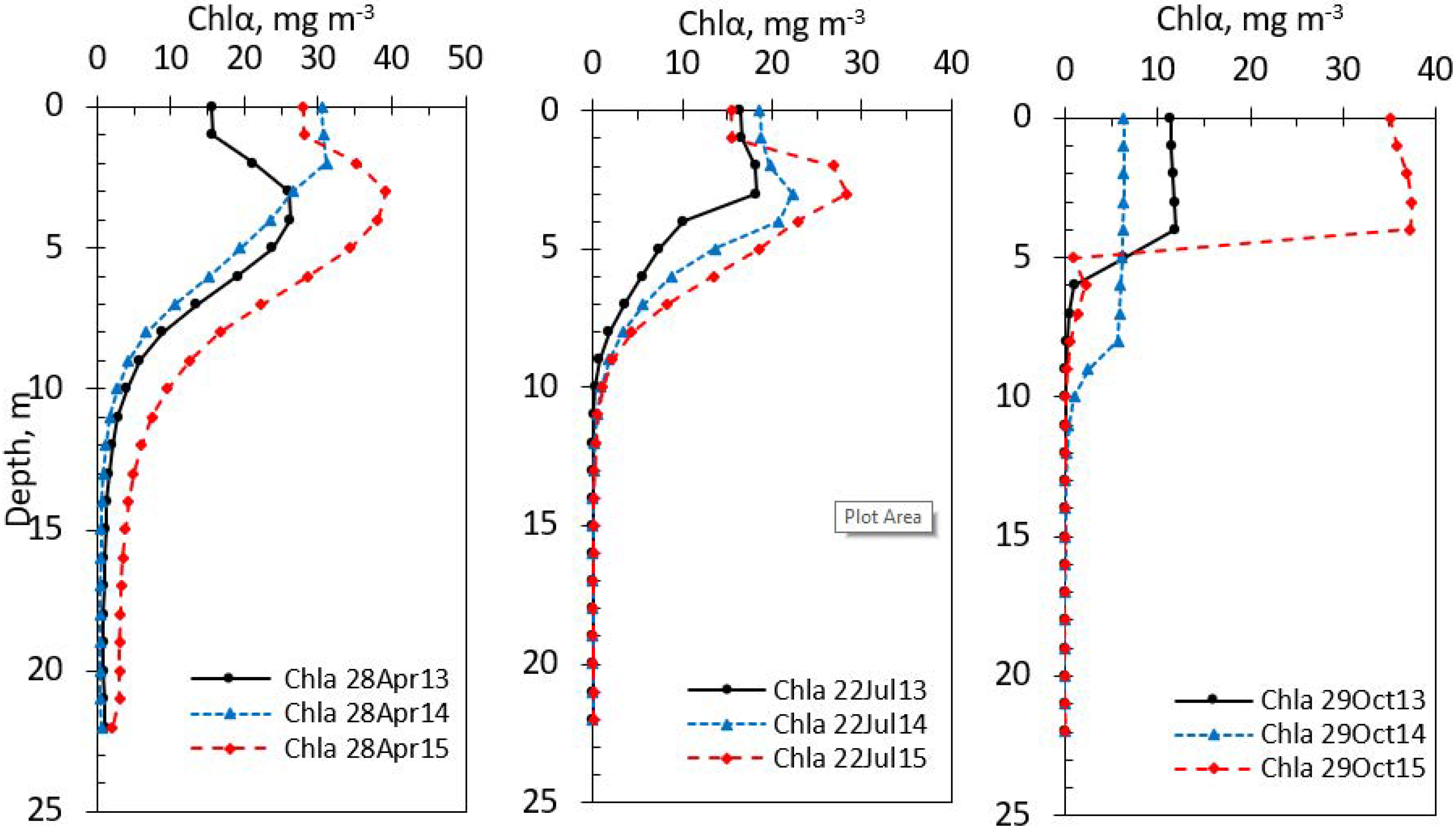
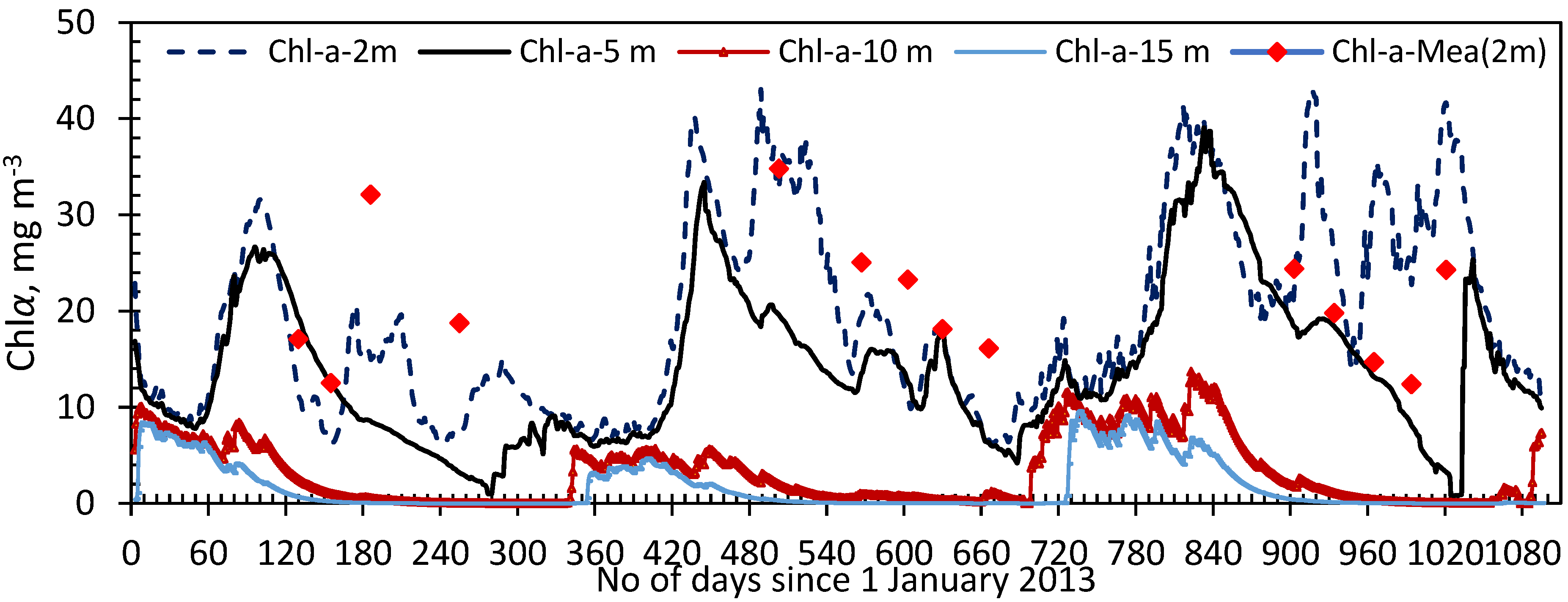
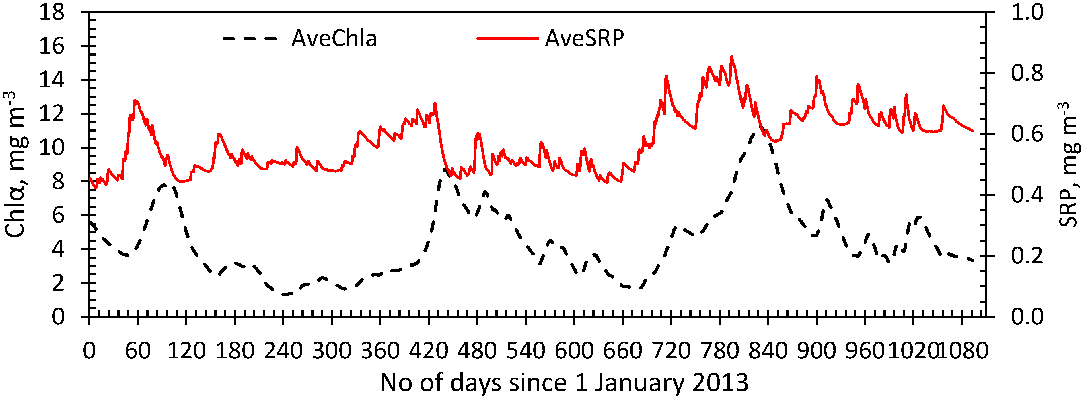
3.2. Phytoplankton in the Lake

In Figure 6, the simulated values of the chlorophyll-α concentration during the three successive years of the simulation are presented.
The annual variation of chlorophyll-α concentration at four different depths, along with the measured values at the 2 m depth, is presented in Figure 7. A comparison of the simulated results from the QUALAKE model against the measured values of chlorophyll-α at a depth of 2 m shows generally acceptable results. The variation of chlorophyll-α concentration in the epilimnion (depths 2 and 5 m) presents different patterns along the different years. The concentration at 2 m depth shows higher variation during the years 2014 and 2015. There are some small periods in the spring months of 2015 with peaks in concentration. The distribution at a depth of 5 m was smoother throughout the study period. The RMSE between the calculated and measured values of chlorophyll-α estimated for the available measured data of the three years of the simulation was 10.26 mg m−3.
During thermal stratification, there are intense differences in the vertical distribution of Chlα concentrations regarding the epilimnetic and hypolimnetic values, as well as the depth of the maximum epilimnetic values. This depth depends on the depth of the epilimnion and the euphotic zone and the circulation and stratification conditions of the lake. The concentrations in the hypolimnion (depths 10 and 15 m) were, as expected, significantly lower in comparison to the values in the epilimnion and were zero after April.
The average Chlα concentration during the three years of the simulation was 4.44 mg m−3, with a minimum annual average of 1.31 mg m−3 in 2013 and a maximum of 11.28 mg m−3 in 2015 (Table 5). In general, the Chlα concentrations were higher in 2015.

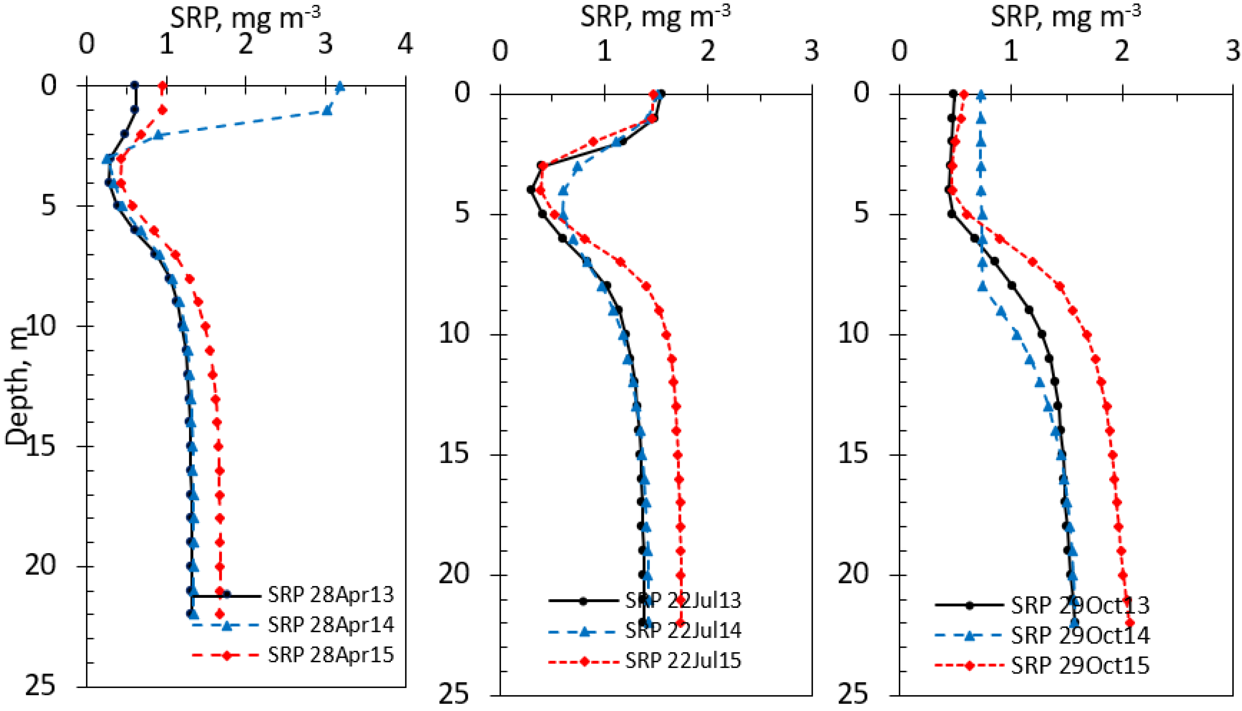
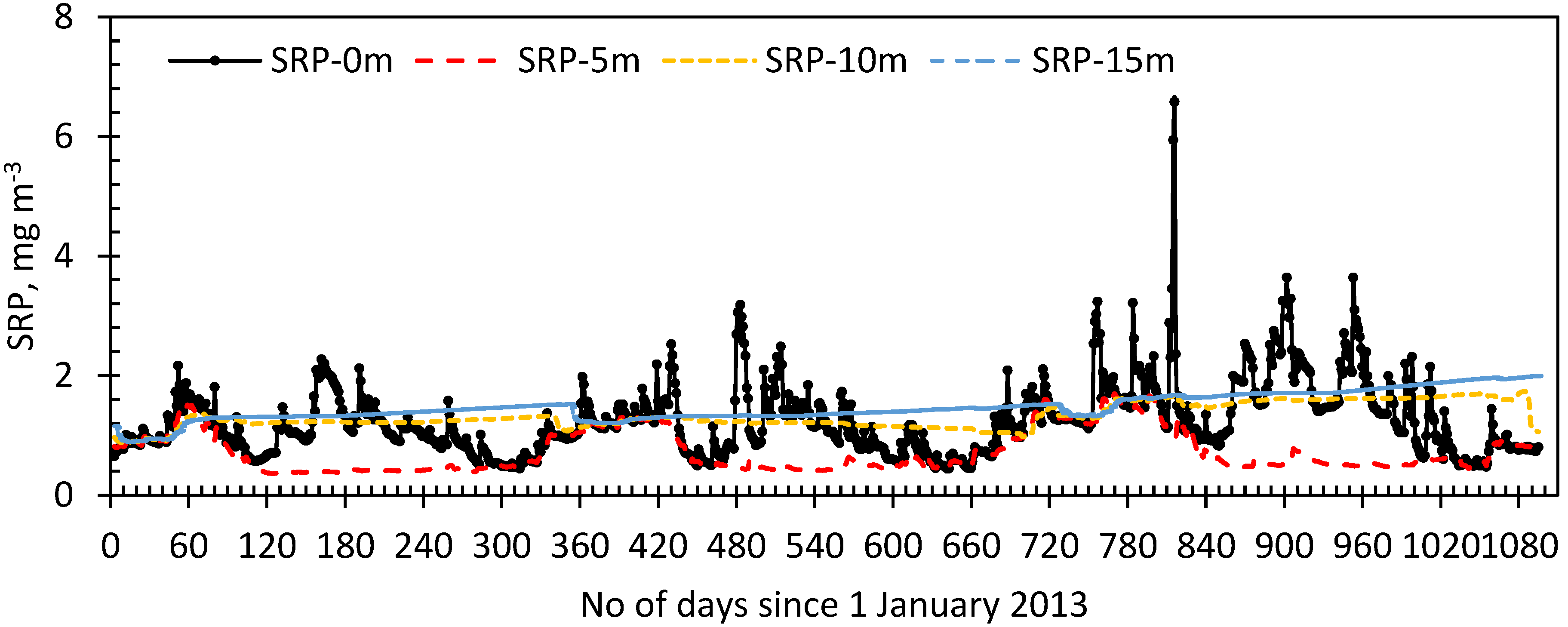
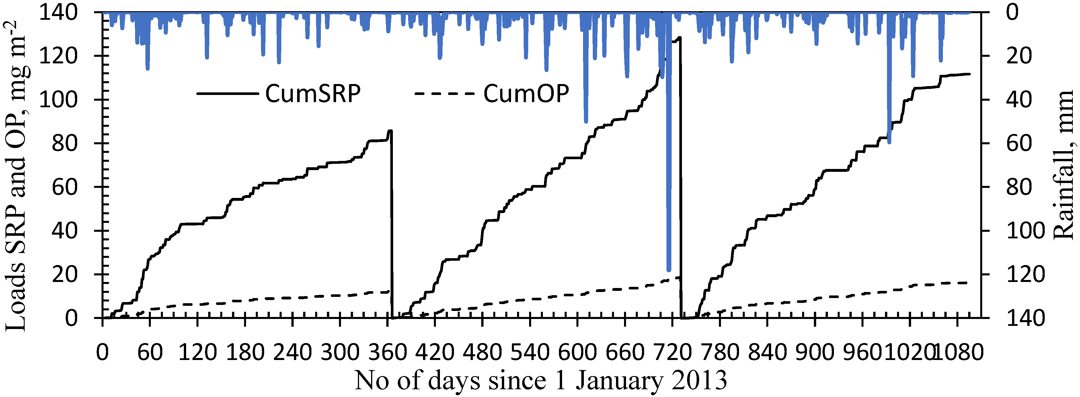
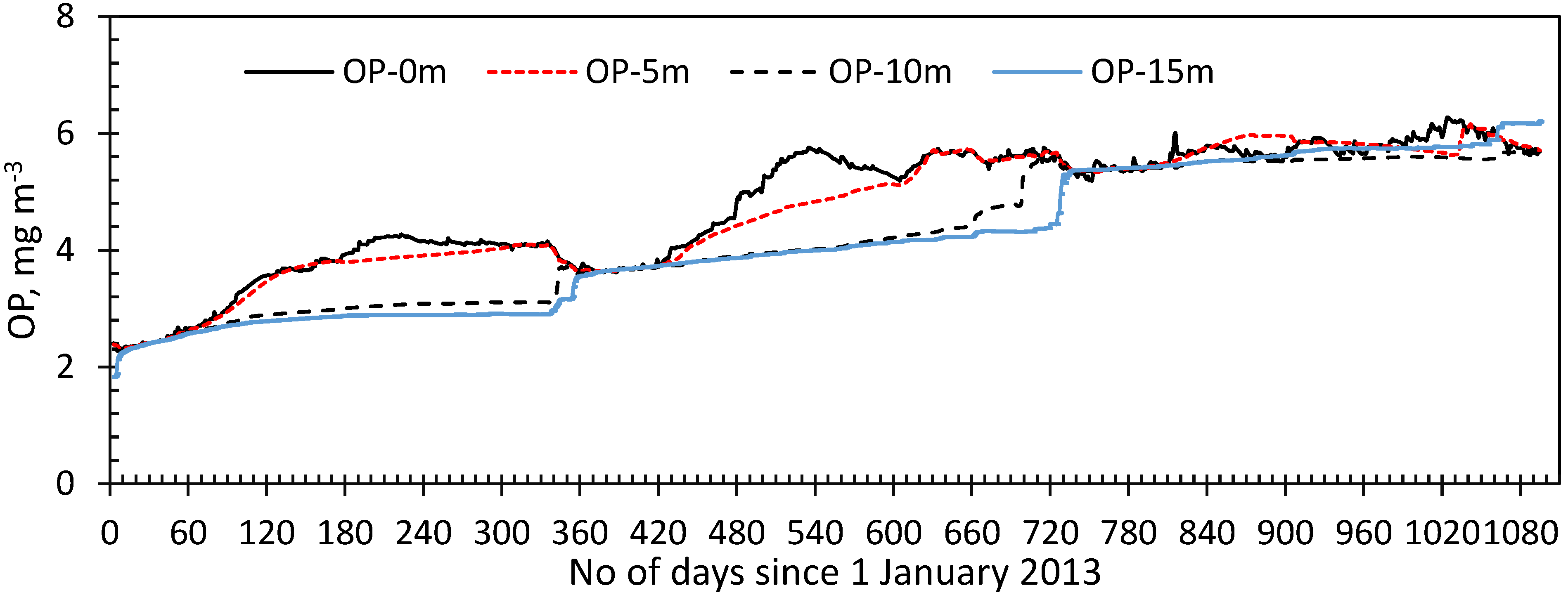
3.3. Phosphorus in the Lake

There are no measured data of phosphorus in Lake Volvi. Some measurements of total phosphorus concentration have been conducted on behalf of the Hellenic Ministry of Rural Development and Foods [56] and the National Water Monitoring Networks [37] for some specific years, but only in the surface layer of the lake.
A comparison of the SRP profiles simulated on different days of the three years is presented in Figure 8. In the spring, the distribution was similar under the thermocline depth, though very different in the surface layer. In the 3 to 8 m layer (metalimnetic layer), a decrease in concentration was observed during July, mainly due to the high phytoplankton production in this layer. Later in October, significantly lower surface concentrations were estimated in comparison to the previous months, as phytoplankton production remains high during this period of the year. The thermocline inhibits the mixing of the two layers (epilimnion and hypolimnion), and, therefore, SRP, which is produced in the hypolimnion by the mineralization of the sinking dead organic matter that accumulates there and continuously increases hypolimnetic SRP concentrations. In the deeper layers, the SRP concentrations for the years 2014 and 2015 were similar, although they were lower in 2013, mainly due to the lower concentrations of Chlα for this year.
The temporal distribution of SRP concentration during the three years is shown in Figure 9. Very intensive variation was observed at the surface, with high peaks in 2014 and especially in the first months of 2015. There were some periods in which the concentration of SRP was very high. These are connected to high rainfall and high runoff, which enriched the lake with inorganic phosphorus. Deeper in the hypolimnion, the calculated concentrations of SRP were relatively constant and, in general, lower than 2 mg m−3, although at different sizes during the different years of the simulation. In the 3 to 5 m depth layer near the thermocline, the SRP concentrations presented lower values in relation to the concentrations at other depths, as this is the layer where maximum phytoplankton growth takes place.
The cumulative daily loading of SRP in the lake for each year and the daily rainfall of the three-year period are presented in Figure 10. The total SPR loading of the three years was 85.65, 128.31 and 111.65 mg m−2, respectively, while the cumulative rainfall was 420.6, 914.7 and 573.6 mm, respectively.
The average SRP concentration in the lake during the three years of the simulation is presented in Figure 11. The mean value of the three years was 0.57 mg m−3, with a minimum average of 0.40 mg m−3 in 2013 and a maximum of 0.85 mg m−3 in 2014 (Table 5). A comparison of Chlα and SRP average concentrations (Figure 11) shows that there is an inverse correlation between the values of the two parameters.
The annual variation of OP concentrations at specific depths is presented in Figure 12. The concentration of OP in the epilimnion presented significant variation throughout the year. There is an increase in OP concentrations after February until the end of May, followed by a decrease with the lower values at the end of July. Then from September onward, an increase was again observed. The OP concentrations ranged from 2.3 to 4.2 mg m−3 in 2013, were higher in 2014 from 3.6 to 5.7 mg m−3, and from 5 to 6.3 mg m−3 in 2015 in the epilimnion and lower but continuously increased year to year in the hypolimnion (2.5 to 3.8 in 2013, 3.1 to 5.5 in 2014, and 5 to 6 mg m−3 in 2015).
Throughout the year, near-bottom OP concentrations were higher in relation to hypolimnetic concentrations. During the period of thermal stratification, OP is rapidly recycled in the epilimnion because of the high concentrations of phytoplankton and, as a result, zooplankton organisms. High OP values are observed in the bottom of the hypolimnion and the sediments, where the particulate portion of OP sinks and decomposes relatively slowly. The OP concentrations near the bottom throughout the year are higher in relation to hypolimnetic concentrations. The hypolimnetic OP concentrations were similar in 2013 and 2014, while they were notably higher in 2015, mainly due to the high phytoplankton growth rate and Chlα concentrations of this year.
The cumulative loading of OP to the lake is presented in Figure 10. The total OP loading for the three years of 2013–2015 was 12.36, 18.52 and 16.11 mg m−2, respectively.

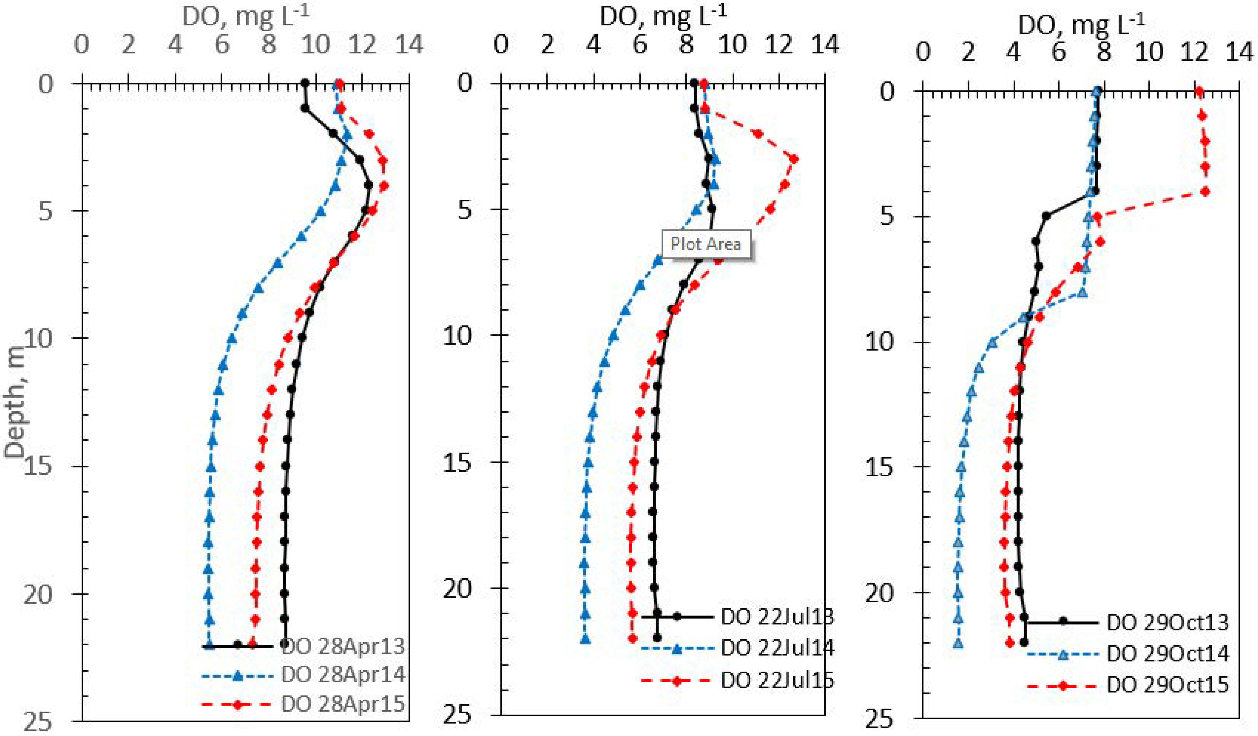
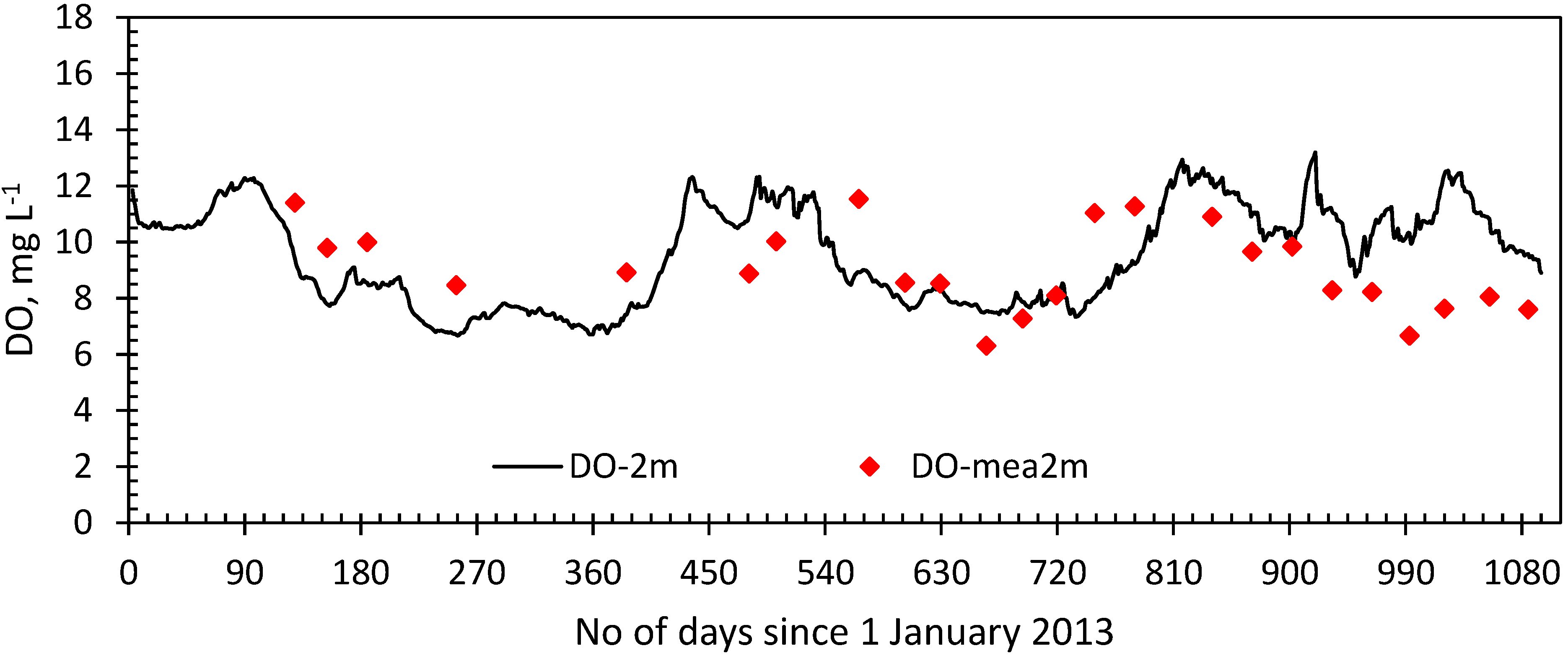
3.4. Dissolved Oxygen Simulation

In Figure 13, some characteristic simulated DO profiles are presented for specific days from the three years. DO concentration profiles during the first months of the year were nearly homogeneous, while during summer and early fall showed different distributions along the depth for each year of the simulation, following the patterns of the Chlα and temperature distributions. In the euphotic zone, the DO concentration decreased throughout each year. The DO values were less than 2 mg L−1 in the hypolimnion during the autumn of 2014, while the DO concentrations in 2013 and 2015 remained higher than 4 mg L−1. Due to stratification, the hypolimnion is cut off from the high epilimnetic oxygen concentrations. Non-occurrence of the metalimnetic oxygen minimum and the DO concentrations in the hypolimnion are evidence that lake Volvi is not under eutrophication pressure.
In Figure 14, the daily DO concentration at 2 m depth in comparison to the measurements taken during the three successive years is presented. The RMSE between the calculated and measured DO values estimated for the available measurements of the three years of the simulation was 2.085 mg L−1. The average RMSE values of DO in a number of lakes in the USA, presented by Stefan et al. (1993), were from 0.6 to 2.3 mg L−1 with an average of 1.4 mg L−1 [64].

3.5. Discussion

The evaluation of the model was based on measured data of temperature, DO and Chlα during three years from 2013 to 2015 in lake Volvi. This time period was selected as a result of the available data from the National Observatory of Athens in Greece [37]. Assessing the model based on the values of r2 and RMSE for these parameters, the performance of the QUALAKE model in Lake Volvi was quite good, especially when taking into consideration the uncertainties in model parameters and nutrient loading estimations and the absence of measurements of other water quality parameters. The values of the performance criteria are generally similar to those reported in other ecosystem model studies [10,64,65,66].
Parameters estimation is a critical point in the development of environmental models, according to Chapra (1997) [42]. The identification of parameter values is a very difficult task due to the inherent complexity of environmental systems, scarcity of data, and mathematical and computational limitations [67]. Saloranta and Andersen (2007) [8] noted that the performance of a model code is very much dependent on the particular task to which it is applied, implying that a general model code “validation” may be an unrealistic goal based on graphical estimates.
The energy budget for a lake relates to the net transfer of energy to and from the water. The temperature of the water and its variations express the changes in the stored thermal energy, and it is one of the principal water quality and quantity factors of lake hydro ecosystems. The changes in lake water temperature and the temperature stratification dynamics can have a profound effect on lake biological and chemical processes, as well as on their hydrological cycle.
Incoming (Ra) and outgoing (Rbr) long-wave radiation are the energy budget components with the largest mean annual rates (Ra = 28.49 MJ m−2 day−1 and Rbr = 33.51 MJ m−2 day−1). Because of their opposite signs, there is a mean loss of energy of 5.12 MJ m−2 day−1 (Table 4). Therefore, the source of energy is the net short-wave solar radiation (Rs) with a mean rate of 14.88 MJ m−2 day−1. Rs, Ra and Rbr radiation values exhibit a characteristic seasonal variation, with the highest rates in summer and the lowest in winter. Similarly, net radiation (Rn) obtains its largest values in the summer and its lowest in the winter, with a three-year average value of 7.97 MJ m−2 day−1. Its mean annual value is explicitly positive, as net radiation is the source of energy for all the physical and biological activities of the lake ecosystem.
The seasonal variation of the thermal content of the water body (Qt) is balanced between its positive and negative values of incoming and outgoing radiation and sensible and latent heat (Figure 15). In spring, the lake consecutively gains and stores thermal energy through net radiation. In summer, the energy budget is positive. In autumn and winter, the energy budget is negative since the stored energy is released as sensible and mainly as latent heat, resulting in the gradual cooling of the lake. For the three years of simulation, the total energy gain of Lake Volvi was −0.17 MJ m−2 day−1.
The average SRP concentrations were low for all years. SRP is rapidly used for phytoplankton growth in the euphotic zone due to the high primary productivity of the lake. The sinking dead organic matter accumulates in the hypolimnion, and its mineralization increases SRP concentrations in this layer, which cannot be transferred to the epilimnion because of the thermocline. The different meteorological conditions, with higher rainfalls at the end of 2014 and the beginning of 2015, had an important effect on inorganic phosphorus loads, increasing the SRP concentration in the lake and consequently increasing the photosynthesis rate. The latter also affected the DO concentrations in the epilimnion during the same period.
The average annual OP concentrations in the hypolimnion ranged from 2.8–5.4 mg m−3 during the three years. Similar, but slightly higher, were the values of OP in the epilimnion, which ranged from 3.6 to 5.7 mg m−3. The distribution with depth of OP values was nearly the same for all the years of the simulation, with only higher near the bottom values during 2015. A specific portion of OP sinks into the hypolimnion and the sediments, where it decomposes relatively slowly.
The Chlα concentration differed from year to year in regard to both magnitude and pattern (Figure 7). The maximum average Chlα concentration in the lake ranged from 7.79 mg m−3 (2013) to 10 mg m−3 (2015). The peaks in the Chlα concentration appeared from mid-spring to mid-summer, while in 2015, three peaks were observed (spring, summer, and autumn), which is characteristic of lakes that are becoming more productive [68]. The average Chlα concentration agrees with the WFD’s (the EU Water Framework Directive) water quality requirements for good ecological quality (Chlα concentration of deep-water lakes should not exceed 12 mg m−3).
The main environmental variables affecting primary productivity are nutrient availability, temperature, and solar radiation. As phosphorus is considered the limiting nutrient for phytoplankton growth in most lakes, phytoplankton concentrations are usually closely related to SRP concentrations. Comparing the distribution of SRP and Chlα from Figure 7, Figure 9 and Figure 11, the results show that phytoplankton concentrations throughout the year are strongly affected by SRP concentrations and vice versa [22]. Thus, high primary productivity at the end of winter and early spring causes concentrations of SRP to decrease rapidly during spring, followed by a reduction in phytoplankton production rates. During summer, a temporary recovery in SRP is observed as a result of a higher rate of mineralization due to the presence of dense populations of zooplankton organisms, which accelerate the process of mineralization. Huang et al. (2012) [69] considered that the chlorophyll-α concentration was highly sensitive to parameters directly related to growth rates (such as maximum phytoplankton growth rate and temperature, nutrient, and light factors).
The model results of the DO simulation showed that there was good agreement between the simulated and measured values of DO for the available data at a 2 m depth in the lake. According to measurements from the Hellenic Ministry of Rural Development and Foods [56], the mean values of DO concentrations measured near the lake water surface ranged from 8.2 to 9.8 during 1999–2000 and 8.5 to 10.4 during 2010–2012, and near the bottom of the lake from 6.0 to 6.4 during 1999–2000 and 2.1 to 5.1 during 2010–2012 (Table 2). Figure 14 and Figure 15 showed a similar distribution of DO in Lake Volvi.
Suitable calibrated and verified models for energy and water quality of lake ecosystems are necessary for lake water and ecosystem management. A lake’s ecosystem responds directly to climate change. Increasing water temperature affects the hydrodynamics in lakes, expanding the thermal stratification period and the depth of the thermocline [65,70,71]. Water temperature, the most sensitive parameter to climate change, is a key parameter in most biological reactions, influencing water chemistry, biochemical reactions, and aquatic organisms directly.
The results of energy and water quality parameters estimated for Lake Volvi for the three years of simulation showed that the model could be used for the management of the water quality of the lake. It can also be used to forecast the changes and effects in the status of the lake under climate change scenarios. The model should be recalibrated with more recent measured data either from the National Water Monitoring Network or more intensive measurements in the lake.

4. Conclusions

The one-dimensional mathematical model QUALAKE was used to describe energy (temperature, heat balance and evaporation), water quality (dissolved oxygen, inorganic and organic phosphorus) and biological productivity (phytoplankton–chlorophyll-α) during the annual cycle in a stratified lake and the results were presented and evaluated. The model simultaneously describes water temperature and concentrations of DO, SRP, OP, and phytoplankton (as chlorophyll-α) in a daily time step. It simultaneously calculates evaporation rates and energy budget components.
Data from Lake Volvi in Central Macedonia of Greece (in northern Greece) for three successive years (2013 to 2015) were used to calibrate and recalibrate the model.
The simulation results of the model’s application are an important source of information on changes in the physical, chemical and biological variables of the lake for which very few data are available. The energy, nutrients, and biological submodels were parameterized using literature data and verified by computing simulations of temperature, DO and Chlα patterns with field data.
The model results of water temperature, dissolved oxygen and chlorophyll-α were compared to measurements at 2 m depth for the years 2013 to 2015. The comparison showed that the predicted values of these parameters were all in good agreement with the measurements.
The results of the model simulations during the three successive years for energy, water quality and primary productivity showed that the average concentration of the studied parameters was 0.58 mg m−3 for SRP, 4.5 mg m−3 for OP, and 4.4 mg m−3 for Chlα. The DO in the epilimnion was near saturation, while in the hypolimnion remained higher than 2 mg L−1. The average evaporation from the water surface was 3.05 mm day−1.
There is a general deficiency in water quality modeling in Greece, mainly due to the lack of appropriate data for the application and validation of such models. This is the first time that a mathematical model, such as the QUALAKE model, has been applied to Lake Volvi, one of the most important impoundments in northern Greece, protected by the Ramsar International Convention. Furthermore, according to the EU Water Framework Directive 2000/60, Annex II 1.5, EU member states: “shall carry out an assessment of the likelihood that surface water bodies within the river basin district will fail to meet the environmental quality objectives set for the bodies under Article 4. Member states may utilize modeling techniques to assist in such an assessment”. The QUALAKE model could be used in fulfilling the Directive requirements, regarding Lake Volvi, in view of the scarcity of water quality data for this lake and the fact that a management plan for the river basin district of Lake Volvi has not yet been elaborated.

Author Contributions

Conceptualization, methodology, software, validation, formal analysis, investigation, resources, data curation, V.Z.A. and S.K.G.; writing—original draft preparation, V.Z.A.; writing—review and editing, visualization, V.Z.A. and S.K.G.; supervision, V.Z.A. All authors have read and agreed to the published version of the manuscript.

Funding

This research received no external funding.

Institutional Review Board Statement

Not applicable.

Informed Consent Statement

Informed consent was obtained from all subjects involved in the study.

Data Availability Statement

Data are available from the corresponding author upon request and subject to the Human Subjects protocol restrictions.

Acknowledgments

The authors would like to thank the (1) National Water Network of Hellenic Ministry of Environment and Energy, (2) Greek Biotope/Wetland Centre (EKBY), and (3) National Observatory of Athens, General Secretariat of Research and Innovation in Greece for providing the meteorological station datasets and water quality data.

Conflicts of Interest

The authors declare no conflict of interest.

References

  1. Chou, Q.; Nielsen, A.; Andersen, T.K.; Hu, F.; Chen, W.; Levi Ni, T.C.; Søndergaard, M.; Johansson, L.S.; Jeppesen, E.; Trolle, D. The impacts of extreme climate on summer-stratified temperate lakes: Lake Søholm, Denmark, as an example. Hydrobiologia 2021, 848, 3521–3537. [Google Scholar] [CrossRef]
  2. Kumar, A.; Mishra, S.; Bakshi, S.; Upadhyay, P.; Kumar-Thakur, T. Response of eutrophication and water quality drivers on greenhouse gas emissions in lakes of China: A critical analysis. Ecohydrology 2022, 16, e2483. [Google Scholar] [CrossRef]
  3. Malyan, S.K.; Singh, O.; Kumar, A.; Anand, G.; Singh, R.; Singh, S.; Yu, Z.; Kumar, J.; Fagodiya, R.K.; Kumar, A. Greenhouse Gases Trade-Off from Ponds: An Overview of Emission Process and Their Driving Factors. Water 2022, 14, 970. [Google Scholar] [CrossRef]
  4. Dake, J.M.K.; Harleman, D.R.F. Thermal stratification in Lakes-Analytical and Laboratory studies. Water Resour. Res. 1969, 5, 484–495. [Google Scholar] [CrossRef]
  5. Babajimopoulos, C.; Papadopoulos, F. Mathematical prediction of thermal stratification of Lake Ostrovo (Vegoritis), Greece. Water Resour. Res. 1986, 22, 1590–1596. [Google Scholar] [CrossRef]
  6. Hostetler, S.W.; Bartlein, P.J. Simulation of lake evaporation with application to modeling lake level variations of Harney-Malheur lake, Oregon. Water Resour. Res. 1990, 26, 2603–2612. [Google Scholar]
  7. Polli, B.A.; Bleninger, T. Reservoir 1D heat transport model. J. Applied Water Eng. Res. 2019, 7, 156–171. [Google Scholar] [CrossRef]
  8. Saloranta, T.M.; Andersen, T. MyLake—A multi-year lake simulation model code suitable for uncertainty and sensitivity analysis simulations. Ecol. Model. 2007, 207, 45–60. [Google Scholar] [CrossRef]
  9. Bonnet, M.-P.; Poulin, M. DyLEM-1D: A 1D physical and biochemical model for planktonic succession, nutrients and dissolved oxygen cycling. Application to a hyper-eutrophic reservoir. Ecol. Model. 2004, 180, 317–344. [Google Scholar] [CrossRef]
  10. Arhonditsis, G.B.; Brett, M.T. Eutrophication model for Lake Washington (USA) Part I. Model description and sensitivity analysis. Ecol. Model. 2005, 187, 140–178. [Google Scholar] [CrossRef]
  11. Wool, T.; Ambrose, R.; Martin, J.; Comer, E. Draft: User’s Manual for Water Quality Analysis Simulation Program (WASP)—Version 6.0; USEPA: Atlanta, GA, USA, 2002. [Google Scholar]
  12. Hipsey, M.R.; Romero, J.R.; Antenucci, J.P.; Hamilton, D.P. The Computational Aquatic Ecosystem Dynamics Model (CAEDYM): v3.2 Science Manual; Technical Report; Centre for Water Research University of Western Australia: Perth, Australia, 2006. [Google Scholar]
  13. Gal, G.; Imberger, J.; Zohary, T.; Antenucci, J.; Anis, A.; Rosenberg, T. Simulating the thermal dynamics of Lake Kinneret. Ecol. Model. 2003, 162, 69–86. [Google Scholar] [CrossRef]
  14. Hamilton, D.; Schladow, D. Prediction of water quality in lakes and reservoirs. Part I—Model description. Ecol. Model. 1997, 96, 91–110. [Google Scholar] [CrossRef]
  15. Cole, T.M.; Wells, S.A. CE-QUAL-W2: A Two-Dimensional, Laterally Averaged, Hydrodynamic and Water Quality Model, Version 3.0.; Technical Report; US Army Engineering and Research Development Center: Vicksburgh, MS, USA, 2000. [Google Scholar]
  16. U.S. Army Corps of Engineers (USACE). CE-QUAL-R1: A Numerical One Dimensional Model of Reservoir Water Quality. User’s Manual; Instruction Report E-82–1; U.S. Army Corps of Engineers Waterways Experiment Station: Vicksburg, MS, USA, 1995. [Google Scholar]
  17. Mi, C.; Shatwell, T.; Ma, J.; Wentzky, V.-C.; Boehrer, B.; Xu, Y.; Rinke, K. The formation of a metalimnetic oxygen minimum exemplifies how ecosystem dynamics shape biogeochemical processes: A modelling study. Water Res. 2020, 175, 115701. [Google Scholar] [CrossRef]
  18. Edlund, M.B.; Almendinger, J.E.; Fang, X.; Ramstack Hobbs, J.M.; Vander Meulen, D.D.; Key, R.L.; Engstrom, D.R. Effects of Climate Change on Lake Thermal Structure and Biotic Response in Northern Wilderness Lakes. Water 2017, 9, 678. [Google Scholar] [CrossRef] [Green Version]
  19. Xu, R.; Pang, Y.; Hu, Z.; Hu, X. The Spatiotemporal Characteristics of Water Quality and Main Controlling Factors of Algal Blooms in Tai Lake, China. Sustainability 2022, 14, 5710. [Google Scholar] [CrossRef]
  20. Antonopoulos, V.Z.; Gianniou, S.K. Simulation of water temperature and dissolved oxygen distribution in Lake Vegoritis, Greece. Ecol. Model. 2003, 160, 39–53. [Google Scholar] [CrossRef]
  21. Gianniou, S.K.; Antonopoulos, V.Z. Evaporation and energy budget in Lake Vegoritis, Greece. J. Hydrol. 2007, 345, 212–223. [Google Scholar] [CrossRef]
  22. Gianniou, S.K.; Antonopoulos, V.Z. Primary production and phosphorus modeling in Lake Vegoritis, Greece. Adv. Oceano. Limnol. 2014, 5, 18–40. [Google Scholar] [CrossRef]
  23. Andreadakis, A.; Noutsopoulos, C.; Gavalaki, E. Assessment of the water quality of lake Plastira through mathematical modelling for alternative management scenarios. Glob. Nest Int. J. 2003, 5, 99–105. [Google Scholar]
  24. Gikas, G.D.; Yiannakopoulou, T.; Tsihrintzis, V.A. Water quality trends in a lagoon impacted by non-point source pollution after implementation of protective measures. Hydrobiologia 2006, 563, 385–406. [Google Scholar] [CrossRef]
  25. Markou, D.A.; Sylaios, G.K.; Tsihrintzis, V.A.; Gikas, G.D.; Haralambidou, K. Water quality of Vistonis lagoon, Northern Greece: Seasonal variation and impact of bottom sediments. Desalination 2007, 210, 83–97. [Google Scholar] [CrossRef]
  26. Petriki, O.; Zervas, D.; Doulgeris, C.; Bobori, D. Assessing the Ecological Water Level: The Case of Four Mediterranean Lakes. Water 2020, 12, 2977. [Google Scholar] [CrossRef]
  27. Skoulikidis, N.; Kaberi, H.; Sakellariou, D. Patterns, origin and possible effects of sediment pollution in a Mediterranean lake. Hydrobiologia 2008, 613, 71–83. [Google Scholar] [CrossRef]
  28. Mellios, N.; Kofinas, D.; Laspidou, C.; Papadimitriou, T. Mathematical modeling of trophic state and nutrient flows of lake Karla using the PCLake model. Environ. Process. 2015, 2, S85–S100. [Google Scholar] [CrossRef] [Green Version]
  29. Doulgeris, C.; Georgiou, P.; Papadimos, D.; Papamichail, D. Ecosystem approach to water resources management using the MIKE 1 modeling system in the Strymonas River and Lake Kerkini. J. Environ. Manag. 2012, 94, 132–143. [Google Scholar] [CrossRef]
  30. Antonopoulos, V.Z.; Gianniou, S.K.; Antonopoulos, A.V. Artificial neural networks and empirical equations to estimate daily evaporation: Application to Lake Vegoritis, Greece. Hydrol. Sci. J. 2016, 61, 2590–2599. [Google Scholar] [CrossRef] [Green Version]
  31. Zhang, J.; Zhao, L.; Deng, S.; Xu, W.; Zhang, Y. A critical review of the models used to estimate solar radiation. Renew. Sustain. Energy Rev. 2017, 70, 314–329. [Google Scholar] [CrossRef]
  32. Antonopoulos, V.Z.; Gianniou, S.K. Analysis and Modelling of Temperature at the Water—Atmosphere Interface of a Lake by Energy Budget and ANNs Models. Environ. Processes 2022, 9, 15. [Google Scholar] [CrossRef]
  33. Heddam, S.; Ptak, M.; Zhu, S. Modelling of daily lake surface water temperature from air temperature: Extremely randomized trees (ERT) versus Air2Water, MARS, M5Tree, RF and MLPNN. J. Hydrol. 2020, 588, 125130. [Google Scholar] [CrossRef]
  34. Li, X.; Sha, J.; Wang, Z.-L. Chlorophyll-a prediction of lakes with different water quality patterns in China based on hybrid neural networks. Water 2017, 9, 524. [Google Scholar] [CrossRef] [Green Version]
  35. Zhu, W.-D.; Qian, C.-Y.; He, N.-Y.; Kong, Y.-X.; Zou, Z.-Y.; Li, Y.-W. Research on Chlorophyll-a Concentration Retrieval Based on BP Neural Network Model—Case Study of Dianshan Lake, China. Sustainability 2022, 14, 8894. [Google Scholar] [CrossRef]
  36. Alexandridis, T.K.; Takavakoglou, V.; Crisman, T.L.; Zalidis, G.C. Remote Sensing and GIS Techniques for Selecting a Sustainable Scenario for Lake Koronia, Greece. Environ. Manag. 2007, 39, 278–290. [Google Scholar] [CrossRef]
  37. HM-EE. Project Results on Water Monitoring Network; Hellenic Ministry of Environment and Energy: Athens, Greece, 2015. [Google Scholar]
  38. Ramsar Convention Bureau. Criteria for Identifying Wetlands of International Importance. Annexes to Recommendation 4.2, Montreaux, Switzerland, 1990, and Resolution V1–2, Brisbane, Australia, 1996; Ramsar Convention Bureau: Gland, Switzerland, 1996. [Google Scholar]
  39. Bowie, G.; Mills, W.; Porcella, D.; Campbell, C.; Pagenkopf, J.; Rupp, G.; Johnson, K.; Chan, P.; Gherini, S. Rates, constants and kinetics formulations in surface water quality modelling. EPA 1985, 600, 3–85. [Google Scholar]
  40. Sturrock, A.; Winter, T.; Rosenberry, D. Energy budget evaporation from Williams Lake: A closed lake in north central Minnesota. Water Resour. Res. 1992, 28, 1605–1617. [Google Scholar] [CrossRef]
  41. Henderson-Sellers, B. Engineering Limnology; Pitman Publishing: London, UK, 1984. [Google Scholar]
  42. Chapra, S. Surface Water-Quality Modeling; McGraw-Hill: New York, NY, USA, 1997. [Google Scholar]
  43. Sundaram, T.R.; Rehm, R.G. The seasonal thermal structure of deep temperate lakes. Tellus 1973, 25, 157–168. [Google Scholar] [CrossRef]
  44. Hutchinson, G.A. Treatise on Limnology. Geography, Physics and Chemistry; Wiley: New York, NY, USA, 1975; Volume 1. [Google Scholar]
  45. Omlin, M.; Reichert, P.; Forster, R. Biogeochemical model of Lake Zürich: Model equations and results. Ecol. Model. 2001, 141, 77–103. [Google Scholar] [CrossRef]
  46. Riley, M.; Stefan, H. MINLAKE: A dynamic lake water quality simulation model. Ecol. Model. 1988, 43, 155–182. [Google Scholar] [CrossRef]
  47. Chen, C.; Ji, R.; Schwab, D.; Beletsky, D.; Fahnenstiel, G.; Jiang, M.; Johengen, T.; Vanderploeg, H.; Eadie, B.; Wells Budd, J.; et al. A model study of the coupled biological and physical dynamics in Lake Michigan. Ecol. Model. 2002, 152, 145–168. [Google Scholar] [CrossRef] [Green Version]
  48. Walters, R. A time-and depth-dependent model for physical, chemical and biological cycles in temperate lakes. Ecol. Model. 1980, 8, 79–96. [Google Scholar] [CrossRef]
  49. Loague, K.; Green, R.E. Statistical and graphical methods for evaluating solute transport models: Overview and application. J. Contam. Hydrol. 1991, 7, 51–73. [Google Scholar] [CrossRef]
  50. Antonopoulos, V.Z.; Papamichail, D.M.; Aschonitis, V.G.; Antonopoulos, A.V. Solar radiation estimation methods using ANN and empirical models. Comput. Electron. Agric. 2019, 160, 160–167. [Google Scholar] [CrossRef]
  51. Kolokytha, E.; Malamataris, D. Integrated Water Management Approach for Adaptation to Climate Change in Highly Water Stressed Basins. Water Resour. Manag. 2020, 34, 1173–1197. [Google Scholar] [CrossRef]
  52. Kaiserli, A.; Voutsa, D.; Samara, C. Phosphorus fractionation in lake sediments—Lakes Volvi and Koronia, N. Greece. Chemosphere 2002, 46, 1147–1155. [Google Scholar] [CrossRef] [PubMed]
  53. Gantidis, N.; Pervolarakis, M.; Fytianos, K. Assessment of the quality characteristics of two lakes (Koronia and Volvi) of N. Greece. Environ. Monit. Assess. 2007, 125, 175–181. [Google Scholar] [CrossRef]
  54. Kastridis, A.; Kamperidou, V. Influence of land use changes on alleviation of Volvi Lake wetland (North Greece). Soil Water Res. 2015, 10, 121–129. [Google Scholar] [CrossRef] [Green Version]
  55. Petaloti, C.; Voutsa, D.; Samara, C.; Sofoniou, M.; Stratis, I.; Kouimtzis, T. Nutrient Dynamics in Shallow Lakes of Northern Greece. Env. Sci Pollut Res. 2004, 11, 11–17. [Google Scholar] [CrossRef]
  56. HM-RDF. Chemical Water Quality Monitoring of Irrigation Water (Surface and Groundwater) at River Runoff Basins of Macedonia-Thrace and Thessalia Areas; Technical Report of Project Metro 125A1 of PAA 2007–2013; Hellenic Ministry of Rural Development and Foods: Athens, Greece, 2015. [Google Scholar]
  57. Di Toro, D.; Connolly, J. Mathematical models of water quality in large lakes. Part 2: Lake Erie. U.S. Environmental Protection Agency, Environmental Research Laboratory, Office of Research and Development, Minnesota. EPA 1980, 600, 231. [Google Scholar]
  58. Romero, J.; Antenucci, J.; Imberger, J. One- and three-dimensional biogeochemical simulations of two differing reservoirs. Ecol. Model. 2004, 174, 143–160. [Google Scholar] [CrossRef]
  59. Schladow, G.; Hamilton, D. Prediction of water quality in lakes and reservoirs: Part II—Model calibration, sensitivity analysis and application. Ecol. Model. 1997, 96, 111–123. [Google Scholar] [CrossRef]
  60. Stefan, H.; Fang, X. Dissolved oxygen model for regional lake analysis. Ecol. Model. 1994, 71, 37–68. [Google Scholar] [CrossRef]
  61. Stefan, H.G.; Fang, X.; Hondozo, M. Simulated climate chnage effects on year-round water temperatures in temperate lakes. Clim. Change 1998, 40, 547–576. [Google Scholar] [CrossRef]
  62. Thomann, R.; Mueller, J. Principles of Surface Water Quality Modeling and Control; Harper and Row Publishers: New York, NY, USA, 1987. [Google Scholar]
  63. Zhang, J.; Jørgensen, S.; Mahler, H. Examination of structurally dynamic eutrophication model. Ecol. Model. 2004, 173, 313–333. [Google Scholar] [CrossRef]
  64. Stefan, H.G.; Hondozo, M.; Fang, X. Lake water quality modeling for projected future climate scenarios. J. Enviro. Quality. 1993, 22, 417–431. [Google Scholar] [CrossRef]
  65. Arhonditsis, G.B.; Winder, M.; Brett, M.T.; Schindler, D.E. Patterns and mechanisms of phytoplankton variability in Lake Washington (USA). Water Res. 2004, 38, 4013–4027. [Google Scholar] [CrossRef]
  66. Trolle, D.; Skovgaard, H.; Jeppesen, E. The Water Framework Directive: Setting the phosphorus loading target for a deep lake in Denmark using the 1D lake ecosystem model DYRESM-CAEDYM. Ecol. Model. 2008, 219, 138–152. [Google Scholar] [CrossRef]
  67. McDonald, C.P.; Bennington, V.; Urban, N.R.; McKinley, G.A. 1-D test-bed calibration of a 3-D Lake Superior biochemical model. Ecol. Model. 2012, 225, 115–126. [Google Scholar] [CrossRef]
  68. Moustaka-Gouni, M.; Nikolaidis, G. Phytoplankton of a warm monomictic lake—Lake Vegoritis, Greece. Arch. Fur Hydrobiol. 1990, 199, 299–313. [Google Scholar] [CrossRef]
  69. Huang, J.; Gao, J.; Hormann, G. Hydrodynamic-phytoplankton model for short-term forecasts of phytoplankton in Lake Taihu, China. Limnologica 2012, 42, 7–18. [Google Scholar] [CrossRef]
  70. Antonopoulos, V.Z.; Gianniou, S.K. Lake Vegoritis in Greece: A Paradigm of Climate Change and Mismanagement Effects on Its Quantity and Quality Characteristics. In Proceedings of the EWRA 7th International Conference: Water Resources Conservancy and Risk Reduction Under Climatic Uncertainty, Limassol, Cyprus, 25–27 June 2009; pp. 273–280. [Google Scholar]
  71. Komatsu, E.; Fukushima, T.; Harasawa, H.A. Modeling approach to forecast the effect of long-term climate change on lake water quality. Ecol. Model. 2007, 209, 351–366. [Google Scholar] [CrossRef]
Figure 1. Hydrological basin of Lake Volvi with the two subbasins of lakes Volvi and Koronia and the bathymetric map of Lake Volvi.
Sustainability 15 02505 g001
Figure 2. Simulated temperature profiles in Lake Volvi from 2013 to 2015 at specific days.
Sustainability 15 02505 g002
Figure 3. Variation of simulated water surface temperature (Tw surface) and air temperature (Ta) for Lake Volvi from 2013 to 2015.
Sustainability 15 02505 g003
Figure 4. Comparison of simulated (Tw-2m) and measured (Tw meas 2 m) water temperature at 2 m depth of Lake Volvi from 2013 to 2015.
Sustainability 15 02505 g004
Figure 5. Daily evaporation (E) and thermal content change (Qt) in Lake Volvi from 2013 to 2015.
Sustainability 15 02505 g005
Figure 6. Simulated chlorophyll-α concentrations in Lake Volvi at specific days from the years 2013 to 2015.
Sustainability 15 02505 g006
Figure 7. Yearly variation of chlorophyll-α concentration in Lake Volvi from 2013 to 2015.
Sustainability 15 02505 g007
Figure 8. Simulated SRP concentrations in Lake Volvi at specific days from the years 2013 to 2015.
Sustainability 15 02505 g008
Figure 9. Yearly variation of SRP concentration at different depths (0, 5, 10 and 15 m) in Lake Volvi from 2013 to 2015.
Sustainability 15 02505 g009
Figure 10. Daily rainfall and cumulative loads of SRP (CumSRP) and OP (CumOP) for Lake Volvi from 2013 to 2015.
Sustainability 15 02505 g010
Figure 11. Average concentrations of SRP (AveSRP) and Chlα (AveChla) in Lake Volvi from 2013 to 2015.
Sustainability 15 02505 g011
Figure 12. Annual variation of OP concentration at different depths (0, 5, 10 and 15 m) in Lake Volvi from 2013 to 2015.
Sustainability 15 02505 g012
Figure 13. Simulated dissolved oxygen profiles in Lake Volvi at specific days from the years 2013 to 2015.
Sustainability 15 02505 g013
Figure 14. Comparison of simulated (DO-2m) and measured (DO-mea2m) dissolved oxygen at 2 m depth of Lake Volvi from 2013 to 2015.
Sustainability 15 02505 g014
Figure 15. Annual variation of net radiation (Rn), sensible (H) and latent (LE) heat, and thermal content of the water body (Qt) for Lake Volvi from 2013 to 2015 (values in 10-day averages).
Sustainability 15 02505 g015
Table 1. Basic metrological data for the three years of simulation and for the time period from 2013 to 2019.
Tave, °CRHave, %Rainfall, mmu2,
m s−1
Rs, MJ m−2day−1
2013Ave15.4875.5420.600.62415.04
Max29.39725.82.64128.37
Min−2.54400.0000.76
2014Ave15.6875.5914.700.82714.08
Max29.1971183.42029.19
Min−2.54400.0000.01
2015Ave14.3771.5573.600.46315.29
Max28.89859.64.22227.2
Min−4.14700.0000.31
2013–2019Ave15.0171.77539.330.37215.54
Max30.4981024.73.68330.02
Min−8.339.5396.60.0000.01
Table 2. Average values of some water quality parameters for the periods of 1999–2000 and 2010–2012.
1999–20002010–20121999–20002010–2012
Surface WaterBottom Water
DO, mg L−18.2 to 9.88.5 to 10.46.0 to 6.42.1 to 5.1
P2O5, mg L−10.15 to 0.190.13 to 0.150.19 to 0.290.08 to 0.15
Inor N, mg L−10.10 to 0.980.11 to 0.390.170.49
Table 3. Values of constants and coefficients used in the simulation.
SymbolConstants and Coefficients ValueUnitsEquation
βsfraction of net short-wave radiation absorbed at the water surface0.35 (8)
ηextinction coefficient for solar radiation0.601/m(8)
σ constant in relation to turbulent diffusion coefficient and Richardson number0.012 (8)
nconstant as σ0.95 (9)
c2constant in relation to reference value of turbulent
diffusion coefficient and friction velocity
0.08 (9)
Phosphorus
apcphosphorus to chlorophyll-α concentration ratio0.5mg P mg−1 Chlα((11),(12))
kminmineralization constant0.01–0.02day−1((11),(12))
kmchlMichaelis–Menten constant for the mineralization of OP25.0mg Chlα m−3((11),(12))
kSDprelease rate of SRP from the sediments0.5mg SP m−2 day−1
KDOSDMichaelis–Menten constant for the release of SRP from the sediments in relation to the DO concentration0.05g DO m−3
wsopvertical velocity of organic phosphorus sedimentation0.005m day−1(12)
Phytoplankton
PHmaxmaximum growth rate of phytoplankton 1.5day−1((11),(13))
qoptoptimal light intensity level2.95MJ m−2 day−1((11),(13))
KpMichaelis–Menten constants for phosphorus4mg P m−3((11),(13))
krcoefficient of respiration loss of phytoplankton0.07day−1((11),(13))
kmtotcoefficient of mortality loss (including grazing) of
phytoplankton
0.05day−1(13)
wsvertical velocity of phytoplankton sedimentation
(sinking velocity)
0.005m day−1(13)
Table 4. Energy budget components (in MJ m−2d−1) of Lake Volvi for the three years of simulation (2013 to 2015).
RsRaRbrLEHQtE,
mm day−1
2013Ave15.1128.6433.827.530.79−0.323.07
Max28.3936.1139.3923.906.0511.119.73
Min2.6212.2728.70−3.23−10.17−17.54−1.31
2014Ave14.2628.9433.627.160.530.032.92
Max29.2035.6038.7527.889.548.7911.36
Min1.8621.1528.49−7.51−8.02−23.34−3.06
2015Ave15.2627.8833.107.600.76−0.213.10
Max27.2235.1738.8824.157.4912.599.84
Min2.5519.1027.31−5.13−8.71−17.99−2.09
2013–2015Ave14.8828.4933.517.430.69−0.173.03
Max29.2036.1139.3927.889.5412.5911.36
Min1.8612.2727.31−7.51−10.17−23.34−3.06
Notation: Rs is the short-wave radiation; Ra is the long-wave radiation from the atmosphere; Rbr is the back (long-wave) radiation; Qt is the change in the energy content of the water body; H is the sensible heat; LE is the latent heat flux; and E is the evaporation (mm day−1).
Table 5. Average, minimum and maximum values of water quality parameters in water surface and at 2 m depth and the average with depth values of SRP and Chlα from 2013 to 2015.
Ta, °COP
(0 m), mg m−3
SRP
(0 m),
mg m−3
Chlα
(0 m),
mg m−3
Tw (2m), °CDO (2 m), mg L−1Average
SRP,
mg m−3
Average
Chlα,
mg m−3
Ave201315.483.591.0512.3616.768.900.523.39
Max201329.304.272.2731.4627.5112.290.717.86
Min2013−2.50 2.320.445.856.476.670.421.31
Ave201415.685.011.1317.9616.449.120.544.22
Max201429.105.753.1840.8227.0412.320.798.70
Min2014−2.503.620.446.156.746.750.441.63
Ave201514.245.721.5321.9214.7510.570.675.71
Max201528.806.276.5842.4125.3413.180.8611.28
Min2015−4.105.190.478.675.207.340.573.16
ave2013–201515.134.771.2317.4115.999.530.584.44
max2013–201529.306.276.5842.4127.5113.180.8611.28
min2013–2015−4.102.320.445.855.206.670.421.31
Disclaimer/Publisher’s Note: The statements, opinions and data contained in all publications are solely those of the individual author(s) and contributor(s) and not of MDPI and/or the editor(s). MDPI and/or the editor(s) disclaim responsibility for any injury to people or property resulting from any ideas, methods, instructions or products referred to in the content.

