
Investigation of Predictive Regulation Strategy of Secondary Loop in District Heating Systems
 ,
,
Abstract
:1. Introduction
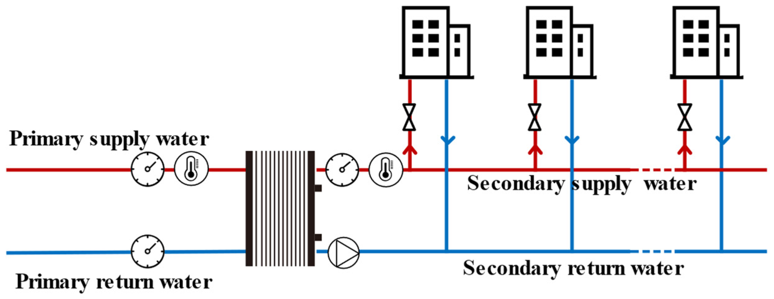
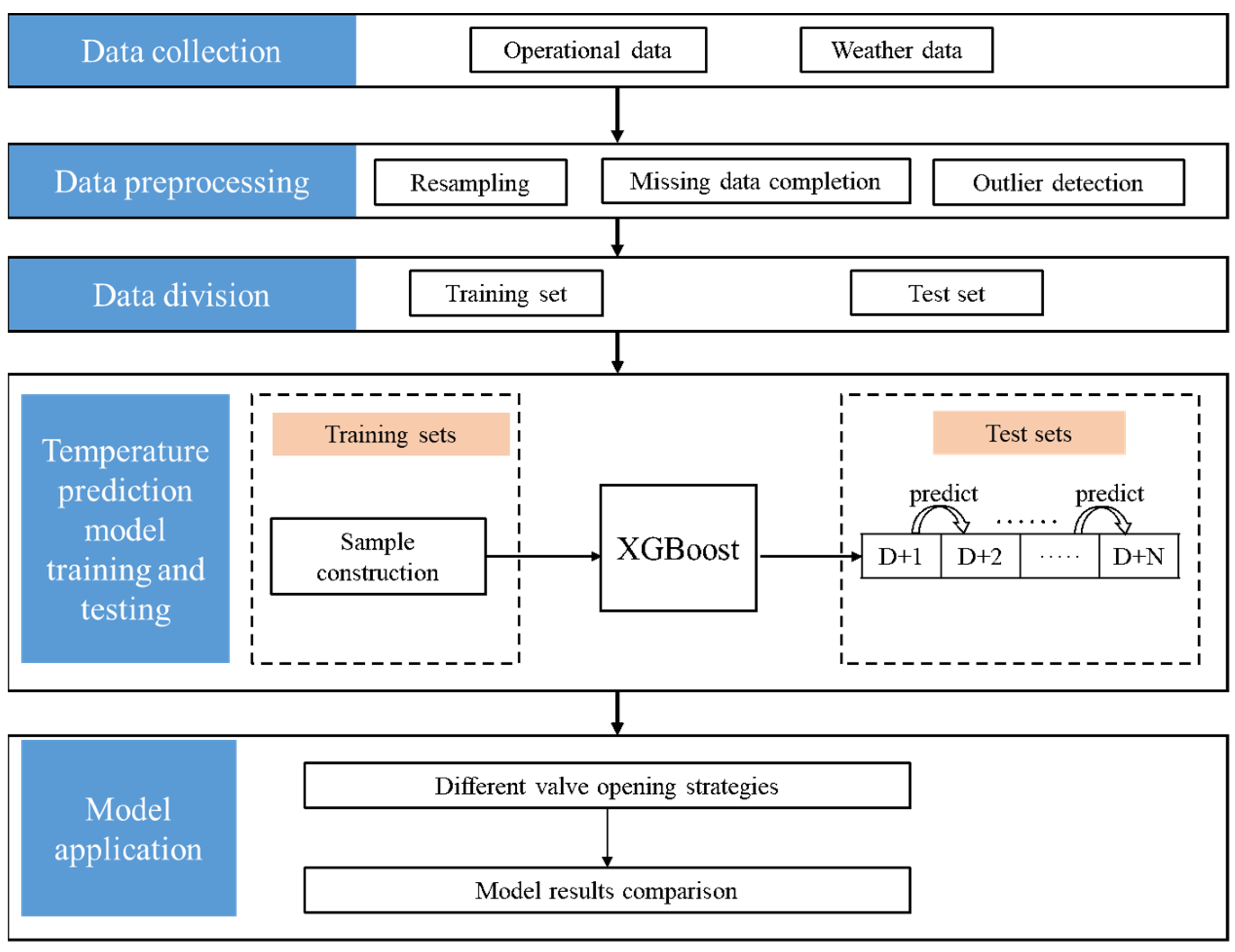
2. Methodology
- Remove repeating data:
- 2.
- Complete data and down-sampling:
- 3.
- Detect and replace outliers:
XGBOOST
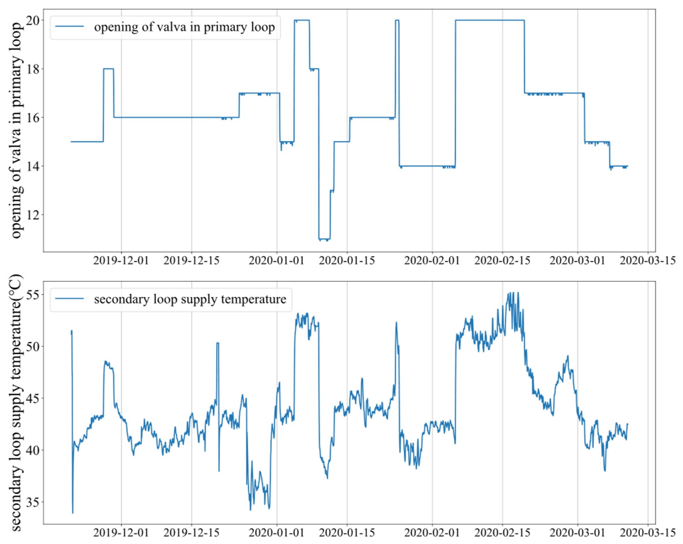
3. Results and Discussion
4. Conclusions
- The prediction performance of the machine learning model is compared under different input step sizes and prediction step sizes. The XGBoost model with 72 steps of input and 24 steps of prediction is used as the temperature response prediction model, the average prediction error of which is 0.26%, which has a high prediction accuracy;
- The XGBoost model with 72 steps of input and 24 steps of prediction is used to compare different valve opening control strategies. Based on the model, the valve control strategy of the heating substation is determined, which can realize the predictive control of the heating substation, improve the control accuracy of the heating substation, and reduce the dependence on manual experience;
- The work of this paper was practically applied in a real district heating system in Zhengzhou, China. The final validation results showed that the adoption of the proposed regulation strategy resulted in a 5% improvement in system energy efficiency.
Author Contributions
Funding
Institutional Review Board Statement
Informed Consent Statement
Data Availability Statement
Conflicts of Interest
References
- Zhong, W.; Huang, W.; Lin, X.; Li, Z.; Zhou, Y. Research on data-driven identification and prediction of heat response time of urban centralized heating system. Energy 2020, 212, 118742. [Google Scholar] [CrossRef]
- The Building Energy Conservation Research Center of Tsinghua University. Annual Research Report on the Development of Building Energy Efficiency in China 2019; China Architecture and Building Press: Beijing, China, 2019. [Google Scholar]
- Zheng, J.; Zhou, Z.; Zhao, J.; Wang, J. Effects of the operation regulation modes of district heating system on an integrated heat and power dispatch system for wind power integration. Appl. Energy 2018, 230, 1126–1139. [Google Scholar] [CrossRef]
- Wang, H.; Wang, H.; Zhu, T. A new hydraulic regulation method on district heating system with distributed variable-speed pumps. Energy Convers. Manag. 2017, 147, 174–189. [Google Scholar] [CrossRef]
- Stevanovic, V.D.; Zivkovic, B.; Prica, S.; Maslovaric, B.; Karamarkovic, V.; Trkulja, V. Prediction of thermal transients in district heating systems. Energy Convers. Manag. 2009, 50, 2167–2173. [Google Scholar] [CrossRef]
- Gu, J.; Wang, J.; Qi, C.; Yu, X.; Sundén, B. Analysis of a hybrid control scheme in the district heating system with distributed variable speed pumps. Sustain. Cities Soc. 2019, 48, 101591. [Google Scholar] [CrossRef]
- Gustafsson, J.; Delsing, J.; van Deventer, J. Experimental evaluation of radiator control based on primary supply temperature for district heating substations. Appl. Energy 2011, 88, 4945–4951. [Google Scholar] [CrossRef]
- Henze, G.P.; Floss, A.G. Evaluation of temperature degradation in hydraulic flow networks. Energy Build. 2011, 43, 1820–1828. [Google Scholar] [CrossRef]
- Mendes, N.; Oliveira, G.; Araújo, H. Building thermal performance analysis by using matlab/simulink. In Proceedings of the Seventh International IBPSA Conference, Rio de Janeiro, Brazil, 13–15 August 2001. [Google Scholar]
- Karlsson, J.; Wadsö, L.; Öberg, M. A conceptual model that simulates the influence of thermal inertia in building structures. Energy Build. 2013, 60, 146–151. [Google Scholar] [CrossRef]
- Yu, Z.; Haghighat, F.; Fung, B.C.M.; Yoshino, H. A decision tree method for building energy demand modeling. Energy Build. 2010, 42, 1637–1646. [Google Scholar] [CrossRef]
- Touzani, S.; Granderson, J.; Fernandes, S. Gradient boosting machine for modeling the energy consumption of commercial buildings. Energy Build. 2018, 158, 1533–1543. [Google Scholar] [CrossRef]
- Magnier, L.; Haghighat, F. Multiobjective optimization of building design using TRNSYS simulations, genetic algorithm, and Artificial Neural Network. Build. Environ. 2010, 45, 739–746. [Google Scholar] [CrossRef]
- Machado, J.E.; Cucuzzella, M.; Scherpen, J.M.A. Modeling and passivity properties of multi-producer district heating systems. Automatica 2022, 142, 110397. [Google Scholar] [CrossRef]
- Xu, B.; Huang, A.; Fu, L.; Di, H. Simulation and analysis on control effectiveness of TRVs in district heating systems. Energy Build. 2011, 43, 1169–1174. [Google Scholar] [CrossRef]
- Chicherin, S.; Anvari-Moghaddam, A. Adjusting heat demands using the operational data of district heating systems. Energy 2021, 235, 121368. [Google Scholar] [CrossRef]
- Wang, R.; Wang, Q.; Wei, C.; Cong, M.; Zhou, Z.; Ni, L.; Liu, J.; Wei, W. A Thermo-Hydraulic couplings model for residential heating system based on Demand-side Regulation: Development and calibration. Energy Build. 2022, 256, 111667. [Google Scholar] [CrossRef]
- Zheng, J.; Zhou, Z.; Zhao, J.; Hu, S.; Wang, J. Effects of intermittent heating on an integrated heat and power dispatch system for wind power integration and corresponding operation regulation. Appl. Energy 2021, 287, 116536. [Google Scholar] [CrossRef]
- Zhao, J.; Lyu, L.; Han, X. Operation regulation analysis of solar heating system with seasonal water pool heat storage. Sustain. Cities Soc. 2019, 47, 101455. [Google Scholar] [CrossRef]
- Sun, C.; Liu, Y.; Gao, X.; Wang, J.; Yang, L.; Qi, C. Research on control strategy integrated with characteristics of user’s energy-saving behavior of district heating system. Energy 2022, 245, 123214. [Google Scholar] [CrossRef]
- Wang, D.; Zhi, Y.-Q.; Jia, H.-J.; Hou, K.; Zhang, S.-X.; Du, W.; Wang, X.-D.; Fan, M.-H. Optimal scheduling strategy of district integrated heat and power system with wind power and multiple energy stations considering thermal inertia of buildings under different heating regulation modes. Appl. Energy 2019, 240, 341–358. [Google Scholar] [CrossRef]
- Cadau, N.; Lorenzi, A.D.; Gambarotta, A.; Morini, M.; Saletti, C. A Model-in-the-Loop application of a Predictive Controller to a District Heating system. Energy Procedia 2018, 148, 352–359. [Google Scholar] [CrossRef]
- Bojic, M.; Trifunovic, N. Linear programming optimization of heat distribution in a district-heating system by valve adjustments and substation retrofit. Build. Environ. 2000, 35, 151–159. [Google Scholar] [CrossRef]
- Turski, M.; Sekret, R. Buildings and a district heating network as thermal energy storages in the district heating system. Energy Build. 2018, 179, 49–56. [Google Scholar] [CrossRef]
- Ruseljuk, P.; Dedov, A.; Hlebnikov, A.; Lepiksaar, K.; Volkova, A. Comparison of District Heating Supply Options for Different CHP Configurations. Energies 2023, 16, 603. [Google Scholar] [CrossRef]
- García-Céspedes, J.; Herms, I.; Arnó, G.; de Felipe, J.J. Fifth-Generation District Heating and Cooling Networks Based on Shallow Geothermal Energy: A review and Possible Solutions for Mediterranean Europe. Energies 2023, 16, 147. [Google Scholar] [CrossRef]


| Modeling Scale | Research Target | Highlights | Ref. |
|---|---|---|---|
| DHS | thermal characteristic of DHS | Model the room air temperature and a multi-layer model for the building envelope | [10] |
| thermal characteristic of DHS | The effects of wall thickness, wall area, free solar radiation, and other factors on building heat storage were studied | [11] | |
| DHS | regulation of DHS | A building energy demand forecasting model based on the decision tree method | [12] |
| regulation of DHS | A baseline modeling based on the gradient boosting machine to forecast the energy consumption. | [13] | |
| thermal characteristic of DHS | Combine neural networks with multi-objective genetic algorithms for optimization studies of thermal comfort and energy consumption in buildings | [14] | |
| regulation of DHS | Address a comprehensive nonlinear ODE-based thermo-hydraulic model of the DHS | [15] | |
| thermal characteristic of DHS | Develop an integrated model for simulating the thermal and hydraulic behavior of the DHS | [16] | |
| thermal characteristic of DHS | Thermal inertia of buildings affects their behavior differently in terms of needed space heating | [17] | |
| regulation of DHS | A steady-state, bottom-up approach, and sequential linear programming was used to solve the unbalanced distribution of heat in a DHS | [25] | |
| regulation of DHS | The energetic effect of using buildings and a district heating network as thermal energy storage to compensate for the reduced heat output of the DHS | [26] | |
| Primary loop of DHS | regulation of DHS | Genetic algorithm is used to optimize the adjustment strategy of distributed variable speed pump in DHS. | [4] |
| regulation of DHS | A demand regulation model of DHS heat source and pump station affected by external conditions | [5] | |
| regulation of DHS | A numerical model to predict the thermal transients in the DHS | [6] | |
| regulation of DHS | A hybrid control scheme with electric control valves with DVSPs to the DHS | [7] | |
| regulation of DHS | Primary supply temperature affects the result of the prediction for primary return temperature | [8] | |
| thermal characteristic of DHS | The reason for temperature difference degradation | [9] | |
| Secondary loop of DHS | regulation of DHS | Study the effect of infiltration rates and increased thermal resistance of buried pipes to thermo-hydraulic couplings model | [18] |
| regulation of DHS | Introduce the intermittent heating mode for promoting wind power integration in an integrated heat and power dispatch system | [19] | |
| regulation of DHS | Propose the indirect heating, direct heating, and water source heat pump auxiliary heating modes in the DHS | [20] | |
| regulation of DHS | A control strategy of DHS that realized combined control of feedforward and feedback | [21] | |
| regulation of DHS | A novel thermal energy flow model with transmission time delay in the DHS | [22] |
| Air Temperature/oC | Heating Intensity per Unit Area/W·m−2 | Regulation Target Values | ||
|---|---|---|---|---|
| /°C | /°C | /°C | ||
| −4 | 45.39 | 45.2 | 50.2 | 52.2 |
| −3.5 | 45 | 45 | 50 | 52 |
| −3 | 43.45 | 44.3 | 49.1 | 51 |
| −2.5 | 42.48 | 43.8 | 48.6 | 50.4 |
| −2 | 41.51 | 43.4 | 48 | 49.8 |
| −1.5 | 40.54 | 42.9 | 47.4 | 49.2 |
| −1 | 40.57 | 42.9 | 47.4 | 49.2 |
| −0.5 | 39.6 | 42.5 | 46.9 | 48.6 |
| 0 | 38.63 | 42 | 46.3 | 48 |
| 0.5 | 37.66 | 41.5 | 45.7 | 47.4 |
| 1 | 36.69 | 41.1 | 45.2 | 46.8 |
| 1.5 | 35.72 | 40.6 | 44.6 | 46.2 |
| 2 | 34.75 | 40.1 | 44 | 45.5 |
| 2.5 | 33.78 | 39.7 | 43.4 | 44.9 |
| 3 | 32.81 | 39.2 | 42.8 | 44.3 |
| 3.5 | 30.84 | 38.2 | 41.6 | 43 |
| 4 | 29.97 | 37.7 | 41 | 42.3 |
| 4.5 | 28.9 | 37.2 | 40.4 | 41.7 |
| 5 | 27.93 | 36.7 | 39.8 | 41.1 |
| 5.5 | 26.96 | 36.2 | 39.2 | 40.4 |
| 6 | 25.99 | 35.7 | 38.6 | 39.7 |
| 6.5 | 25.02 | 35.2 | 38 | 39.1 |
| 7 | 24.05 | 34.7 | 38 | 38.4 |
| 7.5 | 23.08 | 34.2 | 38 | 37.7 |
| 8 | 22.11 | 33.6 | 38 | 37.1 |
| 8.5 | 21.14 | 33.1 | 38 | 36.4 |
| 9 | 20.17 | 32.6 | 38 | 35.7 |
| 9.5 | 19.2 | 32 | 38 | 35 |
| 10 | 18.23 | 31.5 | 38 | 34.3 |
| Input Steps | Prediction Steps | ||
|---|---|---|---|
| 6 | 12 | 24 | |
| 6 | 0.162 | —— | —— |
| 12 | 0.147 | 0.151 | —— |
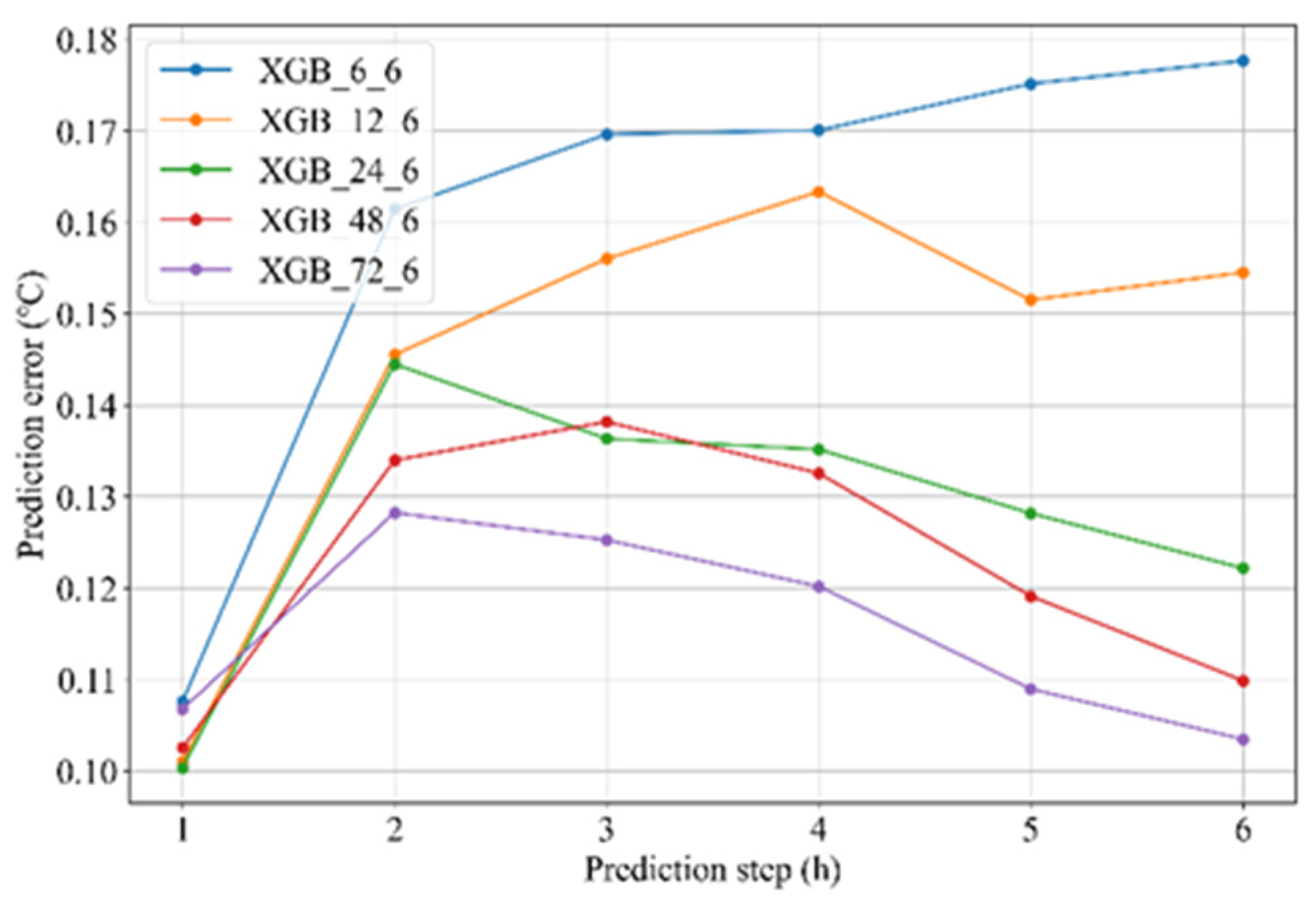
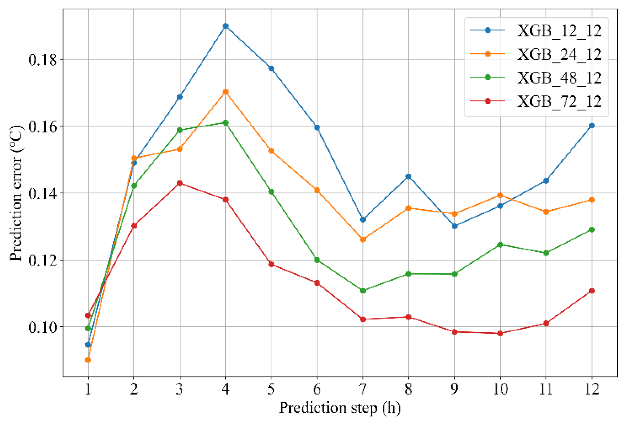
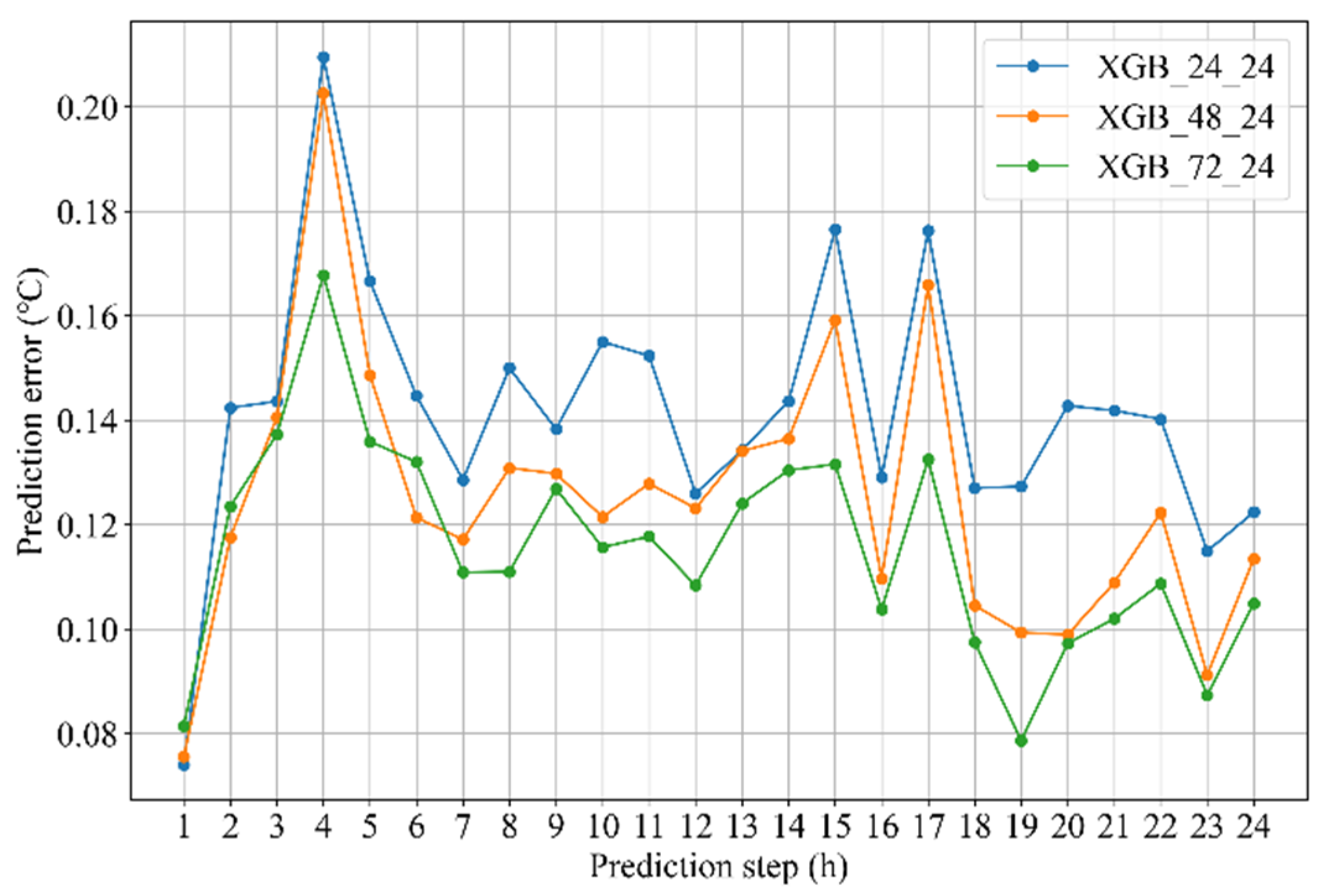
| 24 | 0.129 | 0.140 | 0.141 |
| 48 | 0.123 | 0.130 | 0.128 |
| 72 | 0.116 | 0.114 | 0.117 |
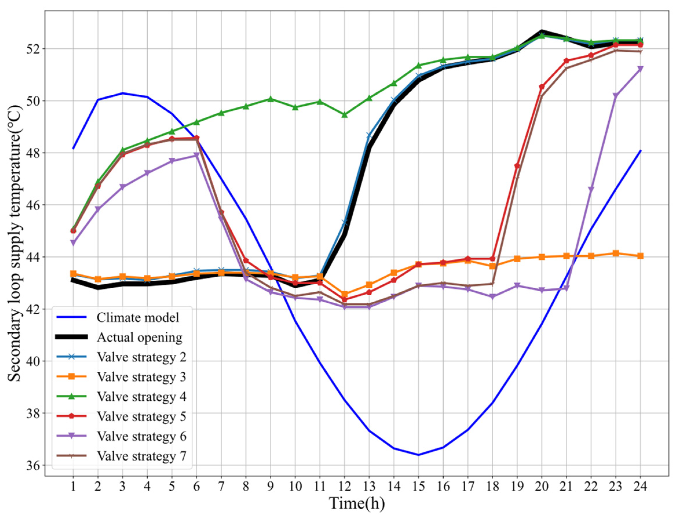
| Valve Regulation Strategy for the Next 24 h (%) | ||||||||||||
|---|---|---|---|---|---|---|---|---|---|---|---|---|
| 1 | 2 | 3 | 4 | 5 | 6 | 7 | 8 | 9 | 10 | 11 | 12 | |
| #1 | 15 | 15 | 14.8 | 15 | 15 | 15 | 15 | 15 | 15 | 15 | 15 | 18 |
| #2 | 15 | 15 | 15 | 15 | 15 | 15 | 15 | 15 | 15 | 15 | 15 | 15 |
| #3 | 20 | 20 | 20 | 20 | 20 | 20 | 20 | 20 | 20 | 20 | 20 | 20 |
| #4 | 20 | 20 | 20 | 20 | 20 | 20 | 15 | 15 | 15 | 15 | 15 | 15 |
| #5 | 18 | 18 | 18 | 18 | 18 | 18 | 10 | 10 | 10 | 10 | 10 | 10 |
| #6 | 20 | 20 | 20 | 20 | 20 | 20 | 8 | 8 | 8 | 2 | 2 | 2 |
| 13 | 14 | 15 | 16 | 17 | 18 | 19 | 20 | 21 | 22 | 23 | 24 | |
| #1 | 20 | 20 | 20 | 20 | 20 | 20 | 20 | 20 | 20 | 20 | 19.9 | 20 |
| #2 | 15 | 15 | 15 | 15 | 15 | 15 | 15 | 15 | 15 | 15 | 15 | 15 |
| #3 | 20 | 20 | 20 | 20 | 20 | 20 | 20 | 20 | 20 | 20 | 20 | 20 |
| #4 | 15 | 15 | 15 | 15 | 15 | 15 | 18 | 18 | 18 | 18 | 18 | 18 |
| #5 | 10 | 10 | 10 | 10 | 10 | 10 | 10 | 10 | 10 | 18 | 18 | 18 |
| #6 | 2 | 2 | 2 | 2 | 2 | 2 | 18 | 18 | 18 | 18 | 18 | 18 |
Disclaimer/Publisher’s Note: The statements, opinions and data contained in all publications are solely those of the individual author(s) and contributor(s) and not of MDPI and/or the editor(s). MDPI and/or the editor(s) disclaim responsibility for any injury to people or property resulting from any ideas, methods, instructions or products referred to in the content. |
© 2023 by the authors. Licensee MDPI, Basel, Switzerland. This article is an open access article distributed under the terms and conditions of the Creative Commons Attribution (CC BY) license (https://creativecommons.org/licenses/by/4.0/).
Share and Cite
Li, Z.; Luo, Z.; Zhang, N.; Lin, X.; Huang, W.; Feng, E.; Zhong, W. Investigation of Predictive Regulation Strategy of Secondary Loop in District Heating Systems. Sustainability 2023, 15, 3524. https://doi.org/10.3390/su15043524
Li Z, Luo Z, Zhang N, Lin X, Huang W, Feng E, Zhong W. Investigation of Predictive Regulation Strategy of Secondary Loop in District Heating Systems. Sustainability. 2023; 15(4):3524. https://doi.org/10.3390/su15043524
Chicago/Turabian StyleLi, Zhongbo, Zheng Luo, Ning Zhang, Xiaojie Lin, Wei Huang, Encheng Feng, and Wei Zhong. 2023. "Investigation of Predictive Regulation Strategy of Secondary Loop in District Heating Systems" Sustainability 15, no. 4: 3524. https://doi.org/10.3390/su15043524