1. Introduction
Past human activities or “footprints” are now commonly held responsible for the current pollution of the environment. The human footprint is measured by how fast humans consume resources and generate waste versus how fast Earth can absorb their waste and generate resources, according to [
1]. When it comes to an air emissions footprint, the greenhouse gases (GHG) emissions are the most widely analyzed as they allow the calculation of radiative forcing. When this radiative forcing is positive, the Earth system captures more energy than it radiates to space: it is a common measure for the global warming of the Earth [
2]. The calculation of this carbon footprint tends to account for all GHG emissions caused by an individual, event, organization, service, place, or product, and is expressed in units of carbon dioxide equivalent (CO
2-eq).
The annual meetings of the United Nations Climate Change Conference at the World Conferences of the Parties (COP) allow for a review of the objectives of the global effort to fight climate change. They assess GHG footprints at the global level and gather engagement of countries to limit CO2 emissions for fighting global warming and its impact on biodiversity. In line with these engagements, new definitions, laws, and methodologies for calculating and limiting these GHG emissions are voted at the country level, creating a new framework applicable to companies, the underlying hypothesis being that the country’s emissions are the sum of emissions coming from its inhabitants and its companies.
As such, listed and unlisted companies started reporting their emissions in their extra-financial communication. According to [
3], the carbon footprint of a company depends on the total amount of CO
2-eq that is directly and indirectly caused or accumulated over the life stages of its products. From the company’s point of view, the assessment of its GHG footprint can be useful not only for regulatory or accounting disclosure, but also for implementing strategies designed to mitigate and reduce its emissions. All frameworks like carbon pricing policies, measuring alignment to climate scenario with the Paris Agreement Capital Transition Assessment (PACTA), or moving toward net zero GHG emissions via Net Zero Banking Alliances (NZBA) need a correct GHG emissions baseline. This momentum will be emphasized by the new Corporate Sustainability Reporting Directive (CSRD) coming into force from 2024 for the largest companies to 2026 for Small and Medium-sized Enterprises (SME) in the European Union (EU). This directive will also apply to non-European companies, making over 150 million euros of turnover in Europe, according to the Council of the European Union. Companies will need to report audited GHG emissions as well as a quantitative pathway and remediation plan to cancel their net emissions.
Overall, these GHG emissions assessments measure exposure to transition risk and negative cash flows coming from fines or outflows to competitors with greener footprints. They are useful for fundamental financial analysis and slowly implemented in corporate valuation methodologies, at least for the most vulnerable sectors. Nevertheless, as soon as financial institutions aggregate GHG emissions at the portfolio level for several companies, they need homogeneous methodologies. At this stage, company reporting of GHG emissions is either voluntary or mandatory depending on location and is linked to defined nomenclatures (mostly activity types and size of companies). As explained previously, the calculation methodology is often defined along with the regulation and specified at the sector level. The heterogeneity of these methodologies can sometimes make comparisons among companies in different countries or sectors difficult and thus create biases. Moreover, not only may calculation methodologies vary, but they are also mainly not documented in the reports.
In the Global Warming Potential (GWP) framework, for any gas, CO
2-eq is calculated as the mass of CO
2, which would warm the earth as much as the mass of that gas: it provides a common scale for measuring the climate effects and global warming impacts of different gases. In practice, measuring the GHG emissions of a stakeholder requires much more information depending on how the GWP is released. To standardize these methodologies of calculation, the GHG Protocol, first published in 2001 [
4], is used by large companies, by the World Business Council for Sustainable Development (WBCSD), and the World Resources Institute (WRI). Even if, in some cases, companies report according to the ISO 14064 standards or the carbon-balance tool used in France, it has become the most widely used methodology in the world when it comes to assessing GHG emissions. The carbon inventory is divided into three scopes corresponding to direct and indirect emissions:
Scope 1: Sum of direct GHG emissions from sources that are owned or controlled by the company: stationary combustion, e.g., burning oil, gas, coal, and others in boilers or furnaces; mobile combustion, e.g., from fuel-burning cars, vans, or trucks owned or controlled by the firm; process emissions, e.g., from chemical production in owned or controlled process equipment, such as the emissions of CO2 during cement manufacturing; fugitive emissions from leaks of GHG gases, e.g., from refrigeration or air conditioning units.
Scope 2: Sum of indirect GHG emissions associated with the generation of purchased electricity, steam, heat, or cooling consumed by the company.
Scope 3: Sum of all other indirect emissions that occur in the value chain of the company, including financed emissions via investments.
Most current regulatory standards make reporting on scope 1 and scope 2 mandatory for large companies. Reporting on scope 3 is mostly optional or to be reported later in 2023 or 2024, even if scope 3, also referred to as value chain emissions, is often the largest component of companies’ total GHG emissions for some business industries like automakers or financial institutions. In practice, making the methods for calculating emissions in a given industry converge makes it easier not only to model but also to compare the emissions of each company with those of its peers.
To guarantee data quality of companies’ reported GHG emissions, independent bodies, such as the Carbon Disclosure Project (CDP), a not-for-profit charity that runs the global disclosure system or external auditors in extra financial Corporate Social Responsibility (CSR) reports, are more and more involved increasing convergence of methodologies and controls.
In this study, the methodology is limited to scope 1 and scope 2. Regarding scope 3 emissions, some framework like the Partnership for Carbon Accounting Financials (PCAF), officially recognized by the GHG protocol, allows measuring scope 1 and scope 2 emissions of a financial institution using reported emissions of investments sources but also estimates of scope 1 and 2, as stated in [
5].
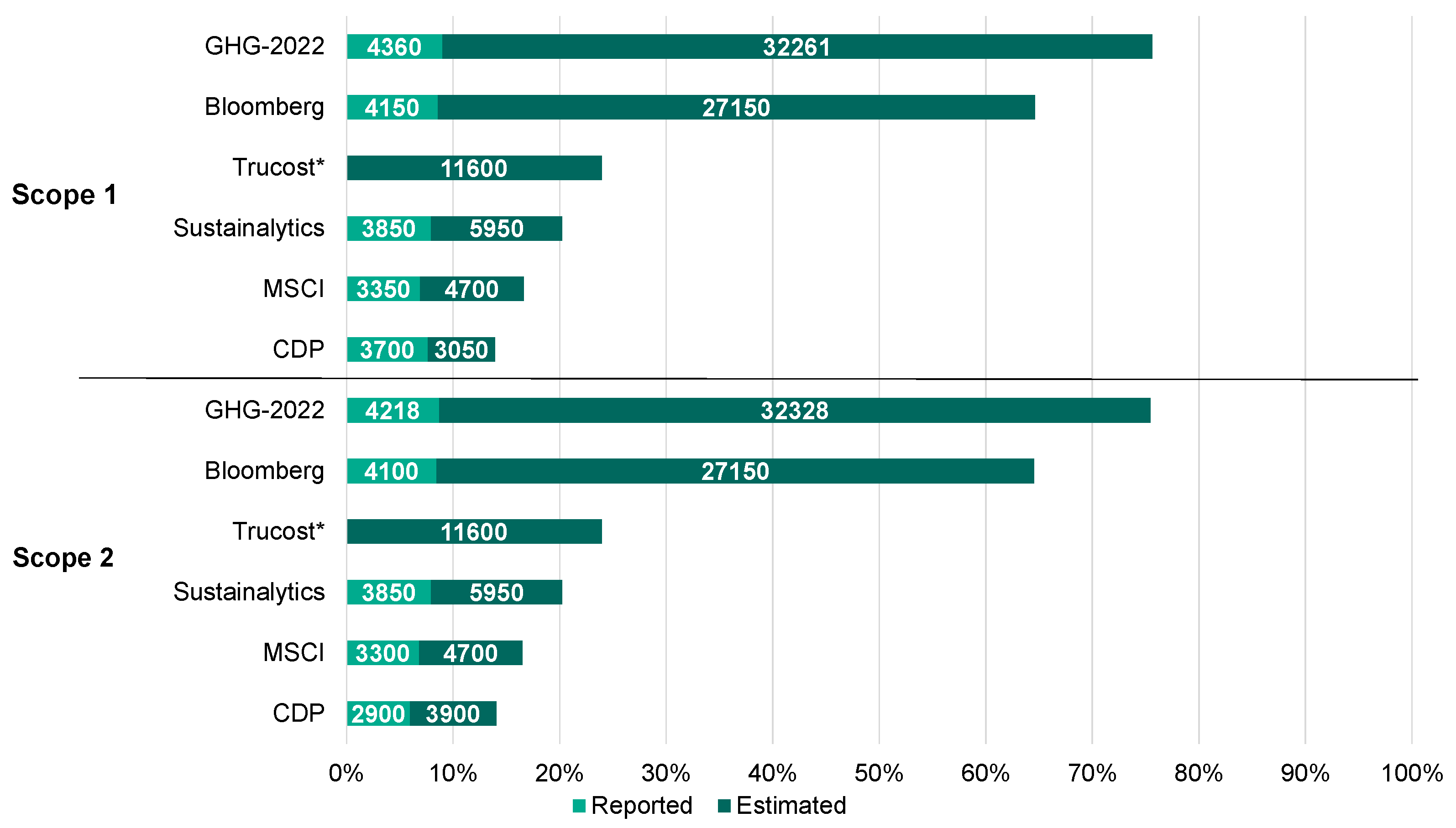
Overall GHG emissions from large firms in developed countries follow a common methodology for calculating scope 1 and 2 emissions: results are either published, validated, or both by independent bodies, such as external auditors, the CDP, or both. In 2021, this was the case for more than 4000 companies worldwide, as observed in this study. For a typical investment universe of 15,000 companies, this means that about 11,000 companies (73%) were not reporting their scope 1 and 2 GHG emissions. This breadth of reporting is not sustainable even in the short term, knowing the increasing number of regulatory bodies and investors who either want or are required to take into account the GHG emissions of companies. At the same time, even some recent studies like [
6] analyze GHG emissions of 14,468 companies, including 98% of publicly listed companies, without mentioning or analyzing that 80% of the data used is coming from GHG modeled estimates from the data provider Trucost. They even construct a regression model to fit all the scopes 1, 2, and 3 data and draw conclusions on global carbon premiums in the market. On the opposite, some studies using the same Trucost dataset specify and analyze more deeply the underlying quality of the GHG emissions data used, like [
7].
That is why it is so important to analyze in detail the corporate GHG emissions data: operational scopes (accounting consolidation scope, some of biggest factories), standards of calculations (GHG protocol or others), calculation basis (scope 2 Market-based versus Location-based) and this, even if the data is modeled (simple derivation from a previous year to more complex non-linear models). When it comes to comparing corporations across geographies and sectors or drawing conclusions at the global level for anthropogenic GHG emissions, we need a fair assessment of the GHG emissions at country, corporation, factory, and personal levels.
This study focuses narrowly on the unreported estimated emissions of companies. The model framework focuses on estimating the targeted high-quality GHG emissions, especially waiting for international regulatory bodies to bring a homogeneous framework for corporations to report their GHG emissions in extra financial statements. For financial use cases needing GHG emissions for portfolio construction, there is also a distinction to be made between point-in-time estimates using only information available at the date of the estimated emission and “as-of-today” estimates using all available information, including those posterior to the date of the estimated emissions. These two types of estimates answer different use cases and require different calibration strategies.
2. Literature Review—Hypothesis
Focusing on scopes 1 and 2, the available reported data is typically issued from voluntary reporting based on the CDP or on extra financial reports (CSR reports) from companies. With a few exceptions, like France with Article 173 of the French Energy Transition law, GHG emissions reporting is not yet mandatory, but the corporate regulatory framework to report GHG emissions was improved recently with the CSRD in the EU or the Securities and Exchange Commission (SEC) proposed rules in the United States [
8].
Corporate GHG emissions models make the link between the industrial processes of each business model and the carbon emissions associated with each stage of those processes. The Environmental Input Output Analysis (EIO) and the Process Analysis (PA) models give precise results for a given industrial process [
9]. However, neither the information required to quantify companies’ use of those processes nor their intensity in the overall annual production chain, is publicly available. Linking detailed industrial processes and technologies with an accounting of GHG emissions is a perilous task, even when it is handled by big corporate sustainability expert teams or by CDP experts.
To mitigate such a lack of data, financial data vendors rely on relatively simple models to estimate GHG emissions for some companies that do not currently report. These estimates are usually sector-level extrapolations based on indicators, such as the number of employees and income generated, or both. Sector averages or regression models constructed from the existing reported GHG emissions data from peer companies have the advantage of simplicity for explainability, but the number of regressors is usually limited, as are the sample sizes. Model validation tends to rely on the quality of the regression in-samples where data is available.
Data providers, such as Bloomberg [
10], MSCI ESG [
11,
12,
13], Refinitiv ESG—previously known as Thomson Reuters ESG–[
14,
15,
16] and S&P Global Trucost and CDP, use models to estimate the GHG emissions of companies that fail to publish emissions data. Such models rely mainly on rules of proportionality between emissions and the size of the company operations or, more recently, on more complex approaches using non-linear models. The simple models tend to use historical data available for the industry as a basis for the calculation, and focus on predicting the logarithm of GHG emissions. Occasionally, they also use energy-specific metrics like GHG intensity per the company’s energy consumption and production or per ton of produced cement. However, these metrics are only available for the limited number of companies reporting them without reporting their GHG emissions. These models are calibrated on samples of reported data. Performance is around 60% in terms of
for most samples when evaluating the logarithm of the emissions. To be noted, these performance levels are tested in-the-sample, meaning the
computed with the logarithm of the GHG emissions is tested with the data used to calibrate the model. The performance of the model is calculated on the same companies used for the calculation of the regressions levels. On the other hand, out-of-sample performance tests require a completely new dataset to test the model on unseen companies with reported emissions. Good out-of-sample performance shows that the model avoids overfitting and is able to generalize well.
Some more advanced models described in [
17,
18,
19] proposed the use of Ordinary Least Squares (OLS) and Gamma Generalized Linear Regression (GGLR) with a broader dataset of publicly available company data for the construction of models. Such models go beyond using just simple factors and rely more on data correction processes or smaller sub-samples of industries where the models work correctly. These models are more effective than the previous ones, with in-the-sample
computed with the logarithm of the GHG emissions around 80%.
More recently, two studies proposed the use of statistical learning techniques to develop models for predicting corporate GHG emissions from publicly available data. These machine-learning approaches take the form of:
In [
20], a meta-learner relying on the optimal set of predictors combining OLS, Ridge regression, Lasso regression, ElasticNet, multilayer perceptron, K-nearest neighbors, random forest, and extreme gradient boosting as base learners. Their approach generates more accurate predictions than previous models even in out-of-sample situations, i.e., when used to predict reported emissions that were not used to construct the model. Nevertheless, the strongest predictive efficiency of the model was found for predicting aggregated direct and indirect emission scopes as opposed to predicting each of them separately. Furthermore, despite the improvement over existing approaches, the authors also noted that relatively high prediction errors were still found, even in their best model. Indeed, the five dirtiest industries representing about 90% of total scope 1 emissions (Utilities, Materials, Energy, Transportation, Capital Goods) have an average in-the-sample
computed with the logarithm of the GHG emissions of only 51%. The five dirtiest industries accounting for about 70% of the total emissions in terms of scope 2 (Materials, Energy, Utilities, Capital Goods, Automobiles & Components) have an average in-the-sample
computed with the logarithm of the GHG emissions of only 52%. In addition, their model fails for Insurance, both for scope 1 and scope 2, with
of −378% and −151%, respectively. Moreover, extrapolating these results to a typical wider investment universe is difficult since their used GHG emissions dataset is small, with around 2300 reporting firms against 4300 in this study. The paper also lacks discussions on the achievable coverage of GHG emissions estimates and on the interpretability of the model, with no explanation of why it outputs such estimates.
In [
10], amortized inference with Gradient Boosted Decision Trees (GBDT) models [
21], re-calibrated using Conditional Mixture of Gammas and Mean Maximum Discrepancy (MMD)-based patterned dropout for regularization. The model is trained on hundreds of features, including Environment, Social, and Governance (ESG) data, fundamental data, and industry segmentation data. The GBDT allows for non-linear patterns to be found even if not all data features are available. Moreover, an important debiasing approach compares the feature distributions for the reporting companies and non-reporting companies by trying to match missing features between labeled data and unlabeled data using MMD. In this model, the
computed directly with the GHG emissions goes from 84% for firms with good disclosures (lots of features available) to 41% for companies with average or poor features disclosures. That paper especially lacks transparency, with several implementation elements like the choice of features not explained, making it not reproducible. That paper also lacks a discussion on the interpretability of the designed model.
Understanding the risks and opportunities arising from the GHG emissions of companies requires good financial and non-financial data. In some countries and for some companies, as long as GHG emission reporting and auditing is not compulsory, the only viable alternative is to predict non-reported company emissions relying on estimation models. From the above, the current state-of-the-art does not yet provide good enough models for the task at hand. In our view, the quality of data made available by the specialized data vendors is not yet sufficient. Understanding the reasons behind this problem and being able to propose alternative approaches that can lead to better models and more accurate predictions of unreported data is thus of great importance.
The recently proposed approaches by [
10,
20] based on statistical learning, offer a promising starting point. The central challenge with such statistical learning approaches is to strike the right balance between increasing both the model complexity and accuracy while limiting the risk of overfitting. In this paper, we propose a statistical learning model to predict unreported scope 1 and scope 2 company emissions in an investment universe of about 50,000 companies, of which only about 4000 companies actually report. This model is inspired by the work of [
22] and aims at achieving the following qualities:
accuracy, globally and by granular sub-sectors, with good and balanced performances on each sub-sector’s on point-in-time estimates.
operability, transparency of the methodology, and reproducibility of results, keeping the complexity of the model to a minimum while achieving good global and granular performances. For example, all data preprocessing steps must be fully automated with no manual corrections. The model of this study is flexible and easily allows the inclusion of new input data with the evolution of regulations, especially on GHG disclosure.
large final coverage, aiming at using the model for a scope of 50,000 companies, both public and private, including small ones.
interpretability, a regulatory requirement as highlighted by [
22]. The model of this study provides clear and exhaustive statistical explanations of the outputs.
To succeed, we made some significant choices in departing from existing approaches. First, models are always tested on data samples never seen during the calibration, so that their generalization abilities can truly be measured, which was not done in [
22]. The second important decision was to always evaluate the model globally and by the granular sub-sector, country, and bucket of revenues. Obtained estimates are also compared to the ones from other providers through a detailed methodology. To our knowledge, this paper is the first to propose evaluating the model at such levels of granularity. The third important decision was to keep the raw dataset from data providers with a totally documented and fully automated data preprocessing and no manual corrections. Even if the use of incorrect data can reduce the accuracy of models, it allows for full reproducibility and industrialization, as this latter brings some operational constraints to produce automated updates of the model. We also introduce shortly an automated data polishing process at the end of this study. The fourth important decision was to keep model complexity to a minimum by relying only on a fixed small set of predictive features and the most accurate non-linear machine learning approaches without losing interpretability. As a matter of fact, the last important decision was to make a fully interpretable model using a model-agnostic method so that interpretability does not come at the expense of performance. Indeed, for instance, the implementation from [
22] required keeping a linear layer in the model, degrading accuracy. To our knowledge, such an extensive part on the interpretability of a machine learning model estimating GHG emissions has not been done in the current literature and allows us to understand why the model produced such emissions values.
In the remainder of the paper, we describe the data retained to calibrate and evaluate our model and present the designed methodology in-depth, insisting on the particular implementation choices made, necessary to apply it to the use case of estimating GHG scope 1 and 2 emissions. We then discuss the results associated with this methodology both by comparing our estimates to true GHG emissions reported by companies and by comparing our estimates to the ones from other providers. Finally, we provide tools to understand how the constructed model works and why it estimates such values of GHG emissions.
4. Methods
4.1. Problem Settings
The goal of this study is to develop a data-driven model estimating scope 1 and scope 2 greenhouse gas emissions of companies that have never reported them. Using the vast amount of available indicators, whose selected ones have been exhibited in
Section 3, we build a high-quality dataset and calibrate a machine learning model that outputs the estimated emission of a company. This automated method allows the estimation of the emissions of any company as long as enough financial and non-financial data is available. Scope 1 and scope 2 emissions are estimated through two separate models.
This is a regression setting: the model learns for each possible couple the reported emission from a set of P potentially explanatory factors called features. Here, i represents a company, and t is the year of sampling of the features and emissions. Let us relabel all the couples by the index . This regression problem consists in estimating , the reported emission, with a vector with P components, or equivalently, to explain the vector from the lines of matrix . Y is called the target and X the features matrix.
Optimizing a machine learning model supposes the division of the full dataset into three parts called the training, validation, and test sets:
The training set is used to optimize the parameters of the machine learning model on a set of features associated with their GHG emission. Practically, it learns the mapping between the lines of X and the components of the vector Y.
The validation set allows optimizing the model hyperparameters.
The test set is used to evaluate the generalization capacities of the model on data samples never seen in training or validation. In inference, the model takes as input a vector of features and outputs the estimated GHG emission.
The state of the art for regression problems on tabular data like this one is provided by Gradient Boosting models [
21], as shown for instance in [
23]. Gradient boosting consists in using a sequence of weak learners, making wrong predictions, that iteratively correct the mistakes of the previous ones, eventually yielding a strong learner, making good predictions. We use here decision trees as weak learners: we are using the GBDT algorithm. Different implementations of the GBDT method have been proposed, e.g., XGBoost [
24], LightGBM [
25], and CatBoost [
26]. We use LightGBM. The advantage of such methods with respect to linear regression is that they are able to learn more generic functional forms.
The model is trained to minimize the mean-squared error (cost function), also referred to in this paper as MSE, defined as
where
is the predicted output from the model (decimal logarithm of the GHG estimation, as explained in
Section 4.2.2) and
is the ground truth (decimal logarithm of the reported emission).
4.2. Target Computation
4.2.1. Raw Target Obtention
The explained variable, the reported GHG emissions for scopes 1 and 2, are sourced using two databases:
When both data sources are available for a company and year, CDP data is prioritized over Bloomberg. Indeed, Bloomberg GHG data is directly sourced from companies’ extra-financial communications. Norms and audit processes for these data may differ per country, whereas CDP used a uniform and audited process, based on the GHG Protocol [
4], for all companies in the world. Their reported emissions are expressed in tCO
2-eq.
4.2.2. Target Cleaning Procedure
GHG emissions are reported on different dates during the year. To unify samples and preserve meaning with the used training features, GHG emissions reported between January and June of the year y are attributed to the year , and the GHG emissions reported between July and December of the year y are attributed to the same year y. For both scopes, only one reported GHG emission per company and per year remains.
Variability is an important characteristic of GHG emissions data, leading sometimes to inconsistencies, with important changes in emissions for a company over the years: this could be due to changes in the reporting methodology, to a corporate action like the acquisition of a subsidiary or mergers. The chosen cleaning procedures mitigated these issues: a fully automated jump-cleaning methodology was developed.
We call jump a year-to-year variation in the GHG emission reported value of a company bigger than a threshold of 50%. This jump processing procedure aims at spotting jumps inside the dataset, removing all inconsistent points unless they can be explained by a significant corporate action. We make the hypothesis that the most recent data is the highest quality one: if an unexplained jump is detected in the time series of GHG emissions of a company, all data points before the jump and the jump are removed. A jump is unexplained if a concomitant and large enough corporate action to justify it cannot be found. In practice, a jump is said to be explained if, using a Bloomberg corporate action dataset, there exists at least one corporate action amounting to at least 20% of the company revenues during the year before or after the considered jump. The different thresholds were determined using trial and error.
To reduce the negative impact of the skewed nature of the GHG emissions distribution, the model is trained to estimate the decimal logarithm of the GHG emissions instead of the raw value. Another advantage of using the decimal logarithm resides in the interpretation of the estimated value: an error of one unit in the decimal logarithm estimation means an error of one order of magnitude (power of 10) in the raw GHG. For some use cases in the financial world and depending on the practitioner, having estimated the right order of magnitude for the GHG emissions can be enough. This study goes further in terms of performances but keeps this interpretability idea.
4.3. Training Features
For each of the obtained targets, a vector of features using the data sources exposed in
Table 1 is fetched. We trained a different model for each scope: two feature matrices are obtained, representing the training features for each of the scopes. The scope 1 training set has 16,234 samples, and scope 2 has 16,925. In
Table 2 and
Table 3, we summarize the 21 features used to train the model as well as their distribution and average coverage in the two training sets. In the remainder of this section, we provide details on these different features. Missing values are left as such: in addition to the capacities of the LightGBM implementation to handle them, it is the setting for which the best performances were obtained as opposed to the data imputation used in [
20,
22].
4.3.1. Financial Features
The model relies on financial features, allowing a better understanding of the size of a company and its assets. The Capital Expenditure, Enterprise Value, Gross Property Plant & Equipment (GPPE), Net Property Plant & Equipment (NPPE), and Revenue features are obtained annually for each company for which there is a target, meaning a reported GHG emission for scope 1 and/or scope 2. Both GPPE and NPPE are included as they both give elements on the tangible assets of a company that is physically responsible for its emissions (scope 1 and 2): the difference between the two is accounting elements linked to the age of the assets, that provide interesting information to the model. These values are converted from the reporting currency to dollars using the foreign exchange rate from the 31st of December of the considered year. Apart from this conversion, financial data are used as reported from the company’s financial communication with no additional manual re-treatment, guaranteeing reproducibility.
The last financial feature, the Life Expectancy of Assets, is obtained following [
18,
20], using the following formula:
The idea behind this proxy is to estimate the average life expectancy of the assets of a company by dividing the total amount of tangible assets of a company by the depreciation expense the company reported for the considered year. We make the hypothesis that a company whose assets have a longer life expectancy are, on average, older and may emit more GHG.
As the Depreciation Expense indicator is not available and the Gross Property Plant & Equipment feature have many missing values, the equivalent following formula is used:
The numerator is modified by decomposing the Gross Property Plant & Equipment term. If the Capital Expenditure or Accumulated Depreciation indicators are missing values, they are ignored, and their values are set to 0. The denominator is modified by adding the depletion and amortization expense. We did not measure any significant impact of these approximations on the final GHG emission estimation.
4.3.2. Industry Classification
Industry classification and sectorization features allow the model to grasp the business model of a company; it is one of the most judgmental features used in GHG estimation models, truly distinguishing between companies by the nature of their activities according to their sectors. Indeed, the GHG emission profiles of companies operating in different sectors are not the same. For instance, sustainable energy companies are specifically tagged as such in some classifications and are not in others. There exist numerous industry classifications, grouping companies differently, which is critical for the model as it must not rely on a classification that would, for instance, never make the difference between companies operating in the Oil & Gas, Renewable Energy, or Nuclear fields. As a preliminary work, four typical business classifications were identified: The Refinitiv Business Classification (TRBC), the Standard Industrial Classification (SIC), the Global Industry Classification Standard (GICS), and the Bloomberg Industry Classification Standard (BICS). Testing these different classifications and different combinations of them, we retain the one for which the model gave the best performances in terms of MSE by subsectors, the BICS. No manual retreatment is done for reproducibility purposes.
For each company, its main industry classification is obtained using the BICS. The industry in which a company is classified corresponds to the one in which it is making the biggest fraction of its revenues. The BICS classification is a detailed and granular one, with seven hierarchical levels. It makes granular distinctions between the different sectors, going as far as distinguishing companies operating in the Oil & Gas Production field but either working on Petroleum Marketing or focusing on Exploration & Production.
With the important level of details of the BICS classification, the deeper levels are not dense enough in the training dataset: not all companies have data for levels 5, 6, or 7 in the classification. As a result, having just a few instances of a particular industry at a deep level is only adding noise to the model and making it more prone to overfitting, the model has more difficulties to generalize to other samples. In the preprocessing steps, all occurrences of industries that are present less than 10 times in the training set are removed. They are replaced with a NaN value, missing values being directly handled using the LightGBM model.
As precise as the BICS classification is, it is complemented by the New Energy Exposure Rating from Bloomberg. It is a categorical feature that estimates the percentage of an organization’s value that is attributable to its activities in renewable energy, energy smart technologies, Carbon Capture and Storage (CCS), and carbon markets. This categorical data can take five values:
A1 Main driver: 50 to 100% of the organization’s value is estimated to derive from these activities.
A2 Considerable: 25 to 49% of the organization’s value is estimated to derive from these activities.
A3 Moderate: 10 to 24% of the organization’s value is estimated to derive from these activities.
A4 Minor: less than 10% of the organization’s value is estimated to derive from these activities.
NaN if missing.
4.3.3. Energy Data
Energy features, expressed in GWh, are often directly correlated to GHG emissions and allow the model to have a better understanding of how a company is using its assets. Energy Consumption is the amount of energy consumed by a company during a year. Total Power Generated is the energy produced in a year by a company, and therefore, it is only relevant for companies in some specific industries, explaining the low coverage shown in
Table 3. To be noted, the distinction between renewable and non-renewable power generated is available in our dataset but was not used in this version of the model. The reporting period may differ between companies: similarly to the GHG emission targets, values reported between January and June of the year
y are attributed to year
, and those reported between July and December of year
y are attributed to the same year,
y.
4.3.4. Regional Data
Regional data allows the model to get a sense of the environment the company is operating in, for the country in which it is incorporated. The Carbon Intensity of Energy Mix refers to the CO2 Emissions from fuel combustion for the country in which the considered company is incorporated. Data is gathered from the International Energy Agency (IEA). Depending on when these data are obtained, there may be missing data for the most recent years; in this case, the time series for the considered country is extended using the last known value.
The model also relies on a categorical feature describing whether a system of carbon taxes or an Emission Trading System (ETS) has been put in place at a national or sub-national level. This feature, called CO2 Law, can take three values:
No CO2 law: no carbon tax or ETS has been put in place for the considered country;
National Implemented: one or both of these systems are implemented in the whole considered country.
Sub-national Implemented: one or both of these systems are implemented in part of the considered country (a state in Canada or in the USA for instance).
4.4. High Quality Dataset
Using the features and target cleaning procedures, the final training datasets to estimate scope 1 and scope 2 GHG emissions are obtained. All preprocessing steps are transparent and fully automated with no manual retreatment for the sake of reproducibility. These two high-quality datasets are used in all the remaining parts of this study.
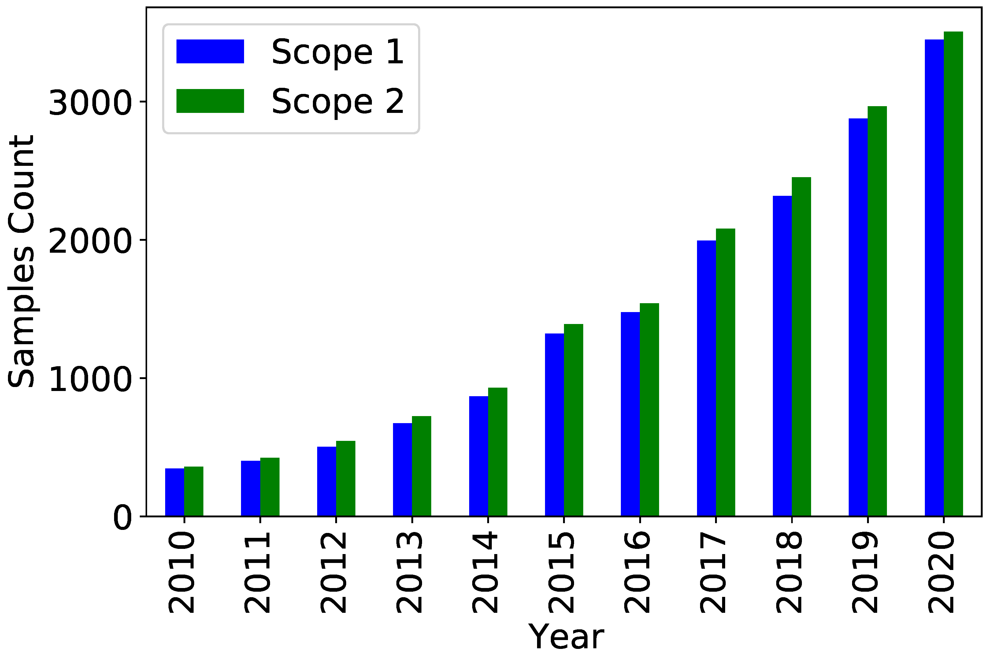
Figure 1 shows for scope 1 and scope 2 the number of companies for which a reported GHG emission per year was obtained. There has been an important increase in data quantity through the years, which illustrates the growing importance of GHG emission reporting.
4.5. Cross-Validation and Hyperparameter Tuning—Out-of-Sample Performance Evaluation
The usual strategy in machine learning for time series consists of a single data split into a causal consecutive train, validation, and test data sets. The model learns the mapping between features and targets on the training set, determines its parameters on the validation one, and is finally tested in test one. To avoid overfitting and preserve the generalization capacity of the model, the test set should only be used at the end of the training, to evaluate the model. This usual strategy is not appropriate for the current problem, estimating the GHG emissions of companies that have never reported them. Indeed:
the usual splitting scheme does not comply with the use case: the goal is not to predict future GHG emissions but to estimate unreported ones during the last available year.
the amount of data grows from a very low baseline both quantity- and quality-wise. The oldest data are not exploitable alone: using this splitting scheme would lead to unreliable results as only old data would be in the training set. To get meaningful results, we need to rely on the entire time span of available data.
similarly, GHG emissions data are non-stationary, leading to inaccurate results using this standard splitting scheme.
To address these issues, a specific testing methodology and cross-validation scheme were developed, inspired by [
27].
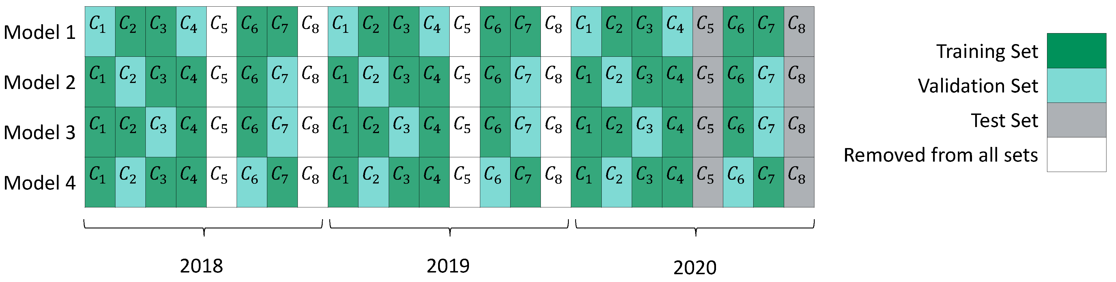
To estimate unreported data during the last available year, the test set built to evaluate the models should only include companies that are not in the training or validation sets: the goal of the model is to estimate unreported emissions of companies which, most of the time, never reported their emissions before. Moreover, it avoids a potential bias: because of the huge year-over-year correlation of GHG emissions for the same company, having the same company both in training/validation and in tests during different years would lead to an overfitted model. In practice, the test set is built by selecting 30% of the companies for which there is a reported value during the last available year: these samples constitute the test set. These companies may have other reported emissions for other years: all these companies are removed from the training and validation sets.
For training and validation, a K-fold company-wise cross-validation is used: 80% of companies are randomly assigned to the training set and the remaining 20% to the validation one. We train 180 models on each of the K training sets varying the hyperparameters of the LightGBM algorithm and select the best one based on its average performances, measured using the MSE, on the respective validation sets. In this way, the current framework is respected, not having any company both in training and in validation, and models are trained with a large part of the most recent and more relevant data, while also validating them with the most recent and more relevant data. We take .
Figure 2 illustrates in a three-year and eight-company dataset the procedure used to build the training, validation, and test sets.
7. Interpretability of the Model: Understanding Why It Outputs These GHG Emissions Estimates
The interpretability of machine learning models producing GHG emissions is becoming a regulatory element. In this part, we provide tools to interpret how the model works and why it estimates such values of GHG emissions; a breakdown of the impact of the different training features on the estimated emissions is computed.
A common critic of GBDT is that, despite their superior performances in tabular settings, they remain difficult to interpret. A tool, recently applied to the machine learning field and called Shapley Values, solves this issue. Shapley values, first introduced in the context of game theory [
28], provide a way in machine learning to characterize how each feature contributes to the formation of the final predictions. Shapley values and their uses in the context of machine learning are well-described in [
29].
The Shapley value of a feature can be obtained by averaging the difference of prediction between each combination of features containing and not containing the said feature. For each sample in the dataset, each feature possesses its own Shapley value representing the contribution of this feature to the prediction for this particular sample. Shapley values have interesting properties, like the efficiency property. If we note
the Shapley value of feature
j for a sample
and
the prediction for the sample
, Shapley values must add up to the difference between the prediction for the sample
and the average of all predictions
and then follow the following formula:
The dummy property states that the Shapley value of a feature that does not change the prediction, whatever combinations of features it is added to, should be 0.
Shapley value calculation is quite time- and memory-intensive. [
30] and later [
31] proposed an implementation of a fast algorithm called TreeSHAP, which allows approximating Shapley values for tree models like the LightGBM and which is used in the following. Shapley values computed with this algorithm are referred to as SHAP values.
7.1. SHAP Feature Importance
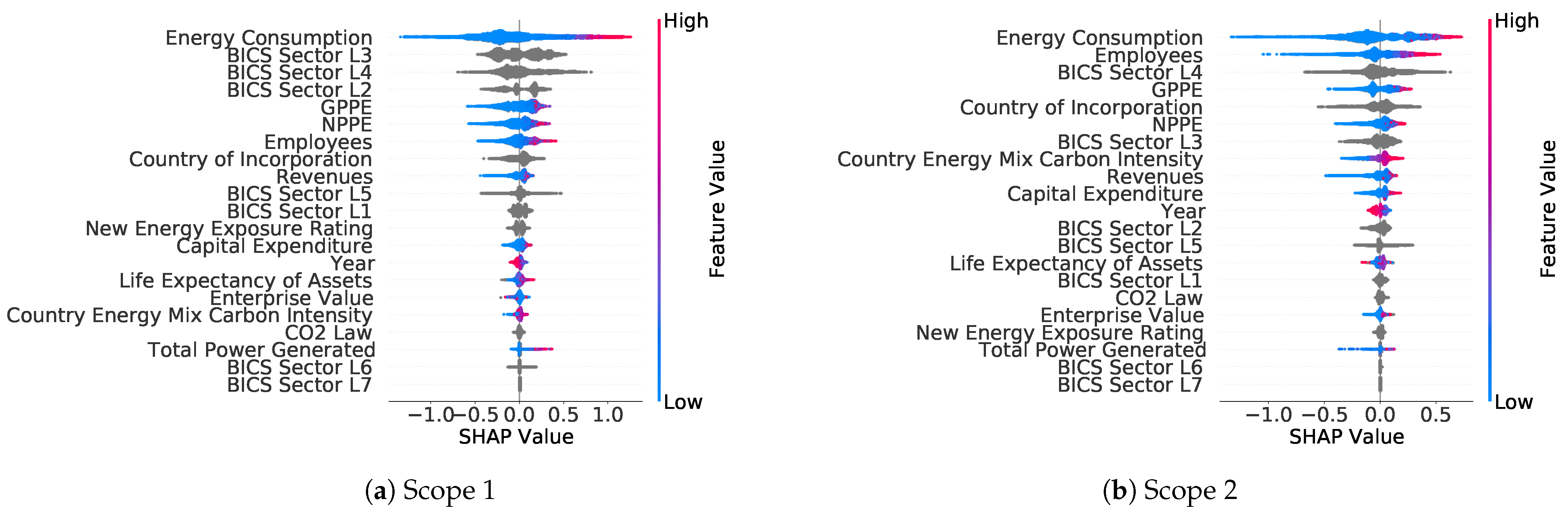
We provide in
Figure 7 the breakdown of SHAP values per feature for the scope 1 and scope 2 GHG emissions, ordered by importance. For each feature, this graph shows the distribution of SHAP values across each sample in the training set. These graphs are key elements in the constructed model as they make it interpretable: they can be computed for any set of features, allowing us to understand why the model makes a specific decision and outputs this predicted estimate.
The Energy Consumption feature is the most important one used by the model for both scope 1 and scope 2. As expected from the definition of scope 2, the Employees, Country of Incorporation, and Country Energy Mix Carbon Intensity features are more important for the estimation of scope 2 than the estimation of scope 1. The plot also highlights that the Business Classification features are paramount in GHG estimation models, with high importance for several levels of the BICS classification both for scopes 1 and 2; it was important to choose a granular classification as features up to the classification Level 6 were used. However, the too deep Level 7 of the BICS was not used by the model: as this Level 7 was too sparse, it did not bring additional information. The plots also show that the addition of the New Energy Exposure Rating complements well the BICS classification and contributes to the formation of the estimates.
Knowing these SHAP values not only allows us to better understand the estimates of the model output but also to evaluate the reliability of the estimates based on the presence or the absence of a feature: if the Energy Consumption feature is not given for a sample, it would lead, for certain sectors, to a less reliable estimate. This can be evaluated further by comparing the distribution of SHAP values for a set of companies that reported this feature and another set of companies which did not.
7.2. Relationship between Features Values and GHG Estimates
7.2.1. Numerical Features
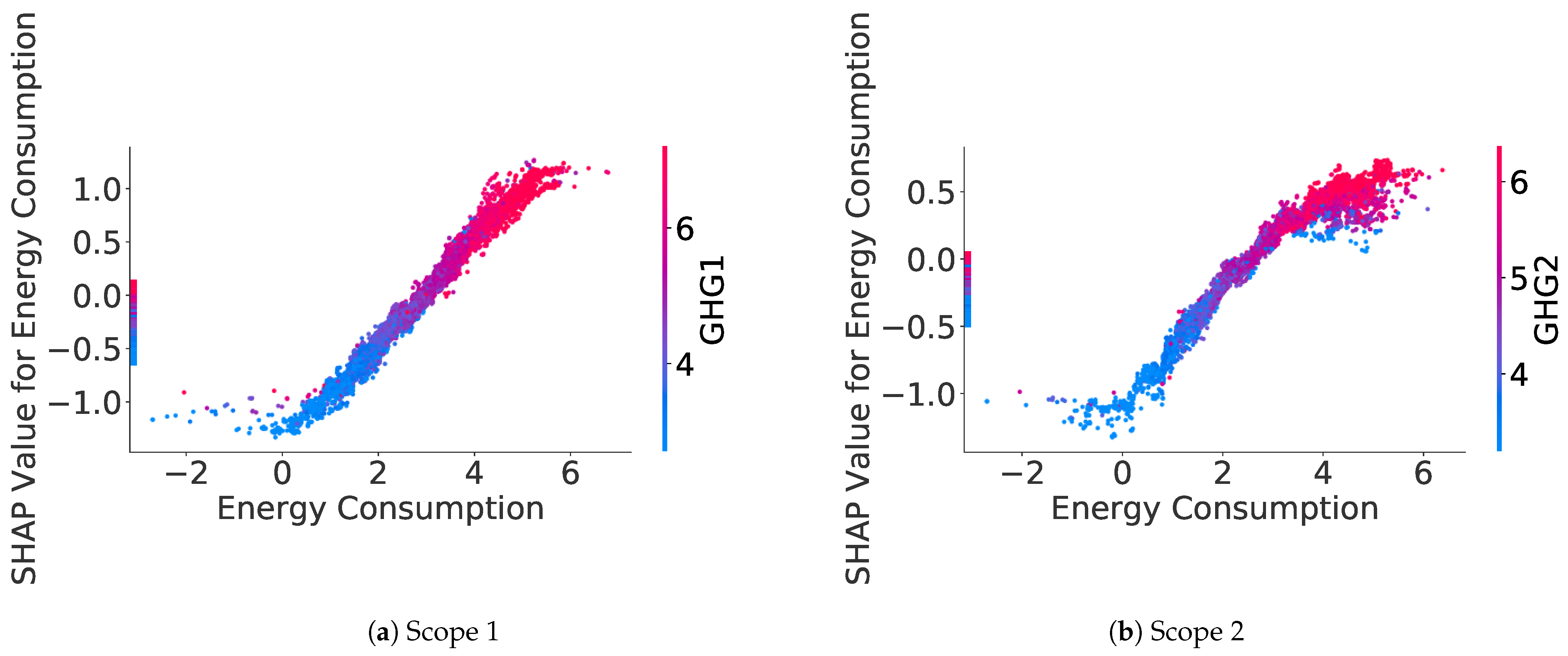
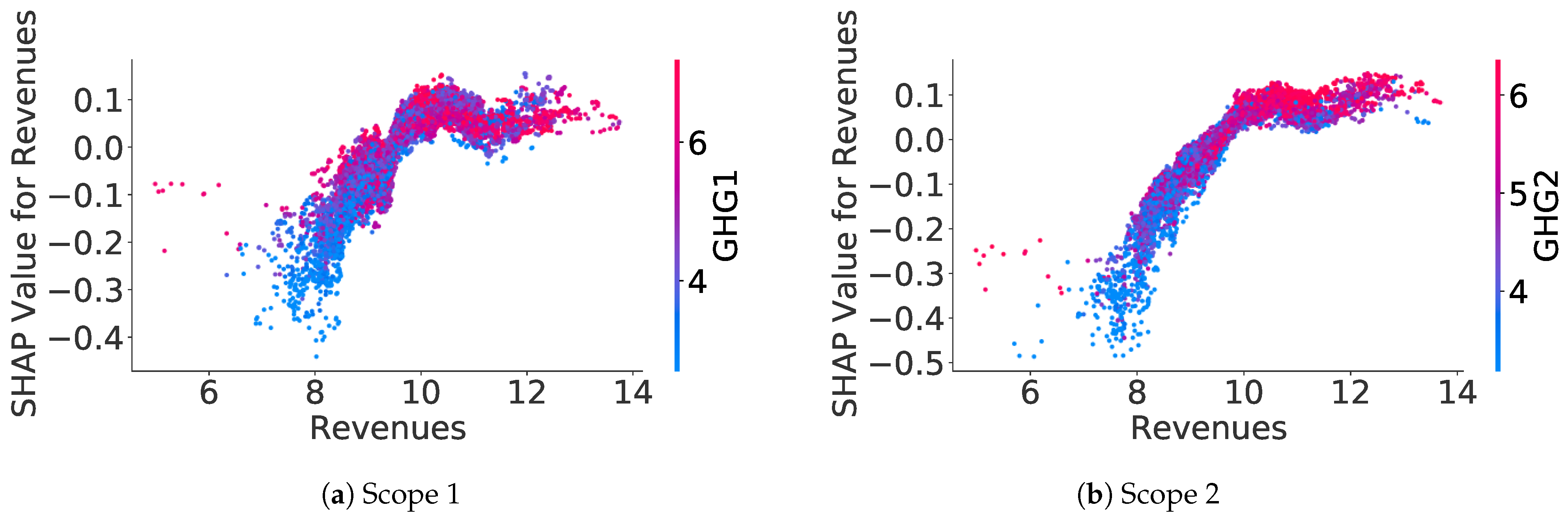
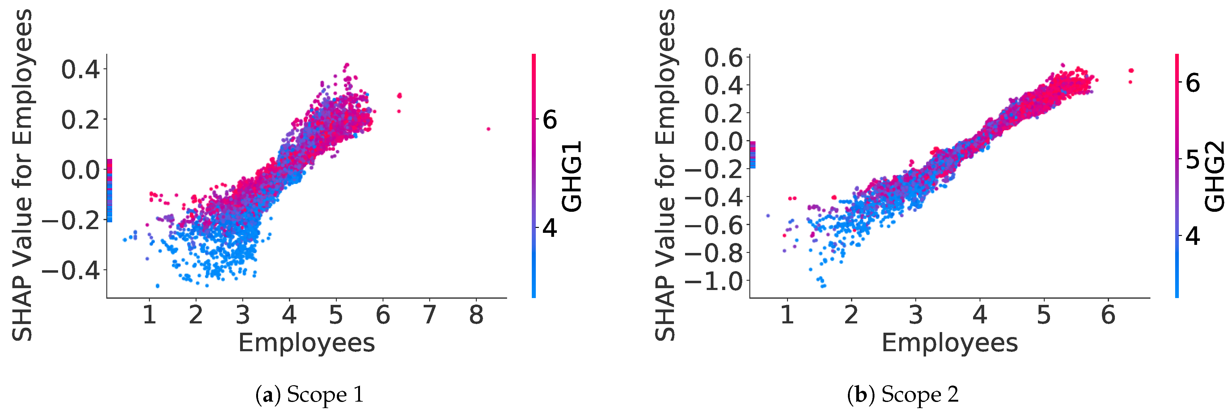
SHAP values can be computed for each feature on each sample, allowing us to understand the relationship captured by the model between a feature and the estimated GHG emission. Indeed, for numerical features, we can plot the SHAP values for a specific feature against this feature value in the dataset. For instance,
Figure 8 shows the relation between SHAP values of the Energy Consumption feature and the decimal logarithm of the Energy Consumption feature value. Apart from the points, which are on the Y-axis and which represent missing values for the Energy Consumption feature, there is, for both scopes, a near-linear increasing relationship between the SHAP values of the Energy Consumption feature and the decimal logarithm of this feature value.
Appendix B.1 provides some other examples of SHAP values plots for numerical features, allowing for a better interpretation of what the model is learning.
7.2.2. Categorical Features
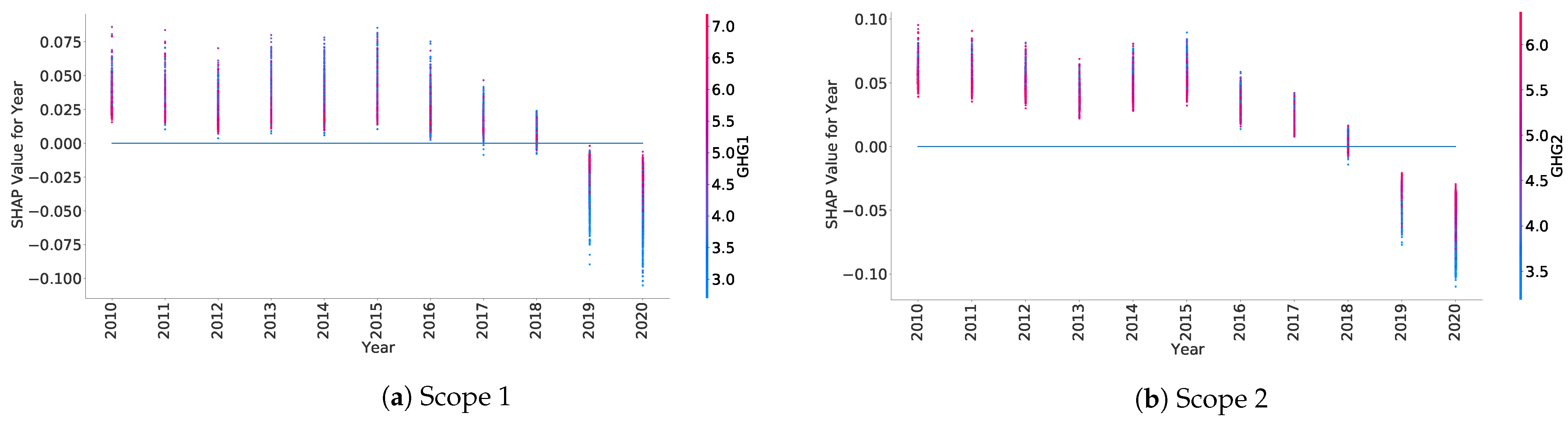
SHAP values can also be used on categorical features to study their distribution, for each value a categorical feature can take. For instance,
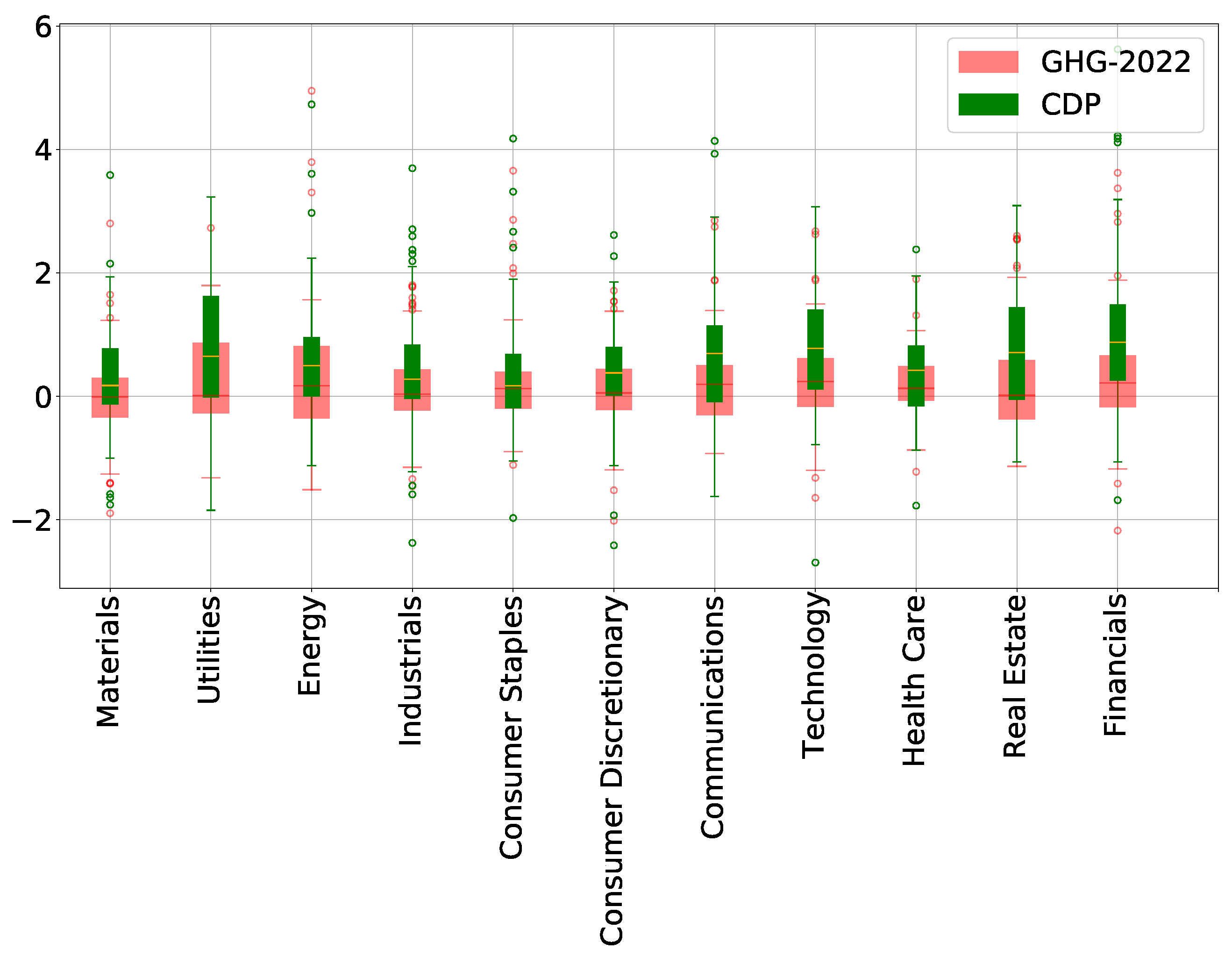
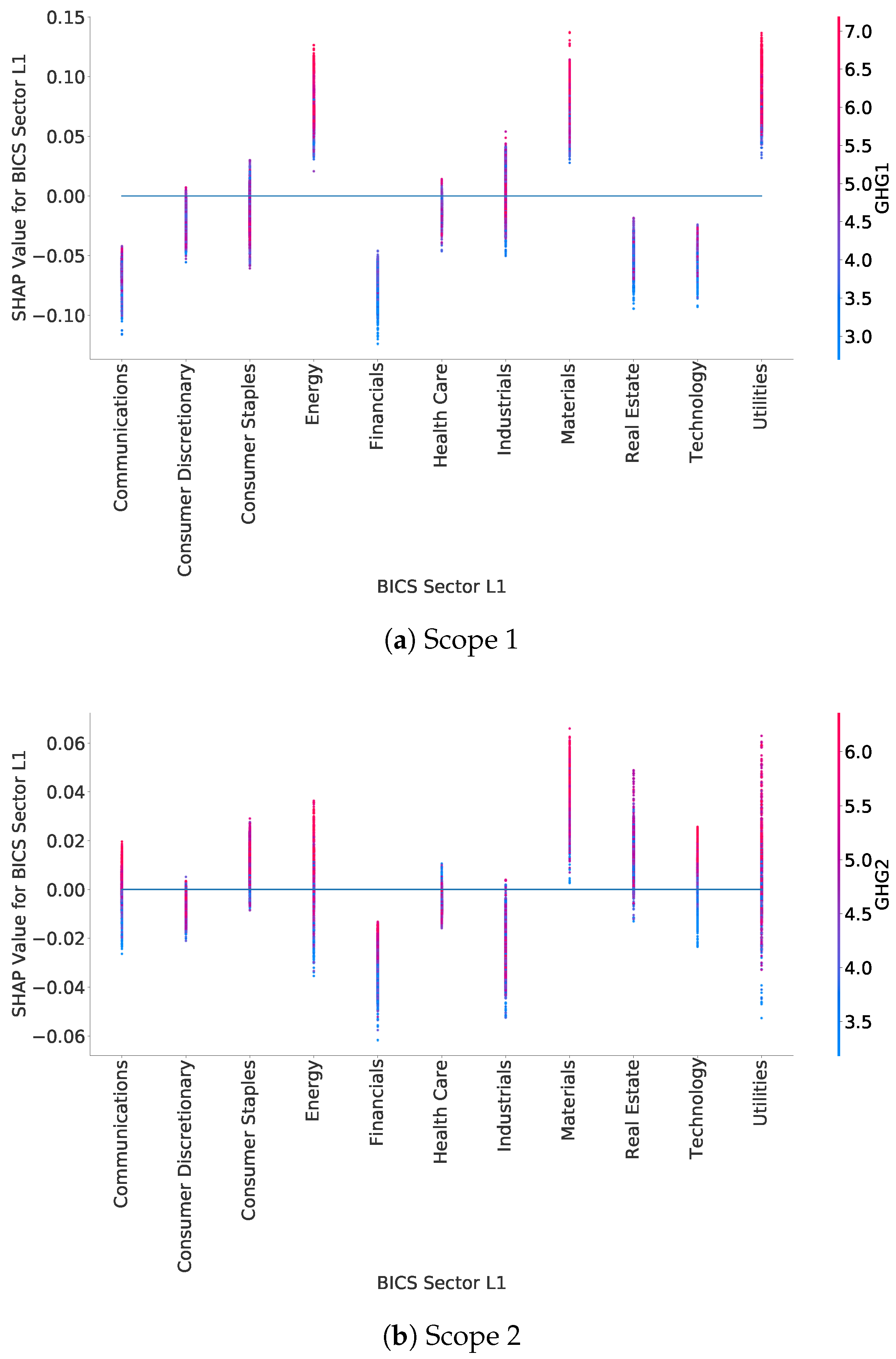
Figure 9 shows the distribution of SHAP values for the BICS Sector L1 feature, for each of the BICS Sector L1 sectors. This plot highlights in what sectors companies are more likely to have higher GHG emissions. For instance, for scope 1, SHAP values for all companies in the Energy and Materials sectors show an increase in the estimated emission (positive SHAP values). On the contrary, samples in the Financial sector have negative SHAP values, showing a decrease in the estimated emission.
This plot can be done for all categorical features, allowing us to understand the distribution of SHAP values according to each category, and then have a better interpretation of the model. In
Appendix B.2, an additional SHAP value plot for categorical features is provided, for further interpretation elements.
Plots in
Figure 9 highlight some clusters of SHAP values inside the distribution of BICS Sector L1 SHAP values per BICS Sector L1. These clusters show differences in the distribution of the initial data. Working on these clusters and removing the ones with too few samples could be a solution to improve the model by removing outliers and preventing overfitting. For instance, the distribution of SHAP values for the utility sector in scope 1 displays a cluster of SHAP values below 0.04 with few samples. These correspond to the years from 2012 to 2014 of a specific company for which the reported Energy Consumption is around 19 000 GWh, whereas the reported values for the same company from 2015 to 2020 are between 30 and 65 GWh. The removal of this cluster with very few samples allows for improving the quality of the training data by removing outliers. Similar studies on other sectors lead to the same results: for the Materials sector, it can lead to the removal of the only years a company did not report its Energy Consumption, for instance.
7.2.3. Data Polishing
This methodology should, however, be automated and applied systematically. A first implementation using the SHAP distribution for each BICS Sector L4 (Level 4 of granularity) was done. For each L4 sector, a hierarchical clustering algorithm is applied, separating clusters if their distance is above 0.04 in the SHAP values space, and removing clusters of data with an insufficient number of samples, i.e., less than 10. All these parameters were found using trial and error. For both scope 1 and scope 2, it leads to the removal of about respectively 11.5% and 5% of the training data, enabling an improvement in the global performance of the model. Results are presented in
Table 7, on average on the 5 different test sets: for both scopes, there is an average
RMSE decrease between 11% and 13%. It may come at the price of an increase of variability between results in the different test sets, especially for scope 1, as shown by the standard deviation of the RMSE metric in
Table 7a. As future work, studying more the impact of this methodology on both global and granular performances may lead to a more accurate and robust model.
8. Conclusions
To mitigate the fact that GHG emissions reporting and auditing are not yet compulsory for all companies and that methodologies of measurement and estimations are not unified, we proposed a machine-learning model to estimate non-reported company GHG emissions for scopes 1 and 2. The resulting model showed good out-of-sample performances when assessing it globally as well as good and balanced out-of-sample performances when assessing it per sector, country, and bucket of revenues. Comparing the obtained results to those of other providers, as of August 2022, we found our generated estimates to be available for a larger number of companies and more accurate.
In addition to its large coverage and accuracy, this model is also flexible, allowing for easy evolution of the input data as regulations evolve. It is also transparent, reproducible, and explainable: the methodology is described in this study extensively, and the implemented tools based on Shapley values allow us to understand the role played by each feature in the construction of the final output. We focused on some important interpretability elements, but many more interactions could have been studied: interaction between sectors, revenues, and the estimated GHG emission redoing the study done in this paper for each sector separately. These would give even more information on how the model is working and allow us to understand the specificities of GHG emissions per sector. Studying all these SHAP values interactions is beyond the scope of this study and could be the object of an entire future publication.
Future work to improve the model will first focus on gathering and including more training data from SMEs so that the coverage of the model is further improved. As it was stressed in this analysis, the used industry classification is critical: sometimes, companies operating in very different sectors in terms of GHG emissions can be grouped together. Gathering data about all the activities a company reports being active in, and working on, including this new and more precise industry classification in the model, will help in improving its accuracy. The data polishing method introduced in the last section of this study will also be developed with the goal of obtaining a more robust model. Future work on the interpretability of the model will focus on the performance improvement linked to the availability of the reported features. For instance, firms reporting energy consumption or production data without reporting their GHG emissions are the only beneficiaries of these particular features.


