Article

Research on Highway Self-Consistent Energy System Planning with Uncertain Wind and Photovoltaic Power Output

1
School of Control and Computer Engineering, North China Electric Power University, Beijing 102206, China
2
China Institute of Energy and Transportation Integrated Development, North China Electric Power University, Beijing 102206, China
3
State Key Laboratory of Rail Traffic Control and Safety, Beijing Jiaotong University, Beijing 100044, China
*
Author to whom correspondence should be addressed.
Sustainability 2023, 15(4), 3166; https://doi.org/10.3390/su15043166
Submission received: 2 December 2022 / Revised: 5 February 2023 / Accepted: 7 February 2023 / Published: 9 February 2023

Abstract

:
Highways are a critical consumer of energy. The integration of the highway and the energy system (ES) is a proven method towards carbon neutrality. The increasing energy demands of highway transportation infrastructure and the development of distributed energy and energy storage technologies drive the coupling between the highway system (HS) and the energy supply network, which is becoming tighter than ever before. Many scholars have explored the mode and path of integrated transportation and energy development. However, the energy and transportation systems’ coupling relationship and the collaborative planning scheme have not been thoroughly studied. Facing the increasing interconnection between transportation and energy networks, as well as addressing the demand for clean energy in highway transportation effectively, this paper proposes a highway self-consistent energy system (HSCES) planning model integrating uncertain wind and photovoltaic (PV) power output, so as to analyze the energy supply mode of the HS and determine the multi-energy capacity configuration of the self-consistent energy system (SCES). Firstly, the mathematical model related to each micro-generator of the SCES and the load aggregation scenario of the HS is established. Secondly, considering the uncertainty of renewable energy, this paper focuses on wind and PV power generation, and abatement technology, under uncertain conditions to ensure the best solution for reliability. Thirdly, taking the economy, reliability and the renewable energy utilization rate of the system into account, the system planning model is established under the condition of ensuring the system correlation constraints. Finally, the proposed method is validated using a section of the highway transportation system in western China. The results show that the hybrid energy storage planning scheme can cause the system’s renewable energy utilization rate to reach 99.61%, and the system’s power supply reliability to reach 99.74%. Therefore, it is necessary to carry out coordinated planning while considering the characteristics of the HS and the ES, which can minimize the planning cost of a HSCES, reduce the waste of wind and solar energy, and ensure the reliability of the power supply for the HS.

1. Introduction

In recent years, the coupling between internet technology and the energy system (ES) has been deepening, and the Energy Internet has gradually become a new form of energy industry [1,2]. As the primary sector for national economic development, intelligent transportation becomes the direction for the future of transportation system development [3]. Along with rapid economic and social growth in China, the demand for energy in the transportation sector is increasing yearly; whereas, energy supply is decreasing [4,5]. As an essential energy load, the transportation system has frequent interaction with and influence from the ES at the level of energy and information [6,7,8]. The ES is the energy carrier of the transportation system, while the transportation system is the driving object of the ES. Breaking the barrier of the isolated development of the existing ES and transportation system, and promoting deep integration between the energy and transportation systems, have become the research challenges and key issues that need to be solved by scholars at home and abroad.
In recent years, domestic and foreign researchers have achieved a lot in the application of renewable energy in the transportation sector [9,10,11]. References [12,13] reviews the current status of PV power generation and its comprehensive application to transportation, assesses the potential of PV power generation for highway transportation in China, and explores the feasibility of low-carbon and green transportation. Kim et al. [14] reasonably assess the wind energy resource potential of roads. The research establishes a set of evaluation methods, such as a spatial resolution sensitivity evaluation and a road proximity sensitivity assessment, which can maximize the use of wind energy resources while ensuring road safety, and provides some references for highway transportation wind energy utilization and microgrid planning. Zhang et al. [15], based on the analysis of energy consumption and the economy of urban transportation, constructs a system dynamics model to address highway system energy demand. This model overcomes the problem of inaccurate energy consumption prediction of the highway system, and provides a theoretical basis for highway system energy conservation, emission reduction and green transportation development. Although, the studies mentioned above have some guiding significance for evaluating transportation load demands and the potential of wind and PV power in transportation, those studies are limited to the assessment of the possibility of wind and PV renewable energy sources in transportation. The studies cited consider less how energy is stored and utilized in the case of the interaction between ESs and transportation systems.
The energy networks and transportation networks are all taking on the critical task of green and low-carbon transformation [16,17,18,19]. Developing clean energy and building green transportation is the key way to transform the energy network and transportation network into green, low-carbon versions. Therefore, the growth of energy and transportation has been combined, and many scholars have made certain progress in exploring the path to energy and transportation integration [20,21,22]. In terms of energy collection and storage by the transportation system, Wang et al. [23] proposed a highway energy collection and storage system by studying the laws of energy collection and storage under different traffic conditions. Through validation analysis, a strategy scheme for collecting and storing energy more accurately and efficiently was obtained; thus, the feasibility of highway traffic energy storage and utilization was verified. Wu et al. [24] constructed an integrated energy transportation system model with energy dispatch as the focus, renewable energy as the carrier, battery charging and switching stations as the medium, and the transportation system as the entity, creating the conditions for the integration of energy and transportation. Farahani et al. [25] proposed an integrated energy harvesting and transmission system for the clean energy utilization of carriers in transportation systems, which uses renewable energy to generate electricity and electrolysis to convert the remaining renewable energy into hydrogen to power hydrogen fuel–cell vehicles. The research created the conditions for a 100% renewable integrated energy transportation system. In terms of the form and development mode of energy and transportation integration, Yang et al. [26] described the synergy of energy and transportation convergence networks from a system interconnection perspective. They discussed the current status and potential future of energy transportation integration from the perspective of development trends, technologies and policies, and key technologies. He et al. [27] summarized the advantages of the integrated development of energy, transportation and information networks. Then, they established the energy transportation information complex network model and the energy transportation stochastic–type interaction mechanism, which effectively promoted renewable energy substitution for electrical energy in transportation systems. Huang et al. [28] proposed a long-term energy substitution planning model for the transportation system. By simulating the energy consumption demand and energy conservation potential in the transportation field of Guangdong–Hong Kong–Macao Greater Bay Area, the path to energy transformation of the transportation system was planned, which pointed out the direction for energy transformation of different transportation departments. Wei et al. [29] modeled the integration of energy and transportation systems based on the concept of an energy transportation convergence system. The energy allocation strategy of the transportation system was summarized by quantifying the operation state and equilibrium position of the electric power network in the transportation system. Both domestic and international research on the integration of energy and transportation emphasizes the integration concept and the possibility of integration strongly, but the coupling relationship, collaborative planning scheme and energy management strategy between the ES and the HS under the synergy analysis have not been studied deeply.
The rational allocation of the energy system is key to the planning and design of the HSCES [30]. The system structure, energy coupling mode and energy storage mode in the optimal allocation model have attracted the attention of many scholars. Pradhan et al. [31] proposed a new highway microgrid concept, which designed a grid-connected wind–solar power generation system on the highway system, transforming the transportation system from an energy consumer to an energy producer, reducing the operating costs of the highway transportation system, and promoting the development of green transportation. Doost et al. [32] proposed a charging–discharging strategy for the intelligent energy storage battery in order to minimize the dependence of the PV transportation microgrid on the main power grid. While reducing the peak power consumption of the power grid, the strategy also reduces the energy consumption of the transportation system. Liu et al. [33] integrated the wind–solar power highway microgrid into the main power grid, and proposed an adaptive control strategy for the highway microgrid system. This strategy rationally regulates the energy flow between the microgrid and the main power grid, and realizes the energy management of multiple highway microgrids under the grid connection mode. There are few studies on transportation microgrid systems, and the current research is limited to highway microgrids’ planning and energy management strategies with the primary power grid as support. In addition, the renewable energy connected to the microgrid is mainly single renewable energy, and the coupling effect of multi-energy complementation after hydrogen energy connection is rarely considered.
The highway load gathering scenario includes service areas, tunnels, bridges, toll stations, and equipment along the highway, etc., providing operational functions, such as lighting, monitoring, and communication. In this paper, we analyze the composition and influencing factors for energy consumption during highway operation, and propose an energy consumption measurement model applicable to highways based on existing energy consumption calculation methods. Meanwhile, we consider the coupling relationship between the SCES and the HS, and develop a multi-mode operation control strategy. Based on full consideration of the system power supply reliability and the renewable energy utilization rate, the optimal planning model of the HSCES integrating uncertain wind and PV power output is established to minimize the whole life–cycle annual value–cost of the system. Collaborative planning of distributed units, such as wind turbines, PV panels, batteries, and hydrogen storage systems, in the system is carried out to explore the potential interaction between the energy system and the transportation system. The simulation results in this paper verify the potential benefits and the necessity of collaborative planning between the ES and the HS in ensuring the system’s economic cost, energy utilization, and power supply reliability. As green transportation is the developing trend of the future, the planning method proposed in this paper can be used as a reference for the mode and results from the combination of renewable energy and transportation.
Relevant nomenclatures and units are defined in this paper, as shown in Table 1.

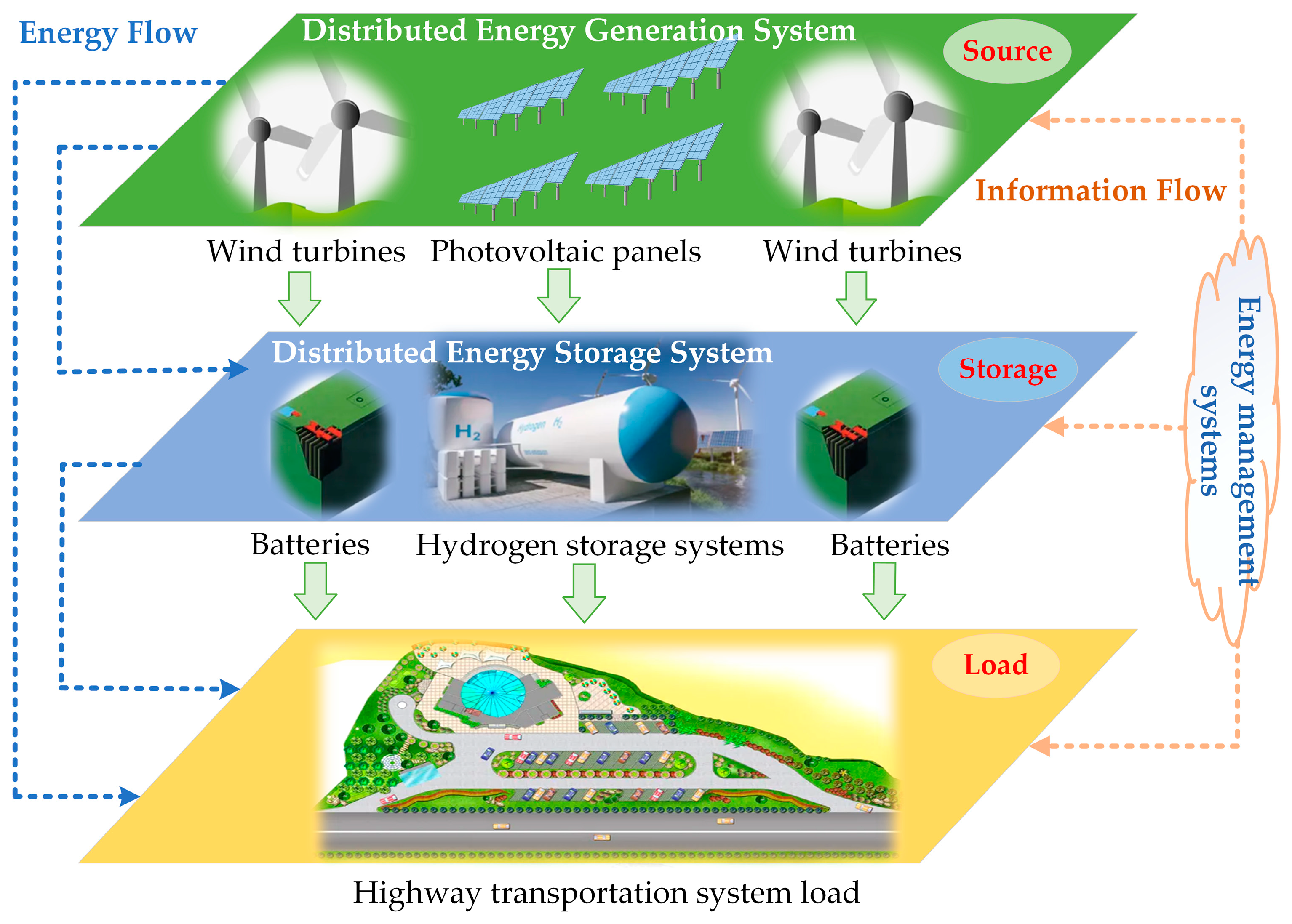
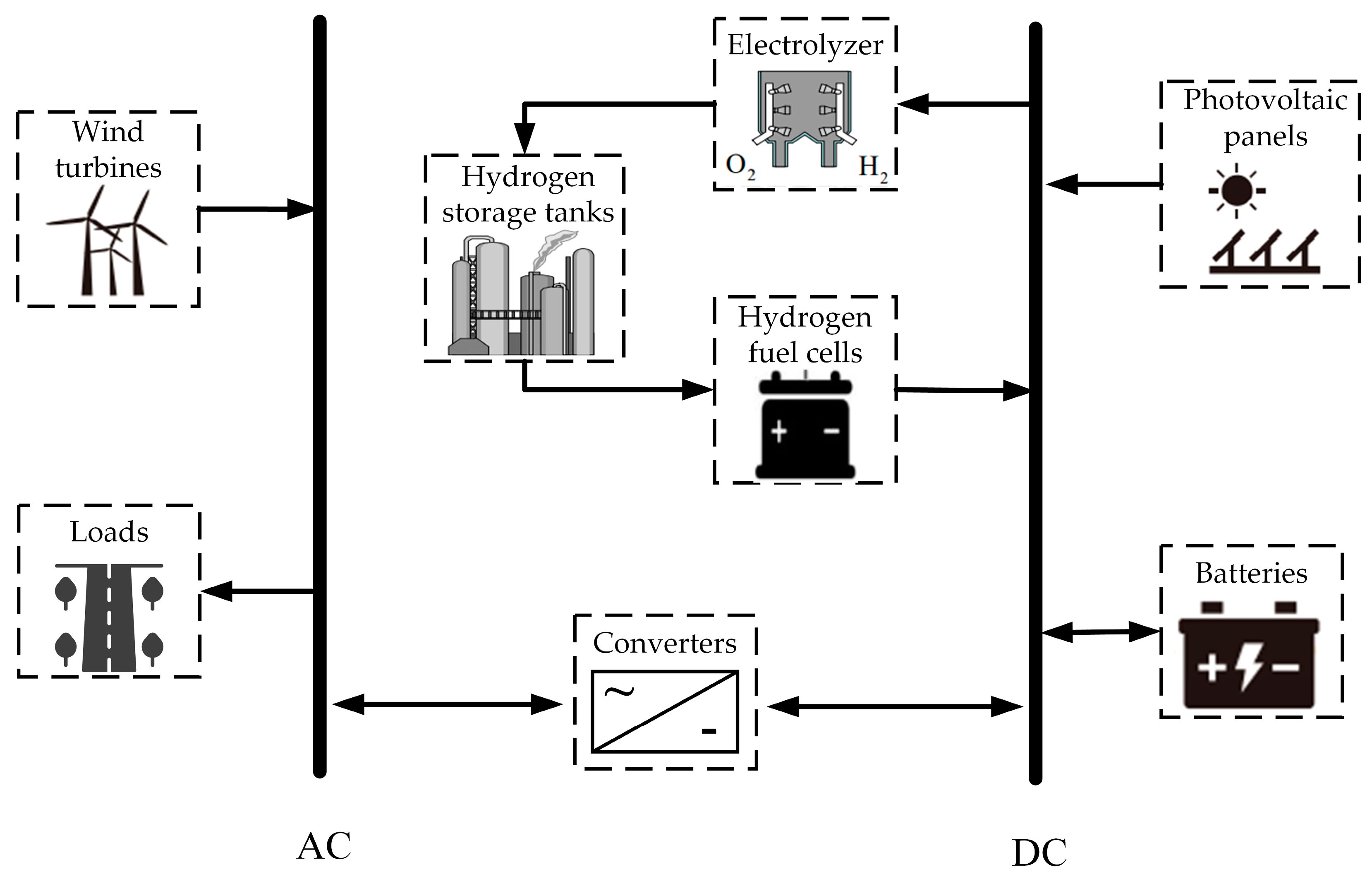
2. Architecture of Highway Self-Consistent Energy System

The term "microgrid" refers to a small-scale power production and distribution system made up of dispersed power sources, energy storage devices, energy conversion devices, monitoring and protection devices, and related loads [34]. Unlike traditional microgrids that require a large power grid and auxiliary energy supply equipment for support, we designed a "microgrid" specifically to meet the energy needs of highway transportation infrastructure, and generate energy from transportation infrastructure assets, as a "highway self-consistent energy system (HSCES)" to achieve clean energy use in the highway system (HS).

2.1. System Architecture

Highways serve as a practical and effective transportation infrastructure, and are crucial to industrialization and urbanization processes. The scale of China’s highway transportation infrastructure construction continues to expand, with electricity demand rising yearly. Through the optimal modification of the energy structure of the HS, an efficient technique can ensure that the energy need is met by clean energy.
The HSCES, which was located in the terminal area without a power network in Western China, shows the triple attribute of “source–storage–load”. On the basis of traditional energy supply, on the one hand, with the help of advanced power electronics technology and relying on renewable energy for power generation, the form-of-energy side changes into the form-of-power-supply side, and gradually adjusts the highway transportation infrastructure energy mode adapted to the energy transformation; thus, a new energy transport system structure with renewable energy as the primary energy supply has been formed in the “source–storage–load”. On the other hand, with the help of advanced information and electronic technology, the interconnection of energy information for all aspects of the generation, storage, distribution and use, and the flexible operation of the new the HS, can be realized.
The HSCES consists of renewable energy generation, electricity for highway transportation infrastructure, and hybrid energy storage equipment, as shown in Figure 1. This system can maximize the power generation potential of renewable energy, provide a clean power supply for highway transportation, and realize energy leveling with the help of an energy storage system, to form a new mode for the "source–storage–load" synergistic energy transportation system.
The architecture of the HSCES is shown in Figure 2. With abundant renewable energy in the western region of China, in order to achieve 100% renewable energy consumption and 100% zero-carbon power supply, distributed PV power generation and distributed wind power generation are adopted as energy supply modes in terms of the source side. On the grid side, due to the poor coverage of the grid in western China, there is basically no backbone transmission network, so it comes under the “Island Operation Mode”. As for the load side, the primary consideration for the HS service area, toll stations, bridges, tunnels and other infrastructure, is providing energy. On the energy storage side, considering the hybrid energy storage mode of electricity and hydrogen storage, the hydrogen storage system has characteristics including a wide operating range and fast power change rate, and is coupled with renewable energy; as such the utility model can effectively lessen the effects of renewable energy on the power grid and promote the absorption of renewable energy [34].

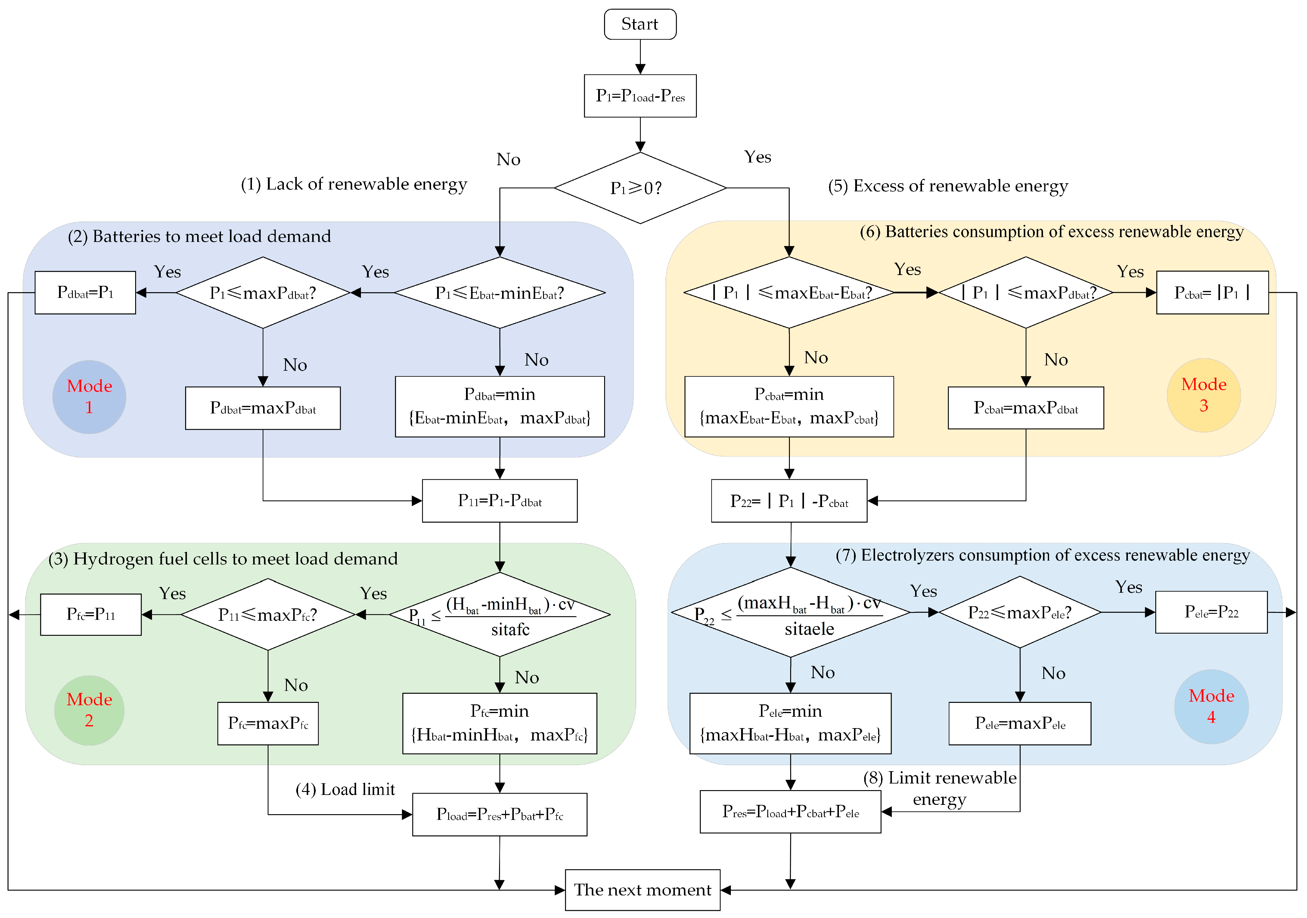
2.2. Control Strategy for System Operation

To maximize renewable energy consumption and ensure the reliability of the power supply in the HS, this paper proposes a control strategy for the HSCES, as shown in Figure 3. When the wind and PV output power are insufficient to satisfy the load requirements, the battery is first used to suppress the power fluctuation of the load and the renewable energy. When the battery cannot adjust the unbalanced power completely, the hydrogen storage system starts, and adjusts the remaining unbalanced power.
The detailed steps are as follows:
(1)
Start the system’s energy flow at a certain time. Firstly, the unbalanced power of the system is calculated. If the wind and PV output are insufficient to satisfy the load requirements, the system will enter Operation Mode 1. Otherwise, it will switch to Operation Mode 3;
(2)
Operation Mode 1: If the remaining battery power can meet the remaining load, and the remaining load is within the maximum discharge power limit of the battery, the battery can meet the remaining load; if the remaining battery power can satisfy the remaining load, but the remaining load exceeds the maximum discharge power limit of the battery, then the battery will discharge at the maximum power; if the remaining battery power cannot satisfy the remaining load, the discharge power of the battery takes the minimum value of both the remaining battery power and the maximum discharge power of the battery, at this point, the system calculates the imbalanced power and switches to Operation Mode 2;
(3)
Operation Mode 2: If the remaining hydrogen storage capacity of the hydrogen storage tank can satisfy the remaining loads, and the remaining loads are within the maximum hydrogen fuel cell output limit, the hydrogen storage system can satisfy the remaining load requirements; if the remaining hydrogen storage capacity of the hydrogen storage tank can satisfy the remaining load, but the remaining load exceeds the maximum output limit of the hydrogen fuel cell, the hydrogen fuel cell will output at the maximum power; if the remaining hydrogen storage capacity of the hydrogen storage tank cannot satisfy the remaining load, the output power of the hydrogen fuel cell takes the maximum output of the remaining hydrogen storage capacity and the maximum output power of the hydrogen fuel cell, enter step (6);
(4)
Operation Mode 3: If the maximum rechargeable capacity of the battery can absorb the excess renewable energy and it does not exceed the battery’s maximum allowable rechargeable power, then the battery absorbs the excess renewable energy output; if the maximum charge capacity of the battery can absorb the excess renewable energy, but the excess renewable energy output exceeds the maximum charge power limit of the battery, then the battery maintains the maximum charge power; if the maximum rechargeable capacity of the battery is unable to absorb the extra renewable energy, the battery’s charging power is equal to the lesser of its maximum rechargeable capacity and its maximum charging power, enter Operation Mode 4;
(5)
Operation Mode 4: If the excess renewable energy can be absorbed by the hydrogen storage system and its output is within the maximum output power limit of the electrolysis cell, then the hydrogen storage system can absorb the excess wind and PV output; if the hydrogen storage system can meet the remaining load, but the excess renewable energy output exceeds the electrolysis cell output power limit, then the electrolysis cell will maintain the maximum power output; if the hydrogen storage system cannot absorb the excess renewable energy, the actual output power of the electrolysis cell is the minimum value of both the electrolysis cell power consumed when the maximum hydrogen storage capacity is reached and the electrolysis cell reaches the maximum output power, enter step (6);
(6)
End the system’s energy flow at that moment and move on to the next.

3. Source–Storage–Load Triple Model of the HSCES

To reasonably evaluate the distributed clean energy output characteristics on the HSCES in western China and the energy demand of the HS, the demand models of distributed energy, distributed energy storage, and highway transportation load are as follows.

3.1. Distributed Energy Model

3.1.1. Wind Turbine Output Model

The power output curve of the device, turbine hub height and wind speed at the hub height are the primary determinants of a wind turbine’s output power [35], which can be expressed as:
P w t = { 0 S < S c i P r a S r a 3 S c i 3 S 3 P r a S r a 3 S c i 3 S c i 3 S c i S < S r a P r a S r a < S < S c o 0 S S c o
where: P r a is the rated power of the wind turbine (kW); S r a is the rated wind speed of the wind turbine (m/s); S is the actual wind speed of the wind turbine at the hub height (m/s); S c i is the cut-in wind speed of the wind turbine (m/s); S c o is the cut-out wind speed of the wind turbine (m/s).

3.1.2. PV Output Model

The output power of the PV array has an inevitable fluctuation and regularity, mainly affected by solar radiation intensity, temperature and other factors [36]. The PV array’s power output may indeed be stated as:
P p v = P s G ( φ , m , d , h ) 1000 G 0 [ 1 + θ T ( T T r e f ) ]
where: P s is the rated power of the PV array (kW); G ( φ , m , d , h ) is the solar radiation intensity at latitude φ , in the m month, d day, h hour (W/m2); G 0 is the standard solar radiation intensity, at 1 kW/m2; θ T is the power temperature coefficient of PV array [37]; T is the operating temperature of the PV array (°C); T r e f is the reference temperature for the PV arrays, at 25 °C.

3.2. Energy Storage System Model

3.2.1. Battery Charge and Discharge Model

The battery equipment of the HSCES can realize the time shift of energy. Generally, energy storage is performed when the energy supply is larger than the load requirements, and energy is released when the load requirements are larger than the energy supply. The operation model of the energy storage device considering self-discharge and charge-discharge power is shown in Equation (3) [38]:
E b a t t + 1 = ( 1 β ) E b a t t + η c b a t P c b a t t Δ t P c b a t t Δ t η d b a t
where: β is the self-discharge rate of the battery equipment; E b a t t is the whole electrical energy that is kept in the battery equipment at the time t (kWh), which takes into account the energy the battery has stored before, as well as the current net input, output power, and efficiency of the charge–discharge cycle; P c b a t t is the battery equipment charging power at time t (kW); P d b a t t is the battery equipment discharging power at time t (kW); η c b a t is the charge efficiency of the battery equipment; η d b a t is the discharge efficiency of the battery equipment; t is the sampling point at a certain time in the planning period, and the sampling period Δ t is 1 h.
The battery state of charge (SOC) model is as follows:
S O C ( t ) = { ( 1 β ) S O C ( t 1 ) + P c b a t ( t ) Δ t η c b a t C b a t ( 1 β ) S O C ( t 1 ) + P d b a t ( t ) Δ t η d b a t C b a t
where C b a t is the rated capacity of the battery (kWh).

3.2.2. Hydrogen Power Generation System Model

Hydrogen power generation system refers to the production of hydrogen through environmently friendly and recyclable energy, and energy conversion in different carriers, such as hydrogen fuel cell systems that generate power to achieve peak regulation and frequency regulation. Compared with other energy storage technologies, hydrogen energy storage has the characteristics of a long shelf-life and high-energy density. The three-terminal model of production–storage–use is as follows:
(1)
Electrolytic hydrogen production equipment output model
At the core of electrolytic hydrogen equipment, electrolysis cells electrolyze water into hydrogen and oxygen [39]. This paper assumes that the electrolysis cell is insulated and the electrolysis cell conversion efficiency remains constant during its operation [40]. The output power of the electrolysis cell is:
P ele = η ele P ele i n
where: P ele i n is the electrolysis cell input power (kW); η ele is the electrolysis cell efficiency.
(2)
Remaining capacity model of the hydrogen storage tank
The hydrogen storage tank links hydrogen production and hydrogen consumption. It can store the hydrogen generated by electrolysis from the water in the electrolysis cell and provide hydrogen for hydrogen fuel cell power generation. The energy storage model of the hydrogen storage tank is as follows:
E Q h 2 ( t ) = E Q h 2 ( t 1 ) + η e l e P e l e i n ( t ) Δ t P f c ( t ) Δ t η f c
where: P f c ( t ) is the output power of the hydrogen fuel cell at the time t (kW); η f c is the efficiency of the hydrogen fuel cell.
(3)
Hydrogen to electricity equipment output model
There are two main ways to utilize hydrogen energy, which are through a hydrogen fuel cell and through a hydrogen-fueled internal combustion engine. Table 2 provides comparative analysis of the two options.
As the table shows, hydrogen fuel cells have the advantages of producing no NOx emissions and having high conversion efficiency when compared with hydrogen-fueled internal combustion engines, while requiring a smaller hydrogen storage tank, which is more suitable for the practical needs of the HSCES. Therefore, we adopted the hydrogen fuel cell as the hydrogen–electricity equipment.
In this paper, when a solid oxide fuel cell is used, the output power of the hydrogen fuel cell will be:
P f c = η fc P f c i n
where P f c i n is the input power of the hydrogen storage tank to hydrogen fuel cell (kW).

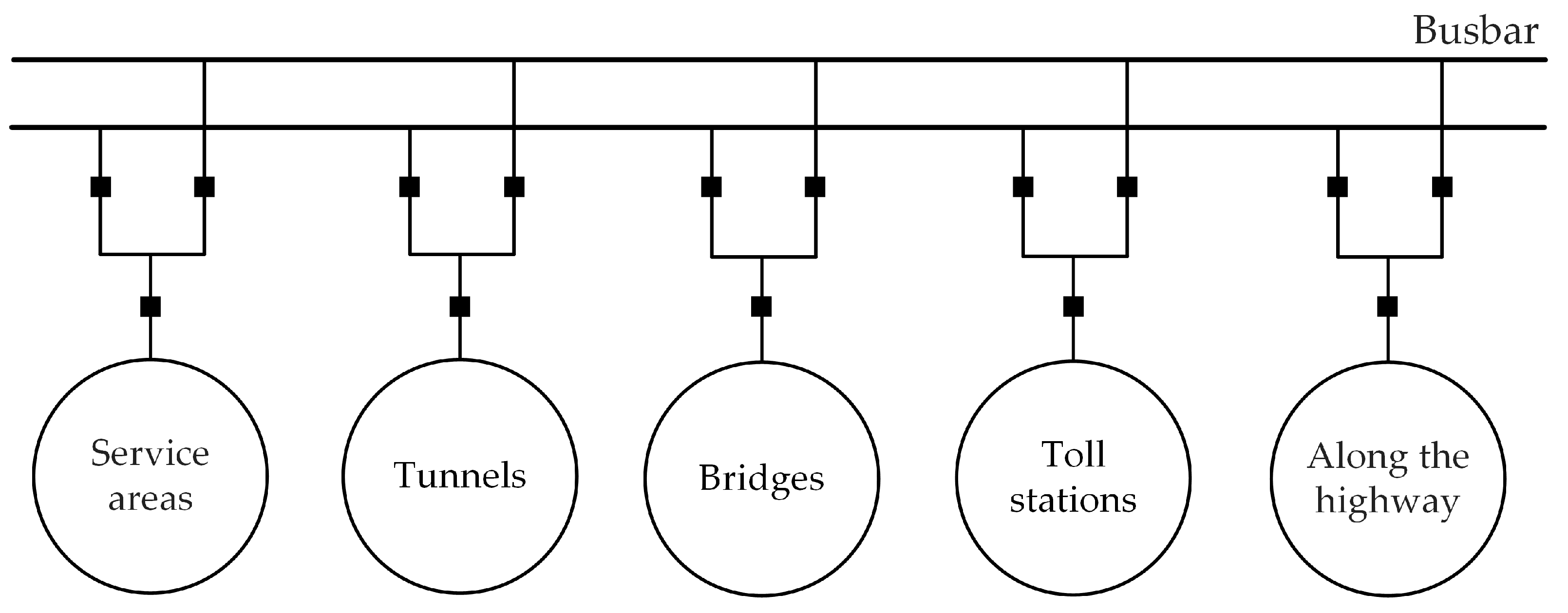
3.3. Highway Transportation Load Model

The energy consumption of the HSCES during operation corresponds with the service area, tunnel, bridge, toll station and other ancillary facilities along the road, etc., to meet the requirements of the HS monitoring, lighting, information control, management, service and other operational functions. The correlation between function–carrier–energy consumption of the HS is shown in Figure 4.
The HSCES proposed in this paper is mainly designed to meet the energy supply of highway transportation infrastructure in the gridless areas of western China, which has neither a large grid to provide power support nor auxiliary energy supply equipment to provide electrical energy. Therefore, the HS load is entirely supplied by the energy generation of the highway transportation infrastructure assets. Among them, service areas, tunnels, and equipment along the highways are both the electrical energy supply side and the energy-consuming side. In contrast, bridges and tunnels cannot use asset-based energy generation and can only be used as energy-consuming units. Each loading unit of the system is connected to the same set of busbars for energy interaction; the topology diagram is shown in Figure 5.
We analyze the energy demand of highway infrastructure for energy consumption. The infrastructure–energy–consumption measurement model is as follows:
Q = Q F + Q S + Q B + Q T + Q R
where: Q is the energy utilized by all infrastructures (kWh); Q F is the energy utilized by the service areas (kWh); Q S is the energy utilized by the tunnels (kWh); Q B is the energy utilized by the bridges (kWh); Q T is the energy utilized by the toll stations (kWh); Q R is the energy utilized by the equipment along the highway (kWh).

3.3.1. Service Area Energy Consumption

The energy utilized by the service areas is primarily the energy consumption by restaurants, supermarkets, rooms, office areas, gas stations, etc. The energy consumption of service areas is calculated using the general analogy technique, since the energy-consuming equipment of gas stations and restaurants is typically locked and thus, challenging to count. On the basis of the average power consumption statistics of other service areas, it can be calculated using the accumulating and summing data from the hourly power consumption in the service area, the specific formula is as follows:
Q F = t = 1 8760 ( i = 1 m q i 1 ( t ) + j = 1 n q j 2 ( t ) )
where: q i 1 ( t ) is the energy utilized by the i th service area for one hour (kWh); q j 2 ( t ) is the energy consumption of the j th parking area for one hour (kWh); m and n are the number of service areas and parking areas of the HS, respectively.

3.3.2. Tunnel Energy Consumption

Tunnels on highways need to be equipped with ventilation, lighting, and monitoring and communication systems to ensure transportation safety. According to reference [8], tunnel energy consumption mainly includes the energy consumption of the equipment inside the tunnel and the equipment at the entrance and exit to the tunnel. The energy consumption model is as follows:
Q S = s = 1 n ( P s 1 T s 1 L S L s 1 + n 1 n S P s 2 T s 2 )
where: P s 1 is the rated power of the equipment inside the tunnel (kW); L s 1 is the equipment spacing (m); T s 1 is the working time of the equipment inside the tunnel (h); L S is the total length of the tunnel (m); n 1 is the number of pieces of equipment at each tunnel entrance and exit; n S is the total number of tunnels.; P s 2 is the rated power of the equipment at each tunnel entrance and exit (kW); T s 2 is the working time of the equipment at each tunnel entrance and exit (h).

3.3.3. Bridge Energy Consumption

There are various types of electrical equipment around bridges that ensure the safety of transportation. Bridges on highways need to be equipped with lighting, monitoring, detection equipment and other systems. According to reference [8], a bridge with a length of L kilometers usually requires the number of monitoring and detection equipment to be ( L 1 ) , and the bridge lighting system load is generally 15.98 kW/km. Therefore, the bridge energy consumption model is as follows:
Q B = P b 1 T b 1 L B + P b 2 T b 2 ( L B 1 )
where: P b 1 is the load coefficient of the bridge lighting system, at 15.98 kW/km, T b 1 is the working time of the lighting system (h); L B is the total length of the bridge (km); P b 2 is the rated power of the monitoring and detection equipment (kW); T b 2 is the working time of the monitoring and detection equipment (h).

3.3.4. Toll Station Energy Consumption

The primary energy consumption of the highway toll station comes from the toll collection system, monitoring system, lighting system and management office. According to reference [8], the toll station model is as follows:
Q T = P t 1 T t 1 n t
where: P t 1 is the load of the toll station, at 0.04 kW; T t 1 is the operation time of toll station (h); n t is the total number of toll stations.

3.3.5. The Energy Consumption of Equipment along the Highway

The vehicle detector and emergency telephone are the leading energy-consuming equipment along the highway. According to the highway mainline monitoring and communication needs and practical experience, ( L r 1 ) vehicle detectors and 2 ( L r 1 ) emergency telephones are required for the expressway at a length of L kilometers. The energy consumption model is as follows:
Q R = T r ( L r 1 ) ( 2 P d + P c )
where: L r is the length of the entire highway (km), P c is the power of vehicle monitoring devices (kW); P d is the power of emergency phones (kW); T r is the operation time of the highway (h).

3.4. Multi-Scenario Uncertain Wind and Light Output Model

As the accuracy of renewable energy power prediction keeps step with the refinement of the prediction scale, wind and PV power have strong volatility. Based on multi-scenario generation technology, this paper promotes modeling analysis. The specific model is as follows:
P i , m , t F C = P i , t F C ( 1 + ξ i ( R i , t λ ) )
where: P i , m , t F C is the power prediction for a typical scenario m in season at the time t (kW), i { 0 , 1 } , when i is 0, P i , m , t F C indicates the power prediction of the wind turbines, when i is 1, P i , m , t F C indicates the power prediction of the PV units (kW); P i , t F C is the power value at time t based on the historical power prediction (kW); ξ i is the percentage of the prediction error threshold; R i , t is a random number that follows a specific distribution, such as Weibull distribution, Beta distribution and normal distribution; λ is a random distribution correction factor.
PV output power prediction errors generally obey the Beta distribution [41], whose probability distribution is shown below:
f ( R j , t ) = N d R j , t α 1 ( 1 R j , t ) β 1
Wind power forecast errors are better characterized by the Weibull distribution [42,43]. The probability distribution is shown below:
{ f ( v ) = ( k c ) ( v c ) k 1 exp ( v c ) k k = ( σ v ¯ ) 1.086 c = v ¯ Γ ( 1 + 1 / k )
where: α and β are the shape and scale parameters of the Beta distribution, respectively; N d is the normalization factor; c and k are the shape and scale parameters of the Weibull distribution, respectively; σ is the standard deviation; Γ ( 1 + 1 / k ) is the Gamma function; v ¯ is the average wind speed (m/s).
Latin hypercube sampling is a multi-dimensional stratified sampling method, which can produce more evenly distributed sample points and is more efficient than random sampling [44]. Based on the above prediction model, this paper performs multi-scenario generation based on the Latin hypercube sampling technique. Therefore, according to the historical data of meteorological information and the prediction model based on Formula (14), when wind power is subject to Weibull distribution and photovoltaic technologies are subject to beta distribution, the multi-scenario set of wind power and photovoltaic output can be predicted. The main steps are to:
(1)
Equalize the probability distribution into n probability intervals, during a typical day of each season, n is 24.
(2)
Take the random number in each probability interval as the sampling point, and the equal probability independent sampling at each interval. The probability of each interval is expressed as:
p i n = p ( x i n S i n )
where: p i n is the sampling probability of the n t h interval of variable i ; and where p i n = 1 ; x i n is the sample of the n th interval of variable i ; S i n is the threshold value of the n t h interval of variable i .
(3)
Transform the probability distribution function inversely to obtain the sample value of the sampling point. The sample value corresponding to each subinterval is:
x i = f x i 1 ( S i n )
where: x i is the sample value corresponding to each subinterval; f x i 1 ( ) is the inverse of the probability distribution function f ( ) .
Given that the generation of a large number of scenarios will increase the burden of solving operations, this paper adopts the simultaneous back substitution method for scenario reduction. The reduced set of typical scenarios can reflect the probability distribution of the original set of scenarios. The main steps are to:
(1)
Calculate the closest scenario for each scenario x i .
{ D i = min ( λ i d ( x a , x b ) ) j = 1 , 2 , , n s o , j i
where: D i is the probability distance to the scenario x i ; λ i is the probability of scenario x i ; d ( x a , x b ) is the Euclidean distance between scenarios x i and x j ; n s o is the initial number of scenarios.
(2)
Identify the scenarios x i that need to be deleted.
D min = min 1 , 2 , , n s o ( λ i D i )
where: D min is the closest probability distance to the scenario x i .
(3)
Delete the above scenario, and add the probability of deleting the scenario to the probability of the scenario closest to it, so as to ensure the sum of the probabilities is 1. At this time, the probability is:
λ j = λ j λ i
(4)
Repeat the above steps until the number of remaining scenarios reach the set value.
After the above generation and reduction scenarios, the final number of typical scenarios for wind power and PV are n W T and n P V , respectively. Finally, the probable number of combined typical scenarios and the corresponding combined typical scenarios are:
n s = n W T n P V
{ λ s = λ W T λ P V S = 1 , 2 , , n s
where λ W T , λ P V are the probabilities corresponding to wind and PV scenarios, respectively.

4. Optimal Planning Model for the HSCES

System operators often want to rationally configure distributed power to reduce construction costs, as much as possible, while increasing internal revenue. On the basis of meeting the "spontaneous self-use" of local load, the greater the generation capacity of distributed power generation and the greater the income of system operators, the greater the construction costs of the system. How to assign system capacity to increase the economy and reliability of system operation is the central concern of the HSCES planning.

4.1. Objective Function

The life–cycle cost (LCC), maintaining the initial capital cost (ICC), and the operation and maintenance costs (OMCs) of the system, are the major components of the objective function and are converted into the equivalent annual cost (EAC). Meanwhile, the power supply reliability and renewable energy utilization rate of the system are considered.

4.1.1. Equivalent Annual Cost

Reducing the comprehensive annual cost is the operators’ goal during the HSCES planning, so the system payment function is established based on the minimum average annual payment cost of the system, as shown in Formula (24). Among them, the number of wind turbines, photovoltaics, storage batteries and hydrogen storage systems are the decision variables that need to be planned.
C N = C i n i t i a l + C o m
where: C i n i t i a l is the equivalent annual investment cost (EAIC) of the system micro-generator (¥); C o m is the equivalent annual operation and maintenance costs (EAOMCs) of the system micro-generator (¥).
(1)
EAIC
The system’s EAIC is the total of the equivalent annual ICC of each micro-generator, which is calculated as the equation:
C i n i t i a l = C i n i t i a l P V n 1 + C i n i t i a l W T n 2 + C i n i t i a l b a t n 3 + C i n i t i a l e l e n 4 + C i n i t i a l Q h 2 n 5 + C i n i t i a l f c n 6
where: C i n i t i a l P V , C i n i t i a l W T , C i n i t i a l b a t , C i n i t i a l e l e , C i n i t i a l Q h 2 and C i n i t i a l f c are the EAIC of the PVs, wind turbines, batteries, electrolysis cells, hydrogen storage tanks and hydrogen fuel cells (¥), respectively; n k ( k = 1 ~ 6 ) is the service life of each micro-generator. Each component is calculated as follows:
C i n i t i a l m = t = 1 8760 m = 1 6 N m P m U m r ( 1 + r ) L m r ( 1 + r ) L m 1
where: N m is the number of installations of each micro-generator in the system; P m is the rated output power of each micro-generator (kW); U m is the investment cost per unit of the power rating in each micro-generator (¥); L m is the service life of each micro-generator (year); r is the funding discount rate, at 0.04.
(2)
EAOMCs
The EAOMCs are the sum of the EAOMC of each micro-generator. They are calculated as the equation:
C o m = t = 1 8760 m = 1 6 N m P m M m
where M m is the micro-generator unit power operation and maintenance costs.

4.1.2. System Power Supply Reliability

The System power supply reliability refers to the ratio between the amount of power supplied to the HS and the actual load demand in a year. If the power supply time required by the HS in a year is 8760 h, the calculation formula of the annual average power supply reliability index of the system is:
A S A I = t = 1 8760 Q ( t ) t = 1 8760 Q l ( t ) t = 1 8760 Q ( t )
where: A S A I is the annual average power supply reliability index of the system (%); Q ( t ) is the load requirements of the system at time t (kWh); Q l ( t ) is the insufficient power at the time t (kWh).

4.1.3. Renewable Energy Utilization Rate

The renewable energy utilization rate can effectively measure the utilization of renewable energy generation in the system. The annual average renewable energy utilization rate of the system can be expressed as:
U r e n = t = 1 8760 E r e n t E e x c e s s t E r e n t
where: U r e n is the renewable energy utilization rate (%); E r e n is the wind and PV power generation (kW); E e x c e s s is the abandoned wind and PV capacity (kW).

4.2. Constraints

The planning model in this paper mainly considers the constraints of each micro-generator output, battery charging and discharging, hydrogen power generation system and system power balance.

4.2.1. Micro-Generator Constraints

The constraints related to wind and light output are:
(1)
Wind power output constraint:
0 P w t ( t ) N w t p w t ( t )
where p w t ( i ) is the power output of a wind turbine at the time t (kW).
(2)
PV power output constraint:
0 P p v ( t ) N p v p p v ( t )
where p p v ( i ) is the power output of a PV panel at the time t (kW).

4.2.2. Battery Charging and Discharging Constraints

The relevant constraints for the battery are:
(1)
Battery charge state constraint:
S O C min S O C ( t ) S O C max
where S O C min and S O C max are the lower and upper limits of the battery charge state, at 0.1 and 0.9, respectively.
(2)
Battery discharge power constraint:
0 P d b a t ( t ) N b a t P m a x d 1
where P m a x d 1 is the maximum discharge power of a battery (kW).
(3)
Battery charging power constraint:
0 P c b a t ( t ) N b a t P m a x c 1
where P m a x c 1 is the maximum charge power of a battery (kW).

4.2.3. Constraints Related to the Production–Storage–Use of the Hydrogen Energy Generation System

Constraints related to the production–storage–use of hydrogen energy generation systems are:
(1)
Electrolysis cell output constraint
0 P e l e ( t ) N e l e P m a x e l e 1
where P m a x e l e 1 is the maximum output of a single electrolysis cell (kW).
(2)
Hydrogen fuel cell output constraint
0 P f c ( t ) N f c P m a x f c 1
where P m a x f c 1 is the maximum power output of a single hydrogen fuel cell (kW).
(3)
Hydrogen storage tank capacity state constraint
S O C m i n H 2 S O C h 2 ( t ) S O C m a x H 2
where S O C m i n H 2 and S O C m a x H 2 are the lower and upper limits of the hydrogen storage tank capacity state, respectively, which are set at 0.05 and 0.95.
(4)
Hydrogen storage tank capacity constraint
0 Qh 2 N Qh 2 Q m a x H 2
where Q m a x H 2 is the maximum capacity of a hydrogen storage tank (kWh).
(5)
Hydrogen storage tank intake constraint
N h 2 c ( t ) = S e l e P e l e ( t ) c v
where: S e l e is the total efficiency of the electrolysis cell and the intermediary-pressure compressor, which is set at 0.6 [45]; c v is the calorific value of hydrogen, which is set at 39 kWh/kg.
(6)
Hydrogen storage tank discharge constraint
N h 2 d ( t ) = S f c P f c ( t ) c v
where S f c is the conversion efficiency of the hydrogen fuel cell, which is set at 0.6.

4.2.4. Power Balance Constraint

The system power balance constraint is:
P w t ( t ) + P p v ( t ) + P d b a t ( t ) + P f c ( t ) = P L o a d ( t ) + P b c ( t ) + P e l e ( t )
where P L o a d ( t ) is the system load power at the time t (kW).

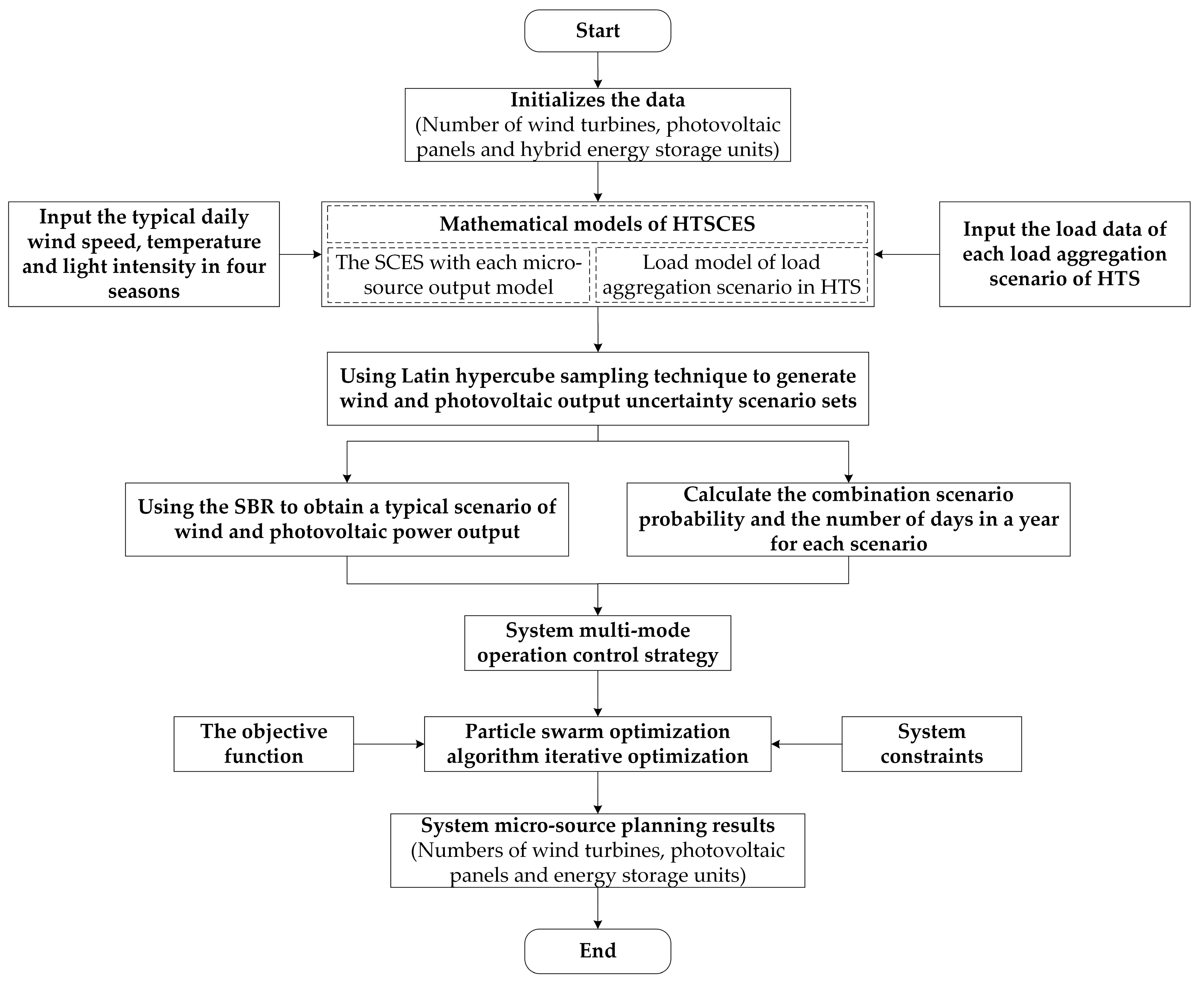
5. System Planning Model Solving Process

This paper emphasizes the optimal capacity planning of the HSCES using the particle swarm optimization (PSO) technique. The solution idea is to:
Initialize the configuration data for wind turbines, PV panels, hybrid energy storage units, etc.; as for system optimization variables, we set the following values: N P V is the number of PV panels, N W T is the number of wind turbines, N b a t is the number of batteries, N e l e is the number of electrolytic cells, N Q h 2 is the number of hydrogen storage tanks, and N f c is the number of hydrogen fuel cells.
(1)
Input the typical weather information (wind speed, temperature and light intensity) for the four seasons into the SCES and the load data of every load gathering scenario in the HS;
(2)
The Latin hypercube sampling technique is employed to produce the usual daily unpredictable wind and the PV output scenario sets for each season;
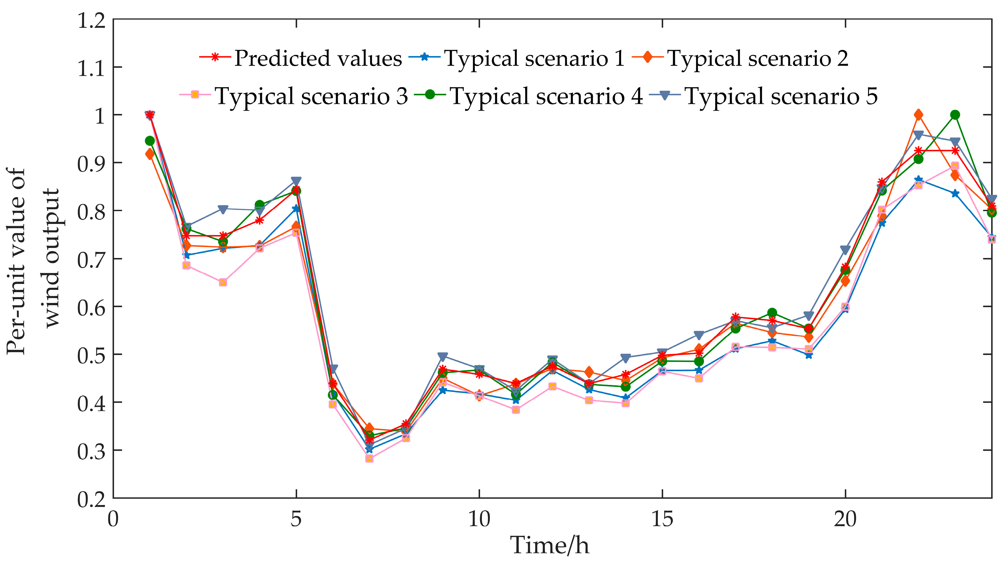
(3)
In order to conveniently handle the issue, the simultaneous backward reduction (SBR) method is used to obtain the typical scenarios and the occurrence probability of each scenario, as well as the number of days in each scenario in a year;
(4)
Formulas (22), (26) and (27) are used as the fitness function of the algorithm, and Formulas (28)–(39) are used as the constraint for each part of the system to construct the optimization model of the HSCES;
(5)
The optimal power capacity configuration of the HSCES under the operation control strategy is searched by the PSO algorithm until the optimal planning result of the system is obtained. The solution flow chart is shown in Figure 6.

6. Case Study

6.1. Problem Description

In this paper, our problems stem from the need for clean energy on the highways in western China. Using the G6 Beijing–Lhasa Expressway at the Golmud to Lhasa section, during the planning and construction process, our mathematical model and planning method have been applied in practice. We take the data on wind speed, light intensity, temperature and various load aggregation scenarios of the highway as the system input. According to the literature [8] and locally measured data, typical weather information for the four seasons is shown in Figure 7: the average daily wind speed was 8.10 m/s, the average daily light intensity was 146.67 W/m2, and the average daily temperature was 14.64 °C. The time by time superimposed load data for the highway load aggregation scenarios are shown in Figure 8: the average daily load was 858.13 kWh in a year, with the peak load appearing in summer and winter, and the load in spring and autumn being relatively low; in a day, the load fluctuation is slight, but the overall daytime load is higher than in the night.
To verify the advisability of the provided HSCES planning approach, the following simulation schemes are set up:
Scheme 1: Wind and solar energy, as the energy input of the HSCES, provide energy for various load gathering scenarios for highway transportation. On the energy storage side, only use the battery for power regulation and storage of the excess energy.
Scheme 2: Wind and solar energy, as the energy input of the HSCES, provide energy for various load gathering scenarios for highway transportation. On the energy storage side, the hydrogen storage system takes the place of the battery for power regulation and storage of the excess energy.
Scheme 3: Wind and solar energy, as the energy input of the HSCES, provide energy for various load gathering scenarios for highway transportation. On the energy storage side, the hybrid energy storage mode of the battery and hydrogen storage system is used for power regulation and excess energy storage.
Table 3 lists the primary equipment-related parameters available for selection in the HSCES planning model [46,47].

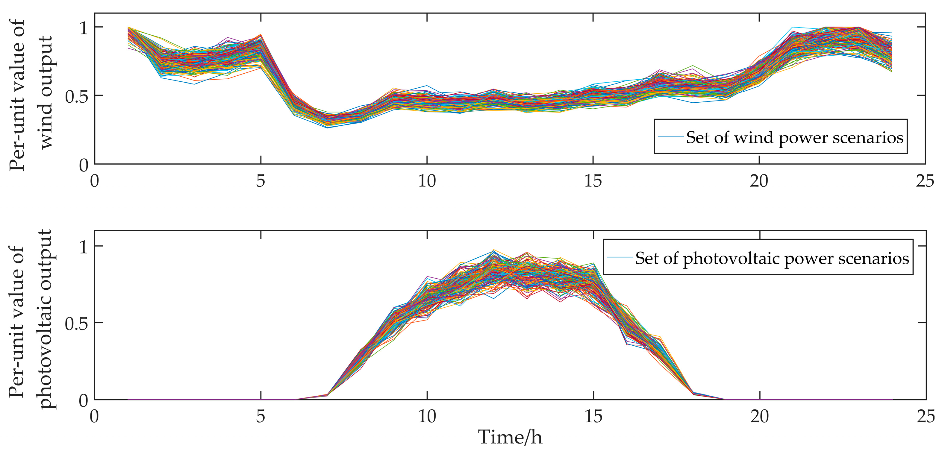
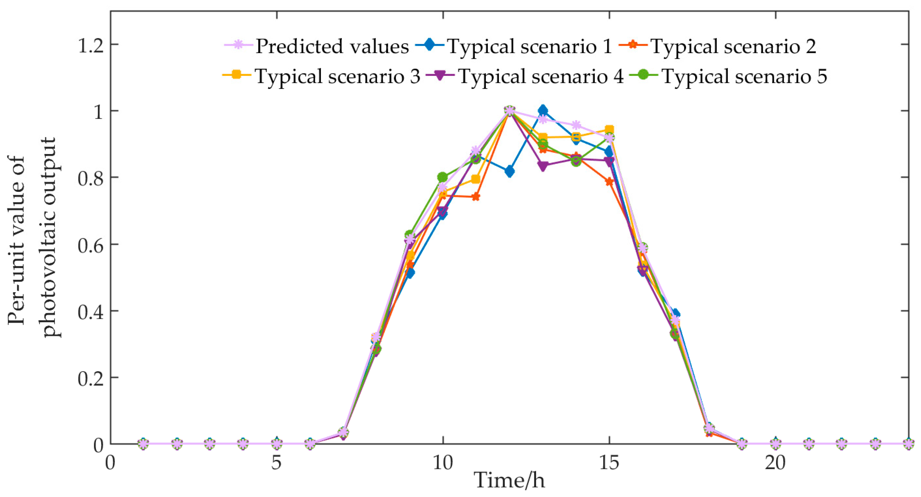
6.2. Analysis of Uncertain Wind and PV Output Scenarios

The generation and reduction of uncertain wind and PV output scenarios are typical occurrences in summer. Based on wind and PV forecast data, intra-day random scenarios are generated according to Formulas (14)–(16), and the Latin hypercube sampling technique as shown in Figure 9. Relative errors for wind and PV were set at 15% and 20%, respectively. The random scenario is reduced by using the SBR method. The number of typical scenarios for wind and PV is five separately, and the final combined typical scenario number is 25. The typical scenarios for wind and PV are shown in Figure 10 and Figure 11.
The typical scenario probabilities of wind and PV are shown in Table 4, and the combined scenario probabilities are shown in Table 5.

6.3. Convergence Analysis of the Algorithm

To evaluate the effectiveness of global search and convergence of the PSO algorithm for the HSCES planning model, 50 simulation experiments were carried out for the three schemes. Minimizing the impact of random factors, the number of populations is 60, and the maximum number of iterations is 400. Table 6 shows the PSO algorithm simulation results for three experimental design schemes of the HSCES planning model (Annual combined costs/10,000 CNY).
In Table 6, the variances of the three experimental design schemes were 1.3, 1.7, and 2.6, respectively. Moreover, because the system complexity of the three experimental design schemes is increasing step–by–step, the variance of scheme 3 is slightly larger than that of schemes 1 and 2. However, overall, the simulation results of the three experimental designs are kept within a narrow fluctuation range. The results show that the PSO algorithm has good convergence and global search ability for the micro-generator planning model of the HSCES.

6.4. Analysis of Micro-Generator Planning Results

According to the system control strategy shown in Figure 3 and the system parameters shown in Table 3, it is necessary to use the PSO algorithm to solve those three kinds of experimental design schemes for the HSCES. The results of the micro-generator planning are shown in Table 7. The simulation results of each system economy, renewable energy abandonment rate (REAR), and power outage rate (POR) are shown in Table 8. The analysis of various indexes under different experimental design schemes can provide some scientific basis for the investment decision-making for the HSCES and the realization of HSCES projects.
Compared with the single energy storage plan in scheme 1 and scheme 2, the hybrid energy storage plan in scheme 3 performs a more flexible configuration capacity for each micro-generator; at the same time, the micro-generator supply configuration of the system can be relatively reduced, and further lead to a substantial reduction in the number of energy storage system configurations. In contrast to schemes 1 and 2, the combined costs are reduced by 2.72% and 6.56%, respectively. At the same time, the desertion rate for renewable energy by the system is decreased, and the power supply reliability of the system is increased.
Specifically, when compared to scheme 1, scheme 3 absorbs excess electric energy by configuring several electrolytic cells and storing them in the hydrogen storage tanks. During high-load periods, the shortage is replenished by the output of the hydrogen fuel cell and by significantly reducing the number of battery configurations. Though relatively high in EAICs and EAOMCs, scheme 3 ensures the renewable energy utilization and reliability of the system, and improves customer satisfaction, while reducing penalty costs and making the system’s combined costs the lowest. When compared with scheme 2, scheme 3 can achieve a better time translation effect by using hybrid energy storage, which reduces the number of micro-generator supply configurations. At the same time, it is economical to use batteries to replace some of the more expensive hydrogen storage systems.

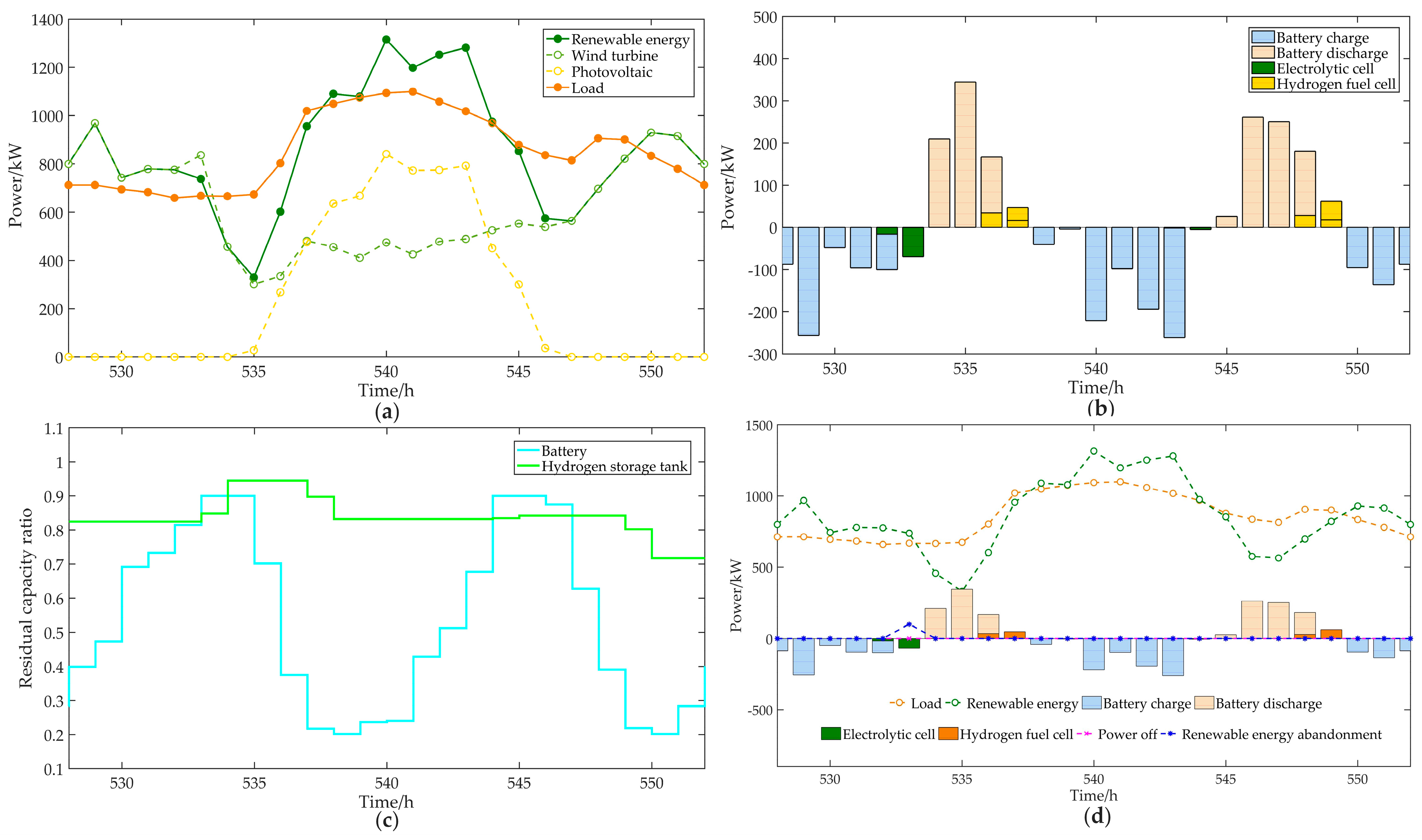
6.5. Analysis of the Actual Operation Effect of the System

Figure 12 shows the simulation results of scenario 23, which represents the highest probability in one year, and describes the actual operation effect of the system under the optimal planning strategy more intuitively.
As seen in Figure 12, the wind power output of the system is mainly concentrated at night, and the PV output only appears in the daytime. Wind power and PV have good complementarity. During the night hours from 528 to 533 and 550 to 552, the wind power production of the system is larger than the load. At this time, the battery and electrolysis cell in the hybrid energy storage system absorb excess wind power, and the remaining capacity ratio of the hybrid energy storage system increases correspondingly. During the daytime, from 534 to 537, the wind power output decreases, and the PV output is still at a low level. Meanwhile, the output of the battery and hydrogen fuel cell meets the excess load demand. During the period from 537 to 544, the PV output reached a high level, and the hybrid energy storage system was recharged. During the evening and night time from 544 to 550, the wind power output remained at a low level, the PV output decreased, and the wind power could not satisfy the load demand; this time, the hybrid energy storage system discharge made up for the insufficient power. Figure 12d reflects the simulation results of the overall operation of the system. The system only has a small amount of wind and light abandonment at 533 and there is no power off, which is consistent with the simulation results that the utilization rate of renewable energy and the reliability of the power supply of the system has reached more than 99%. The results reflect that with the planning scheme of the hybrid energy storage system, the system can realize nearly 100% renewable energy utilization and 100% zero-carbon emissions, and approach high renewable energy utilization and power supply reliability, while ensuring economy.

6.6. Sensitivity Analysis

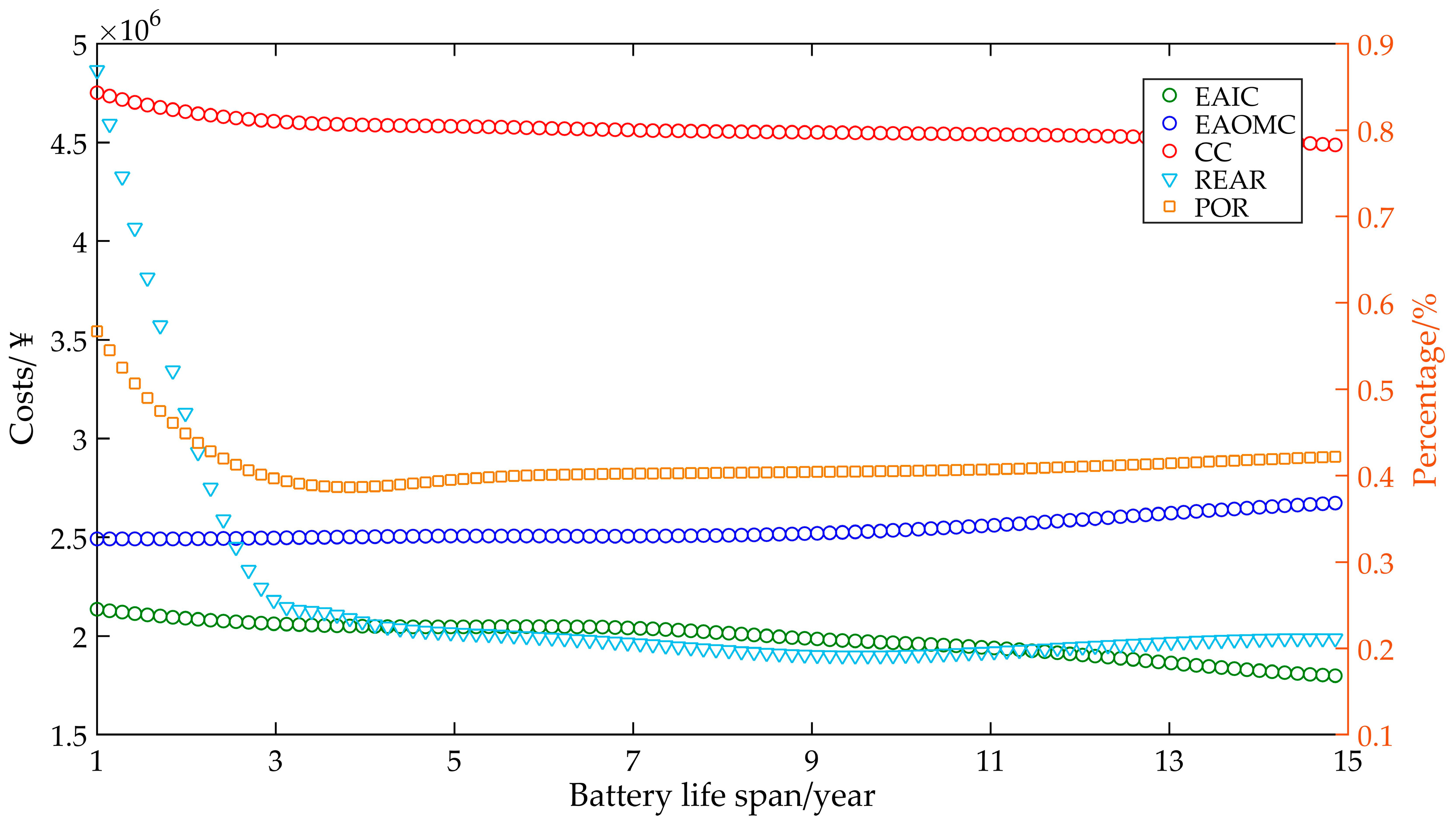
6.6.1. Influence of Battery Life Span on Planning Results

The battery life span is directly related to the EAIC of the system, and thus affects the CC of the whole system and other indicators. With the improvement of battery technology, the impact of the change in the battery life span on the system planning results must be considered. As the battery life span varies from 1 to 15 (in steps of two), the changes in various costs of the HSCES, the renewable energy abandonment rate (REAR) of the SCES and the power outage rate (POR) of the HS, are shown in Figure 13.
As can be seen from Figure 13, when the battery life span becomes longer, the CC of the system gradually decreases. In the range of 1–3 years, the EAIC of the system will be reduced, the REAR and POR of the system will be significantly reduced, and the system will gradually change from hydrogen storage to hybrid energy storage. In the range of 3–9 years, the system maintains the hybrid energy storage mode, and the EAOMC and POR of the system are basically unchanged. Due to the reduction of the EAIC of the battery, the EAIC of the system is gradually reduced. At the same time, the planned number of batteries will be appropriately increased and the installed capacity of the renewable energy will be reduced. Therefore, the absorption capacity of renewable energy will be improved, while the REAR will be reduced. In the range of 9–15 years, the system will gradually be changed from hybrid energy storage to battery energy storage. The system’s REAR and POR remained at a low ratio. At the same time, the system’s EAIC and CC continued to decrease and reached the lowest value in the range.

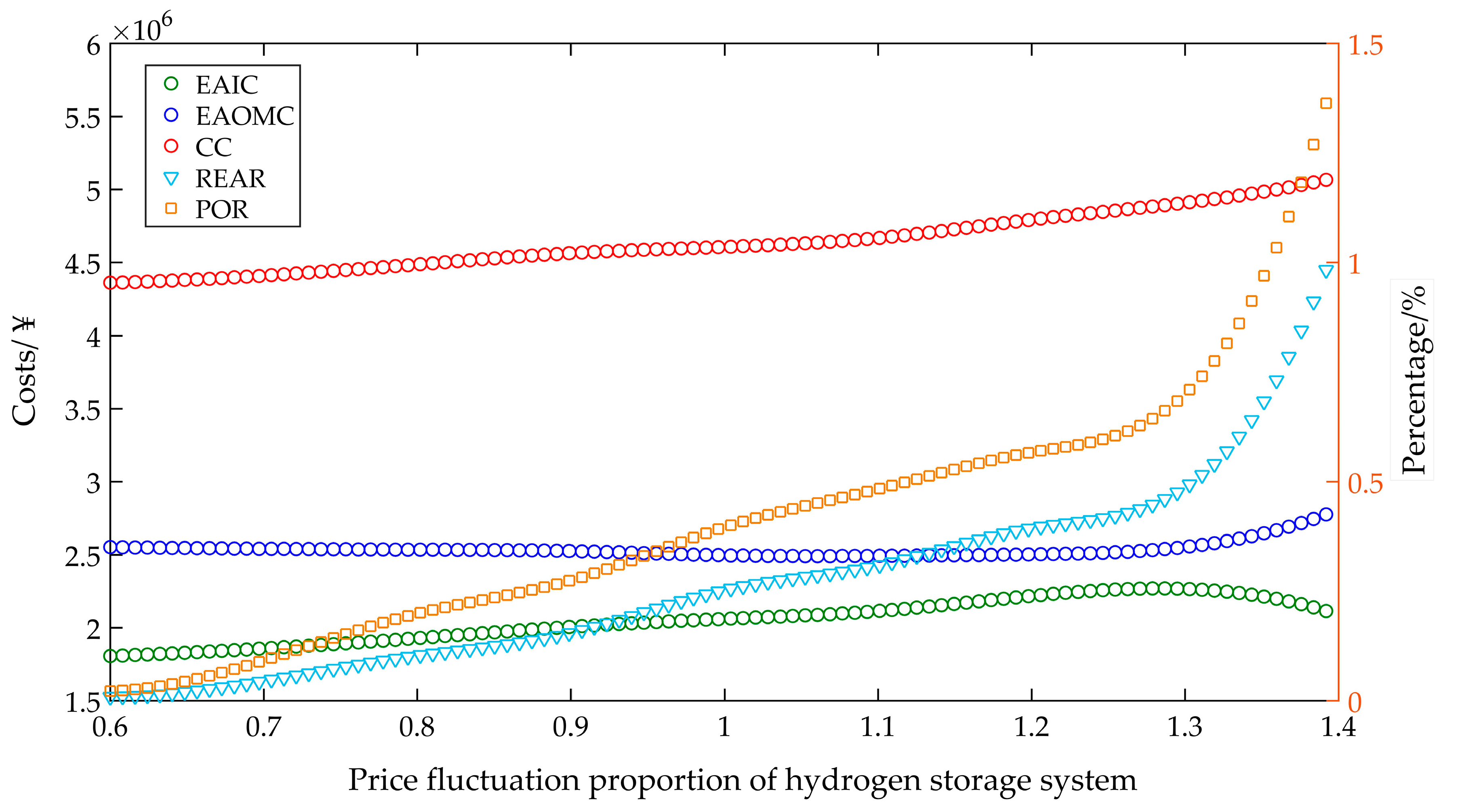
6.6.2. Influence of Hydrogen Storage System Price on Planning Results

The price fluctuation of the hydrogen storage system is related to the changes of various cost coefficients, the renewable energy utilization rate and the power supply reliability of the system. Therefore, it is essential to research how pricing changes affect hydrogen storage systems in the planning results of the HSCES. When the price ratio of the hydrogen storage system changes between 0.6 and 1.4 when compared to the current price (in steps of 0.1), the changes in various costs of the HSCES, the REAR of the SCES and the POR of the HS are shown in Figure 14.
Figure 14 demonstrates that as the price of the hydrogen storage system rises, the EAICs of the system increases significantly in the price ratio range from 0.6 to 1.3, as well as shows a rapid downward trend. It indicates that the system adopts the hybrid energy storage method when the price ratio of the hydrogen storage system fluctuates between 0.6 and 1.3. When the price of the hydrogen storage system increases, the initial capital cost of the system increases. When the price of the hydrogen storage system reaches a certain level, the proportion of the hydrogen storage system within the hybrid energy storage system will be drastically reduced to cut down the system’s overall cost. Therefore, the EAICs of the system will drop sharply. The system EAOMCs remain unchanged in the range between 0.6 and 1.3 of the price ratio fluctuation in the hydrogen storage system, and then shows a rapid upward trend. This is because when the price fluctuation range of hydrogen storage systems is between 0.6 and 1.3, the proportion of battery and hydrogen storage systems in the hybrid energy storage system basically remains unchanged. When the price of hydrogen storage systems reaches a certain level, the proportion of batteries in the hybrid energy storage system and the number ofcharging and discharging batteries will increase. Therefore, system operation and maintenance costs will rise accordingly. With the change of the hydrogen storage system within the price ratio range from 0.6 to 1.4, the REAR and the POR of the system rise slowly at first, and show an explosive growth trend after 1.3 times the node, because at this time, the system is converted from hybrid energy storage to battery energy storage.
To sum up, combined system costs, the REAR and the POR, all maintain a positive correlation with the price of the hydrogen storage system. In the future, with the improvement of battery performance and a reduction in the hydrogen storage system price, the indicators of the system will also perform better. Therefore, the HSCES planning method proposed in this paper has considerable engineering application value, and will be more adaptive and popular in the future.

7. Conclusions

In order to adapt to the gradual integration development of the ES and the HS, this paper proposes a HSCES planning method, which incorporates uncertain wind and PV output and coordinates the configuration of a distributed energy system and an energy storage system. According to the real data from the highway in Western China, we carried out the simulation verification and obtained the following conclusions:
(1)
Under the optimal planning scheme, the HSCES can realize continuous and stable operation. The renewable energy utilization rate of the system is 99.61% and the power supply reliability rate is 99.74%, which reflects the high renewable energy utilization rate and the power supply reliability of the system;
(2)
After introducing the hydrogen storage system, the system can flexibly program the number of micro-generators according to the load demand, significantly reduce the number of distributed energy and battery configurations, and improve the system’s economy;
(3)
Compared with the single power storage system and hydrogen storage system, the combined costs of the hybrid energy storage system are reduced by 2.72% and 6.56%; the renewable energy abandonment rate is reduced by 1.29% and 1.91%; and the power outage rage is reduced by 5.95% and 2.06%, respectively. The hybrid energy storage system is more economical, environmentally friendly and reliable;
(4)
With cost reduction gradually affecting the hydrogen storage system, various indicators within the system will perform better, and the investment potential and engineering application value of the HSCES will be further improved.

Author Contributions

Conceptualization, R.S. and Y.G.; methodology, R.S. and Y.G.; Project administration, R.S.; software, Y.G. and J.N.; validation, R.S., L.J.; Data curation, Y.G., J.N. and K.T.; writing—original draft preparation, Y.G.; writing—review and editing, Y.G., J.N. and K.T.; visualization, Y.G.; supervision, R.S. and L.J. All authors have read and agreed to the published version of the manuscript.

Funding

This research is financially supported by the National Key R&D plan Foundation of China (Grant No. 2021YFB2601300, 2021YFB1600200).

Institutional Review Board Statement

Not applicable.

Informed Consent Statement

Informed consent was obtained from all subjects involved in the study.

Data Availability Statement

The data that support the findings of this study are available from the corresponding author upon reasonable request.

Conflicts of Interest

The authors declare no conflict of interest.

References

  1. Wang, K.; Yu, J.; Yu, Y.; Qian, Y.; Zeng, D.; Guo, S.; Xiang, Y.; Wu, J. A survey on energy internet: Architecture, approach, and emerging technologies. IEEE Syst. J. 2017, 12, 2403–2416. [Google Scholar] [CrossRef]
  2. Sun, H.; Guo, Q.; Wu, W.; Wang, B.; Zhang, B. Integrated energy management system with multi-energy flow for Energy Internet: Design and application. Autom. Electr. Power Syst. 2019, 43, 122–128. [Google Scholar]
  3. Hu, H.; Zhang, Z.; He, Z.; Wang, K.; Yang, X.; Wei, W. The framework and key technologies of traffic energy internet. Proc. CSEE 2018, 38, 12–24. [Google Scholar]
  4. Jia, L.; Shi, R.; Ji, L.; Wu, P. Road Transportation and Energy Integration Strategy in China. Strateg. Study CEA 2022, 24, 163–172. [Google Scholar] [CrossRef]
  5. Sahraei, M.A.; Duman, H.; Çodur, M.Y.; Eyduran, E. Prediction of transportation energy demand: Multivariate adaptive regression splines. Energy 2021, 224, 120090. [Google Scholar] [CrossRef]
  6. Jin, L.; Zhang, B.; Zhang, L.; Yang, W. Nanogenerator as new energy technology for self-powered intelligent transportation system. Nano Energy 2019, 66, 104086. [Google Scholar] [CrossRef]
  7. Jia, L.; Shi, R.; Ma, J. Research on the Energy Potential of Land Transportation Infrastructure Assets in China; Science Press: Beijing, China, 2020. [Google Scholar]
  8. Jia, L.; Shi, R.; Ji, L. Research Report on Integrated Development Strategy of Rail and Road Transportation and Energy—Road; Strategic Consulting Report of Chinese Academy of Engineering: Beijing, China, 2022. [Google Scholar]
  9. Ji, L.; Yu, Z.; Ma, J.; Jia, L.; Ning, F. The potential of photovoltaics to power the railway system in China. Energies 2020, 13, 3844. [Google Scholar] [CrossRef]
  10. Hagos, D.A.; Ahlgren, E.O. Exploring cost-effective transitions to fossil independent transportation in the future energy system of Denmark. Appl. Energy 2020, 261, 114389. [Google Scholar] [CrossRef]
  11. Salvi, B.L.; Subramanian, K.A. Sustainable development of road transportation sector using hydrogen energy system. Renew. Sustain. Energy Rev. 2015, 51, 1132–1155. [Google Scholar] [CrossRef]
  12. Jia, L.; Ma, J.; Cheng, P.; Liu, Y. A perspective on solar energy-powered road and rail transportation in China. CSEE J. Power Energy Syst. 2020, 6, 760–771. [Google Scholar]
  13. Liu, Z.; Fei, T. Road PV production estimation at city scale: A predictive model towards feasible assessing regional energy generation from solar roads. J. Clean. Prod. 2021, 321, 129010. [Google Scholar] [CrossRef]
  14. Kim, H.G.; Hwang, H.J.; Kang, Y.H.; Yun, C.Y. Evaluation of onshore wind resource potential according to the road proximity. New Renew. Energy 2013, 9, 13–18. [Google Scholar] [CrossRef]
  15. Zhang, L.; Liu, L.; Wang, M.; Wang, Y.; Zhou, Y. Forecast and analysis of road transportation energy demand under the background of system dynamics. IOP Conf. Ser. Earth Environ. Sci. 2019, 252, 052043. [Google Scholar] [CrossRef]
  16. García-Olivares, A.; Solé, J.; Osychenko, O. Transportation in a 100% renewable energy system. Energy Convers. Manag. 2018, 158, 266–285. [Google Scholar] [CrossRef]
  17. Burandt, T.; Xiong, B.; Löffler, K.; Oei, P.Y. Decarbonizing China’s energy system–Modeling the transformation of the electricity, transportation, heat, and industrial sectors. Appl. Energy 2019, 255, 113820. [Google Scholar] [CrossRef]
  18. Lund, H.; Mathiesen, B.V. Energy system analysis of 100% renewable energy systems—The case of Denmark in years 2030 and 2050. Energy 2009, 34, 524–531. [Google Scholar] [CrossRef]
  19. Ning, F.; Ji, L.; Ma, J.; Jia, L.; Yu, Z. Research and analysis of a flexible integrated development model of railway system and photovoltaic in China. Renew. Energy 2021, 175, 853–867. [Google Scholar] [CrossRef]
  20. Zhang, D.; Kang, Y.; Ji, L.; Shi, R.; Jia, L. Coevolution and Evaluation of Electric Vehicles and Power Grids Based on Complex Networks. Sustainability 2022, 14, 7052. [Google Scholar] [CrossRef]
  21. He, D.; Wang, X.; Zhang, F. Research of Traffic Energy System and Optimization Operation Unified Model. In Proceedings of the 2019 IEEE 3rd International Electrical and Energy Conference (CIEEC), Beijing, China, 7–9 September 2019; pp. 1809–1814. [Google Scholar]
  22. Yan, M.; Li, G.; Li, M.; He, H.; Xu, H.; Liu, H. Hierarchical predictive energy management of fuel cell buses with launch control integrating traffic information. Energy Convers. Manag. 2022, 256, 115397. [Google Scholar] [CrossRef]
  23. Wang, C.; Wang, S.; Gao, Z.; Song, Z. Effect evaluation of road piezoelectric micro-energy collection-storage system based on laboratory and on-site tests. Appl. Energy 2021, 287, 116581. [Google Scholar] [CrossRef]
  24. Wu, T.; Liu, S.; Ni, M.; Zhao, Y.; Shen, P.; Rafique, S.F. Model design and structure research for integration system of energy, information and transportation networks based on ANP-fuzzy comprehensive evaluation. Glob. Energy Interconnect. 2021, 1, 137–144. [Google Scholar]
  25. Farahani, S.S.; Veen, R.; Oldenbroek, V.; Alavi, F.; Lee, E.H.P.; Wouw, N.; Lukszo, Z. A hydrogen-based integrated energy and transport system: The design and analysis of the car as power plant concept. IEEE Syst. Man Cybern. Mag. 2019, 5, 37–50. [Google Scholar] [CrossRef]
  26. Yang, T.; Guo, Q.; Sheng, Y.; Sun, H. Coordination of urban integrated electric power and traffic network from perspective of system inter connection. Autom. Electr. Power Syst. 2020, 44, 1–9. [Google Scholar]
  27. He, Z.; Xiang, Y.; Liao, K.; Yang, J. Demand, Form and Key Technologies of Integrated Development of Energy-Transport-Information Networks. Autom. Electr. Power Syst. 2021, 45, 73–86. [Google Scholar]
  28. Huang, Y.; Guo, H.; Liao, C.; Zhao, D. Research on the Transport Energy Transformation Route of the Guangdong-Hong Kong-Macao Greater Bay Area Based on the Long-range Energy Alternatives Planning System Model. Sci. Technol. Manag. Res. 2021, 41, 209–218. [Google Scholar]
  29. Wei, W.; Danman, W.U.; Qiuwei, W.U.; Shafie-Khah, M.; Catalao, J. Interdependence between transportation system and power distribution system: A comprehensive review on models and applications. J. Mod. Power Syst. Clean Energy 2019, 7, 433–448. [Google Scholar] [CrossRef]
  30. Hamad, A.A.; Nassar, M.E.; EI-Saadany, E.F.; Salama, M.M.A. Optimal configuration of isolated hybrid AC/DC microgrids. IEEE Trans. Smart Grid 2018, 10, 2789–2798. [Google Scholar] [CrossRef]
  31. Pradhan, A.; Panda, B.; Mannepalli, R. Case Studies on Microgrid Design Using Renewable Energy Sources. In Microgrids, 1st ed.; Narejo, G.B., Acharya, B., Singh, R.S.S., Newagy, F., Eds.; CRC Press: Boca Raton, FL, USA, 2021; pp. 279–299. [Google Scholar]
  32. Doost, M.F.; Keshtkar, H.; Gendell, B. Intelligent Roadways: Learning-Based Battery Controller Design for Smart Traffic Microgrid; Springer: Berlin/Heidelberg, Germany, 2020; pp. 998–1011. [Google Scholar]
  33. Liu, Y.; Wang, Y.; Li, Y.; Gooi, H.B.; Xin, H. Multi-agent based optimal scheduling and trading for multi-microgrids integrated with urban transportation networks. IEEE Trans. Power Syst. 2020, 36, 2197–2210. [Google Scholar] [CrossRef]
  34. Chandak, S.; Rout, P.K. The implementation framework of a microgrid: A review. Int. J. Energy Res. 2021, 45, 3523–3547. [Google Scholar] [CrossRef]
  35. Azaza, M.; Wallin, F. Multi objective particle swarm optimization of hybrid micro-grid system: A case study in Sweden. Energy 2017, 123, 108–118. [Google Scholar] [CrossRef]
  36. Zhang, D.; Miao, S.; Zhao, J.; Tu, Q.; Liu, H. A Bi-Level Locating and Sizing Optimal Model for Poverty Alleviation PVs Considering the Marketization Environment of Distributed Generation. Trans. China Electrotech. Soc. 2019, 34, 1999–2010. [Google Scholar]
  37. Guan, L.; Zhao, Q.; Zhou, B.; Lyu, Y.; Zhao, W.; Yao, W. Multi-scale clustering analysis based modeling of photovoltaic power characteristics and its application in prediction. Autom. Electr. Power Syst. 2018, 42, 24–30. [Google Scholar]
  38. Yuan, G.; Gao, Y.; Ye, B. Optimal dispatching strategy and real-time pricing for multi-regional integrated energy systems based on demand response. Renew. Energy 2021, 179, 1424–1446. [Google Scholar] [CrossRef]
  39. Zhang, C.; Cai, J.; Zhang, Y.; Du, S.; Sun, Z.; Xu, D. Simulation of high temperature solid oxide water electrolysis for hydrogen production based on thermodynamic equilibrium. Acta Energ. Sol. Sin. 2021, 42, 210–217. [Google Scholar]
  40. Ni, M.; Leung, M.K.; Leung, D.Y. Energy and exergy analysis of hydrogen production by a proton exchange membrane (PEM) electrolyzer plant. Energy Convers. Manag. 2008, 49, 2748–2756. [Google Scholar] [CrossRef]
  41. Xu, Y.; Dong, Z.; Zhang, R.; Hill, D. Multi-timescale coordinated volt-age/var control of high renewable-penetrated distribution systems. IEEE Trans. Power Syst. 2017, 32, 4398–4408. [Google Scholar] [CrossRef]
  42. Wais, P. Two and three-parameter Weibull distribution in available wind power analysis. Renew. Energy 2017, 103, 15–29. [Google Scholar] [CrossRef]
  43. Yu, J.; Fu, Y.; Yu, Y.; Wu, Y.; Wu, S.; Song, L. Research on two-parameters wind resource assessment methods in BOHAI sea. Acta Energ. Sol. Sin. 2021, 42, 325–332. [Google Scholar]
  44. Cai, J.; Hao, L.; Xu, Q.; Zhang, K. Reliability assessment of renewable energy integrated power systems with an extendable Latin hypercube importance sampling method. Sustain. Energy Technol. Assess. 2022, 50, 101792. [Google Scholar] [CrossRef]
  45. Mohseni, S.; Brent, A.C.; Burmester, D.A. Comparison of metaheuristics for the optimal capacity planning of an isolated, battery-less, hydrogen-based micro-grid. Appl. Energy 2020, 259, 114224. [Google Scholar] [CrossRef]
  46. Sufyan, M.; Rahim, N.A.; Aman, M.M.; Tan, C.K.; Raihan, S.R.S. Sizing and applications of battery energy storage technologies in smart grid system: A review. J. Renew. Sustain. Energy 2019, 11, 014105. [Google Scholar] [CrossRef]
  47. Khalid, A.; Stevenson, A.; Sarwat, A.I. Overview of technical specifications for grid-connected microgrid battery energy storage systems. IEEE Access. 2021, 9, 163554–163593. [Google Scholar] [CrossRef]
Figure 1. A scenario with the HSCES.
Sustainability 15 03166 g001
Figure 2. The architecture of the HSCES.
Sustainability 15 03166 g002
Figure 3. Operation control strategy flow of the HSCES.
Sustainability 15 03166 g003
Figure 4. Function–carrier–energy consumption diagram of the HS.
Sustainability 15 03166 g004
Figure 5. The HSCES wiring topology diagram.
Sustainability 15 03166 g005
Figure 6. Flow chart of micro-generator planning for the HSCES.
Sustainability 15 03166 g006
Figure 7. (a) Weather information in spring; (b) weather information in summer; (c) weather information in autumn; (d) weather information in winter.
Sustainability 15 03166 g007
Figure 8. Annual load data of the HSCES.
Sustainability 15 03166 g008
Figure 9. Set of wind and PV scenarios.
Sustainability 15 03166 g009
Figure 10. Typical scenarios for wind output.
Sustainability 15 03166 g010
Figure 11. Typical scenarios for PV output.
Sustainability 15 03166 g011
Figure 12. (a) Output of renewable energy; (b) output of the hybrid energy storage system; (c) remaining capacity ratio of the hybrid energy storage system; (d) overall operation of the HSCES.
Sustainability 15 03166 g012
Figure 13. Influence of the battery life span on the planning results.
Sustainability 15 03166 g013
Figure 14. Influence of price fluctuation of the hydrogen storage system on the system.
Sustainability 15 03166 g014
Table 1. Full text nomenclature description table.
Nomenclature n t Number of Toll Stations
P L o a d Load power, kW L r The total length of the highway, km
P r e s Renewable energy output, kW P i , m , t F C Power prediction value of typical seasonal scenario m at the time t , kW
E b a t Remaining capacity of the battery, kWh P i , t F C Power value at the time t obtained from historical power prediction, kW
m i n E b a t Lower limit of battery capacity, kWh ξ i Wide range of prediction error
m a x E b a t Upper limit of battery capacity, kWh R i , t Obey some random distribution
P c b a t Battery charging power, kW λ Random distribution correction factor
m a x P c b a t Maximum charging power of the battery, kW c Shape parameters of Weibull distribution
P d b a t Battery discharging power, kW k Scale parameters of Weibull distribution
m a x P d b a t Maximum discharging power of the battery, kW v ¯ Average wind speed, m/s
H b a t Remaining capacity of hydrogen storage tank, kg σ Standard deviation
m i n H b a t Lower limit of hydrogen storage tank capacity, kg Γ ( 1 + 1 / k ) Gamma function
m a x H b a t Upper limit of hydrogen storage tank capacity, kg α Shape parameters of beta distribution
P f c Hydrogen fuel cell output, kW β Scale parameters of beta distribution
m a x P f c Maximum output of hydrogen fuel cell, kW N d Normalization factor
P e l e Electrolysis cell power output, kW D i Scenario probability distance
m a x P e l e Maximum output power of electrolysis cell, kW λ i Scenario probability
c v Calorific value of hydrogen, kWh/kg d ( x a , x b ) Euclidean distance
S e l e Hydrogen production efficiency of the electrolysis cell n s o Number of initial scenarios
S f c Conversion efficiency of hydrogen fuel cell D min Nearest probability distance
P w Wind power output, kW C i n i t i a l Initial capital cost, ¥
S Actual wind speed, m/s C o m Operation and maintenance cost, ¥
S c i Cut-in wind speed, m/s n k Service life of each micro-generator, year
S c o Cut-out wind speed, m/s N m Installation number of each micro-generator
S r a Rated wind speed of wind turbine, m/s P m Rated output power of each micro-generator, kW
P r a Rated power of wind turbine, kW U m Investment cost of unit power of each micro-generator, ¥
P s Rated power of PV panel, kW L m Service life of each micro-generator, year
G ( φ , m , d , h ) Solar radiation intensity at latitude φ , in the m month, d day, h hour, W/m2 r Fund discount rate
θ T Temperature coefficient of PV panel, °C M m Unit power operation and maintenance cost, ¥
T Actual temperature of PV panel, °C Q ( t ) t , kWh
T r e f Reference temperature of PV panel, °C Q l ( t ) Insufficient power at the time t , kWh
β Battery self-discharge rate U r e n Renewable energy utilization rate
η c b a t Battery charging efficiency E r e n Renewable energy power generation, kW
η d b a t Battery discharging efficiency E e x c e s s Renewable energy abandonment power, kW
C b a t Rated capacity of the battery, kWh p w t t , kW
η ele Electrolysis cell efficiency p p v t , kW
P ele i n Input power of electrolytic cell, kW S O C min Lower limit of battery state of charge
E Q h 2 ( t ) The hydrogen storage tank stores energy at the time t , kW S O C max Upper limit of battery state of charge
η f c Hydrogen fuel cell efficiency P max d 1 Maximum discharge power of a battery, kW
P f c i n Input power of hydrogen fuel cell, kW P max c 1 Maximum charging power of a battery, kW
Q c , c { F , S , Q , T , R } Energy consumption of highway system infrastructure, kW P max e l e 1 Maximum output of one electrolysis cell, kW
q i 1 ( t ) Energy   consumption   of   the   i t h service area for one hour, kWh P max f c 1 Maximum output of one hydrogen fuel cell, kW
q j 2 ( t ) Energy consumption of the j t h parking area for one hour, kWh S O C m i n H 2 Lower limit of hydrogen storage tank capacity status
L S Tunnel length, m S O C m a x H 2 Upper limit of hydrogen storage tank capacity status
n S Number of tunnels Q m a x H 2 Maximum capacity of one hydrogen storage tank, kg
L B Bridge length, km
This table is a continuation of the one above.
Table 2. Hydrogen-fueled internal combustion engine and hydrogen fuel cell comparison.
TypeHydrogen Fuel CellHydrogen-Fueled Internal Combustion Engine
Emissions2H2 + O2 = 2H2O2H2 + O2 = 2H2O
2H2→4H+ + 4e + O2→2H2OH2 + O2 + N2→H2O + NOX
Efficiency50~60%, theoretical up to 90%25~30%
Reservoir densityHighLow
Storage tankSmallLarge
Table 3. Related parameters of the different equipment.
EquipmentSpecification ParametersICC
(¥/kW)
OMC
(¥/kW)
Life Span
(Year)
Wind turbines100 kW85000.01820 year
PV panels2 kW11,0000.00720 year
Batteries12 V/100 A·h10000.083 year
Electrolysis cell1 kW13000.0310 year
Hydrogen storage tanks1 kg180020 year
Hydrogen fuel cells1 kW11000.0410 year
Table 4. Typical scenario probabilities of wind and PV.
TypeScenario 1Scenario 2Scenario 3Scenario 4Scenario 5
wind0.1450.1150.1150.1900.435
PV0.0800.1100.3350.3350.120
Table 5. Combined scenario probabilities.
Scenario12345678910111213
Probability0.0120.0170.0490.0490.0180.0100.0130.0400.0400.0140.0100.0130.040
Scenario141516171819202122232425
Probability0.0400.0140.0160.0210.0640.0640.0240.0360.0490.1470.1470.053
Table 6. Simulation results of three experimental design schemes.
Experiment Design SchemeOptimal ValueAverage ValueVariance
Scheme 1 473.14473.531.3
Scheme 2 492.35492.971.7
Scheme 3 459.58460.652.6
Table 7. Results of micro-generator planning.
Experiment DesignWind TurbinesPV PanelsBatteriesElectrolysis CellsHydrogen Storage TanksHydrogen Fuel Cells
Scheme 1 19573485000
Scheme 2 1954507749183
Scheme 3 18550264512378
Table 8. Results of each index.
Experiment DesignEAIC/¥EAOMC/¥EAC/¥REAR/¥POR/¥Combined Costs (CC)/¥
Scheme 1 1,726,0502,416,0404,142,0901.68%6.21%4,735,370
Scheme 2 2,382,0402,200,4004,582,4402.30%2.32%4,929,668
Scheme 3 2,061,1302,496,4004,557,5300.39%0.26%4,606,472
Disclaimer/Publisher’s Note: The statements, opinions and data contained in all publications are solely those of the individual author(s) and contributor(s) and not of MDPI and/or the editor(s). MDPI and/or the editor(s) disclaim responsibility for any injury to people or property resulting from any ideas, methods, instructions or products referred to in the content.

