Image Segmentation of Cucumber Seedlings Based on Genetic Algorithm

Abstract

To solve the problems of the low target-positioning accuracy and weak algorithm robustness of target-dosing robots in greenhouse environments, an image segmentation method for cucumber seedlings based on a genetic algorithm was proposed. Firstly, images of cucumber seedlings in the greenhouse were collected under different light conditions, and grayscale histograms were used to evaluate the quality of target and background sample images. Secondly, the genetic algorithm was used to determine the optimal coefficient of the graying operator to further expand the difference between the grayscale of the target and background in the grayscale images. Then, the Otsu algorithm was used to perform the fast threshold segmentation of grayscale images to obtain a binary image after coarse segmentation. Finally, morphological processing and noise reduction methods based on area threshold were used to remove the holes and noise from the image, and a binary image with good segmentation was obtained. The proposed method was used to segment 60 sample images, and the experimental results show that under different lighting conditions, the average F1 score of the obtained binary images was over 94.4%, while the average false positive rate remained at about 1.1%, and the image segmentation showed strong robustness. This method can provide new approaches for the accurate identification and positioning of targets as performed by target-dosing robots in a greenhouse environment.

1. Introduction

Plant segmentation, which involves classifying image pixels into foreground (crops and weeds) and background (soil) according to the job requirements, is one of the key technologies in precision agriculture, such as in weed identification and crop disease detection [1,2,3]. In terms of the target recognition of an automatic target-spraying robot, the lighting conditions, the shadows of the plant, the color and morphology of the plant, and the presence of a complex background can all affect plant segmentation, so establishing a more robust image segmentation method is a current research hotspot [4,5,6].

With a green plant as the target, the most commonly used image segmentation methods are based on the color index or learning. The former improves the segmentation effect based on the color index. For example, Woebbecke et al. [7] proposed the Excess Green Index (ExG), which emphasizes plant greenness and can effectively separate the plant from the soil. In order to simulate human color perception, Meyer et al. [8] proposed the Excess Red Index (ExR), considering the relative ratios of the three types of cones in the human eye. This approach can also effectively separate plants and soil but is not as accurate as ExG. In addition, there are also CIVE, ExGR, and other color indices [9,10]. Guijarro et al. [11] combined four green indices (ExG, CIVE, ExGR, and VEG) to improve segmentation quality and created a combinatorial index called COM1. This method has been tested in barley and corn fields and has shown strong reliability. Researchers are also constantly exploiting new color indices to improve the quality of plant segmentation [6]. It can be seen that segmentation methods based on the color index achieve good segmentation results in specific scenes, but these methods still face certain limitations in the face of complex environments and changing illumination.

In addition to the image segmentation method based on the color index, Yang et al. [12] proposed an HSV- and color deviation-based method for greenness identification, which achieved good results under different environmental conditions, and its percentage of error averaged 8.31%. However, when the light was too dark or too bright, the method achieved poor results. In the study of tomato leaf segmentation, Tian et al. [13] used a K-means algorithm based on the adaptive cluster number, which can successfully segment tomato leaf images more precisely and efficiently than the traditional K-means algorithm (an unsupervised prototype clustering method that classifies objects by computing the distance from the cluster center), DBSCAN algorithm (a clustering method based on density), mean shift algorithm (a clustering method based on mean shift), and ExG-ExR color indices method (a threshold segmentation method), while its running time was slightly slower than that of the ExG-ExR method. Deep learning methods, such as convolutional neural networks (CNN), are widely used in crop identification [14,15]. Ngugi et al. [16] proposed a tomato leaf segmentation algorithm based on deep learning, and the proposed segmentation network KijaniNet outperformed all competitors, with a boundary F1 score of 0.9439. In addition, all CNN models performed the segmentation of a 256 × 256-pixel RGB image in under 0.12 s when running on a GPU. Although these kinds of image segmentation methods based on learning can achieve good recognition, they rely on a large number of data sets to train the model. Moreover, these methods have increased computation times, which is not preferable for use in real-time applications.

Due to the greenness properties of green plants, most researchers conduct plant identification studies based on RGB images. While multispectral and hyperspectral cameras can obtain more spectral information, they suffer from data redundancy and high costs. The greenhouse is the main environment of vegetable and fruit seedlings, and the complex background environment (nutrient soil and seedling trays), lighting conditions, shadows of plants, and other factors here affect the image segmentation of plant seedlings. Accurate plant identification is fundamental to the robot-based spraying mission, which typically consists of image acquisition, target identification, localization, and treatment distribution. In this study, an image segmentation method based on the genetic algorithm (GA) is proposed to identify cucumber seedlings accurately and quickly so as to successfully perform accurate and rapid target-spraying tasks.

2. Image Acquisition and Method Flow

2.1. Image Acquisition Method

In agricultural production, when the cucumber seedling has one or two true leaves, ethephon is sprayed on the leaves multiple times to accelerate female flower differentiation. In this study, cucumber seedlings are taken as the target object. The plants were grown in a seedling tray inside the glasshouse of the Guantang Experimental Farm of Zhejiang A&F University. About 30 seedlings were scanned when the second true leaf appeared using the OV560 camera module from SingTown, and the shooting was carried out in early May 2022. The camera’s lens focal length is 2.8 mm, its horizontal field of view angle is 70.8°, and its vertical field of view angle is 55.6°. In order to meet the spraying requirements under realistic conditions and to make the seedlings appear in the appropriate position in the image, the lens was fixed about 55 cm away from the seedling tray, and the camera shot vertically towards the ground, as shown in Figure 1.

A total of 60 images were collected as tests to verify the performance of the method, including 20 images collected in bright light (11 a.m.–1 p.m., in sunny weather), 20 images collected in weak light (around 5 p.m.), and 20 images collected in normal light (sunny morning, or cloudy weather). In addition, nine were selected as sample images (including three images with strong light, three with weak light, and three with normal light conditions) to obtain sample pixels (the plant and the background) and area thresholds (in the noise reduction process). The format of the collected images was generalized as .jpg. The resolution of each image was 1200 × 1200 pixels.

2.2. Image Processing Workflow

The GA-based segmentation method for cucumber seedlings is mainly divided into five steps, as shown in Figure 2. Firstly, two kinds of sample pixels from the plant and the background were collected, and the evaluation metrics of grayscale histograms were designed. Two kinds of sample pixels and evaluation metrics were substituted into the GA process to obtain the optimal coefficients of the grayscale operator. Secondly, a fresh grayscale operator was used to grayscale the input color image. Then, the coarse segmentation of the binary image was performed by thresholding the image using the Otsu algorithm. Morphology was then used to smooth the boundaries and remove white holes and some noise. Finally, a threshold-based noise reduction method was used to remove large areas of noise from the image.

3. Grayscale Process

Image grayscale is an image preprocessing method. On the one hand, color images can be transformed from three channels (such as the R, G, and B channels of RGB images) into one via certain grayscale methods, which simplifies the image matrix and improves the computing speed. On the other hand, the contributions of different channels are highlighted by a reasonable setting of the coefficient weights, leading to better segmentation results. When segmenting a green plant, a fixed grayscale operator is typically adopted based on the color characteristics. Currently, the most commonly used grayscale operators include ExG (2G-R-B), G-B, G-R, CIVE (−0.811G + 0.441B + 0.385R), and EXG-EXR (3G-2.4R-B) of RGB color space (Hamuda et al., 2016). The value of each component in the RGB color model is related to the brightness of the pixels; thus, factors such as illumination, soil, weeds, seedling disks, shadows, and dead leaves can affect the grayscale process and segmentation effect of the image.

As a result, the optimal grayscale operator will vary depending on the actual environment. The mathematical expression of Gray, the grayscale operator of the RGB model, is as follows:

$$Gary=a\times \mathrm{G}+b\times \mathrm{B}+c\times \mathrm{R}+d$$

(1)

where Gray represents the calculated gray value, with a value range of [0, 255]; G, B, and R represent the pixel values of the green, blue, and red channels in the color image, respectively; and a, b, and c represent the calculated weights of the color channels G, B, and R in the color image, respectively. The term d is the correction constant.

3.1. Preparation of GA

3.1.1. Sample Image Selection

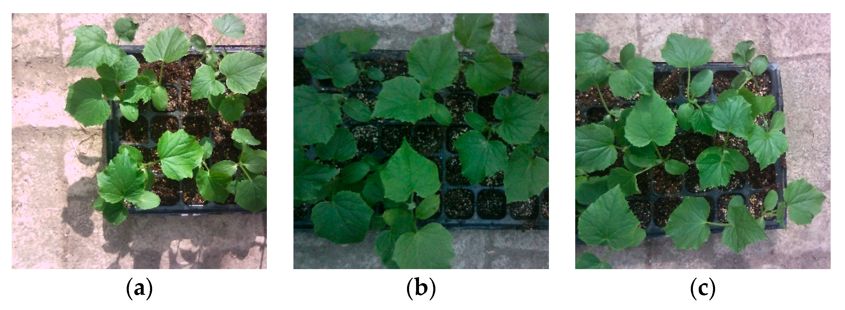
Sample images under three lighting conditions were selected from the collected images, as shown in Figure 3. It can be seen that the collected images contain cucumber seedlings, nutrient soil, seedling trays, and additional information. Cucumber seedlings are classified as plant, and the green features are clear, while other features are classified as non-plant and have no obvious color features.

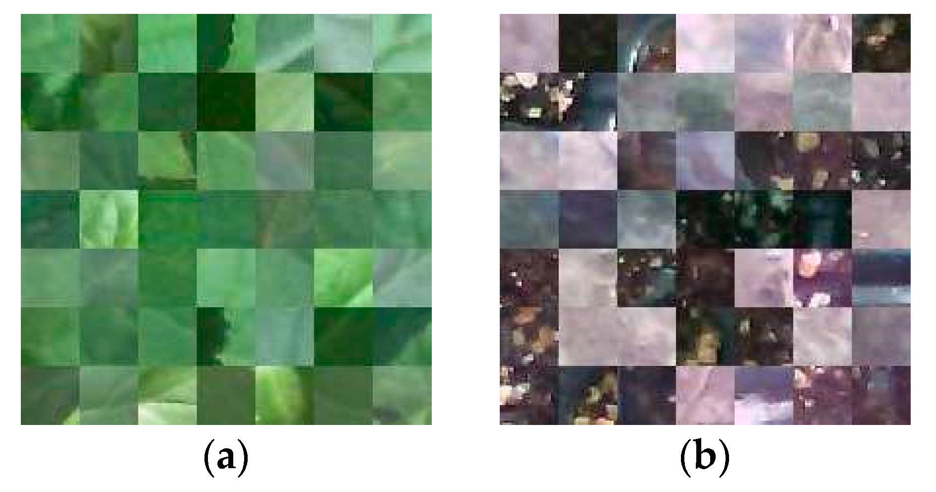
In order to reduce the presence of unnecessary data, improve the computing speed of the genetic algorithm, and facilitate the comparison and analysis of the gray histogram of the plant and background, Photoshop software was used to manually define 49 plant squares and 49 background squares in the sample images, and the resolution of each square was 30 × 30 pixels. Moreover, they were concatenated into images of plant samples and images of background samples, respectively, to provide pixel information for the GA, as shown in Figure 4.

3.1.2. Evaluation Metrics for the Gray Histogram

In order to achieve a perfect segmentation effect, the ideal grayscale operator should produce large differences between the plant and background. Combining the distribution characteristics of each channel component of the green plant image in RGB color space, the three components of R, G, and B in color space are reassigned for computation, resulting in a grayscale image with higher contrast.

The overlap ratio C_d of plant and background, the mean difference A_d, and the standard deviations σ_q and σ_b of plant and background were set as the evaluation metrics of image segmentation.

The smaller the overlap ratio, the more favorable it is to distinguish the plant from the background after using grayscale. The formula for the overlap ratio C_d is as follows:

$$C_d=\frac{{2N}_d}{N_c}\times 100\%$$

(2)

where N_d is the number of pixels in the coincidence region, and N_c is the total number of pixels of the plant and background.

The larger the mean difference, the more scattered the gray values of the plant and background are in the histogram, which is more favorable for differentiation. The formula for the mean difference A_d is as follows:

$$A_d=\left|m_q-m_b\right|=\left|{\displaystyle \sum }_{k=0}^{255}{kf}_q\left(k\right)-{\displaystyle \sum }_{k=0}^{255}{kf}_b\left(k\right)\right|$$

(3)

where m_q and m_b denote the average grayscale values of the plant and background, respectively; f_q(k) and f_b(k) denote the probabilities of the gray values of plant and background being k, respectively; and k denote the gray value.

The smaller the standard deviation of the plant and background, the smaller the dispersion of the grayscale values of the plant and background pixels, which facilitates the differentiation of plant from background and indirectly improves the stability of the segmentation algorithm. The standard deviations of plant and background σ_q and σ_b can be calculated as follows:

$${\sigma }_q=\sqrt{{\displaystyle \sum }_{k=0}^{255}{\left(k-m_q\right)}^2\times f_q\left(k\right)}$$

(4)

$${\sigma }_b=\sqrt{{\displaystyle \sum }_{k=0}^{255}{\left(k-m_b\right)}^2\times f_b\left(k\right)}$$

(5)

According to the actual effects of performance parameters such as C_d, A_d, σ_q, and σ_b on the distribution of the grayscale values of plant and background, set the positive and negative signs of parameters, and set the weights according to the combination of the bimodal characteristics of the gray histogram and their theoretical value range. The above evaluation metrics are given different weights through calculations and tests, and a correction constant is set to ensure that more fitness is positive (GA will weed out individuals with fitness below zero). Finally, the comprehensive function f(x) used for evaluating the grayscale histogram is constructed as follows:

$$f\left(x\right)=-{35\times C}_d+0{.8\times A}_d-0{.5\times (\sigma }_q{+\sigma }_b)+500$$

(6)

Simultaneously, the comprehensive evaluation function is also used in the fitness function of the subsequent GA.

3.2. GA Flow

GA is a meta-heuristic algorithm based on evolutionary theory, genetics, and the principle of natural selection [17]. By mimicking natural biological evolutionary mechanisms, starting from an initial population of possible solution sets, fresh populations are generated using selection, crossover, and mutation operations, and good individuals are screened with an appropriate fitness function. The population is made to evolve in the optimal direction asymptotically until the optimal solution is found. GA is frequently used in combinatorial optimization and scheduling problems [18,19]. The GA is used to optimize the four coefficients (a, b, c, and d) of the grayscale operator to strengthen the plant and suppress the background. The process is as follows.

3.2.1. Coding Mode and Initial Population

To facilitate gene exchange and mutation, binary coding is used. By referring to operators such as CIVE and 2G−R−B, the value range of the coefficients of these operators is limited to the definition domain of three coefficients (a, b, and c), so that each coefficient has an optimal solution as long as there are enough feasible solutions. Through experiments, the definition domains of the four coefficients are specified, in which a, b, and c ∈ [−10, 10] and d ∈ [−40, 40], and the accuracy of each coefficient is set as 0.01. Then, a, b, and c account for 11 bits, and d accounts for 13 bits. After the combination, the individuals are represented by a 46-bit binary number string code, where the maximum of each number string is the interval length of the domain defined by the corresponding coefficient, and the minimum is zero. During gene expression, the binary is first converted to decimal form, and the final coefficient is obtained by adding the minimum value of the domain of the corresponding coefficient. For example, the code of “1.2R + 2B − B + 21.34” is “10001100000 10010110000 1110000100 1011111110110”. The initial population number is set at 70.

3.2.2. Fitness Function and Genetic Operator

The fitness function is represented by Formula (6). Taking the maximum fitness function as the goal, the grayscale map is obtained by selecting the grayscale operator coefficients of individuals in the population, and then the value calculated by the comprehensive evaluation function (Formula (6)) is used as the corresponding fitness to participate in the calculation.

Genetic operators mainly include selection, crossover, and mutation. The chosen strategy is the roulette selection strategy. The probability formula for individual selection is as follows:

$$P_i=\frac{f_i}{{{\displaystyle \sum }}_{i=1}^n{f}_i}$$

(7)

where P_i is the probability that an individual is selected; f_i is the fitness function of an individual; and n is the total number of individuals in the population.

The crossover probability is set as 0.8 (80%), two chromosomes are randomly selected, and a random number P_c is generated between 0 and 1. If P_c < 0.8, multi-point crossover is used for the crossover operation. The mutation probability is set as 0.09 (9%), a chromosome is randomly selected, and a random number P_m is generated between 0 and 1. If P_m < 0.09, the mutation operation is carried out; that is, the digits are randomly selected on the chromosome for inverting. Moreover, the maximum number of iterations is set to 200.

3.2.3. Calculation Result

Using sample images of plant and background pixels as samples, PyCharm software is used to compute and iterate the above procedure to obtain the iteration curve of the fitness function, which is shown in Figure 5. It can be noted that the evolution is rapid up to 25 generations and the fitness changes tend to flatten out after 25 generations, indicating that the optimal individuals are increasingly difficult to find. Finally, the optimal coefficients a = 4.70, b = −2.00, c = −2.60, and d = −41.36 are obtained; that is, the optimal grayscale operator is Gray = 4.70G − 2.00b − 2.60R − 41.36.

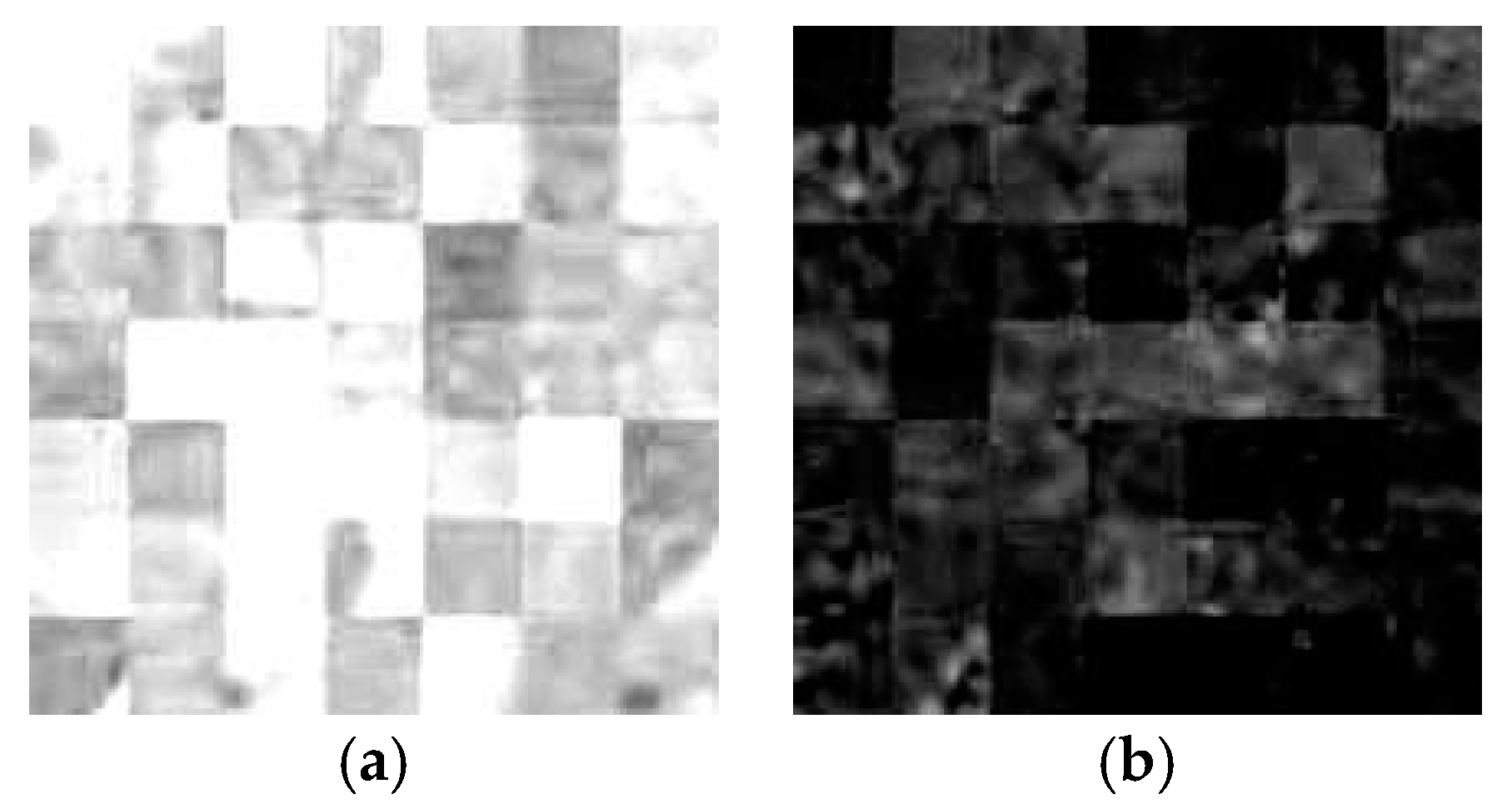
The grayscale histogram distribution of the improved grayscale operator tends to be polarized. In Figure 6b, the grayscale levels 0 and 255 of the grayscale histograms are neglected. It can be seen that the overlap of the grayscale map between the plant and the background is tiny, and the difference is noticeable, showing clear bimodality. The optimized grayscale operator was applied to the grayscale Figure 3d,e, and the resulting grayscale images are shown in Figure 7.

The evaluation metrics C_d, A_d, σ_q, σ_b, and fitness f of each grayscale operator were calculated, and the results are shown in

Table 1. Comparison of evaluation metrics and fitness of each grayscale operator.

Operator	Cd (%)	Ad	σq	σb	f
2G-R-B	0.41	75.69	21.56	5.00	532.58
G-R	3.32	42.58	14.87	4.45	408.20
G-B	1.85	31.81	8.76	3.72	454.52
CIVE	0.49	25.11	0.89	7.33	498.74
3G-2.4B-R	5.81	85.73	38.35	2.73	344.78
Optimal operator	0.45	192.91	33.20	28.65	607.37

.

According to Table 1, the overlap ratio of 2GR-B, CIVE, and the optimal operator is relatively small, while the overlap ratio of the other operators exceeds 1%. The optimal operator has the largest mean difference, while the CIVE operator has the smallest standard deviation of the plant and the 3G-2.4B-R operator has the smallest standard deviation of the background. In general, the optimal operator with the highest fitness f is followed by 2G-R-B, CIVE, and others.

4. Image Segmentation

4.1. Threshold Segmentation Based on Otsu Algorithm

There are numerous methods used to perform threshold segmentation for grayscale images, such as the iterative method, the bimodal method, the Otsu algorithm, and the max-entropy threshold [20]. These methods have their own peculiarities. Considering the histogram features of grayscale images, the processing speed, and the image segmentation effect, the Otsu algorithm [21] can automatically obtain the segmentation threshold with favorable experimental results [22]. The Otsu algorithm used in this paper is based on probabilistic statistics and the least squares principle. By traversing the gray level, the maximum interclass variance is sought to enable automatic threshold selection. If the threshold value t divides the image μ into target μ₁ and background μ₂, then the mathematical expression of the interclass variance σ² is as follows:

$${\sigma }^2{=\omega }_1{\left({\mu }_1-\mu \right)}^2{+\omega }_2{\left({\mu }_2-{\mu }_1\right)}^2$$

(8)

where μ₁ is the average gray value of the target pixel, μ₂ is the average gray value of the background pixel, μ is the average gray value of all pixels in the entire image, ω₁ is the pixel ratio of the target in the entire image, and ω₂ is the pixel ratio of the background in the entire image. The larger the interclass variance, the larger the difference between the target and the background. Therefore, the current t is the optimal threshold when the maximum σ² is found.

Each operator was used to grayscale Figure 3b to obtain the corresponding grayscale image. The binary images were then obtained by performing threshold segmentation using the Otsu algorithm, as shown in Figure 8 and Figure 9.

It can be seen from Figure 8 that the plant part of the grayscale image of the optimal operator is enhanced, while the background part is suppressed. This is in contrast to the grayscale images of G-R, G-B, and CIVE, in which the difference between the plant and the background is not obvious and the boundaries are blurred. The binary images of G-B and 3G-2.4B-R have a large amount of corrupted boundary information, and there is the problem of under-segmentation. The binary image of G-R has numerous voids and much noise. The CIVE binary image shows a certain degree of over-segmentation. 2G-R-B segmented cucumber seedlings effectively but suffered from a small amount of under-segmentation and noise. The optimal operator yielded the most complete segmentation result, but with a certain amount of noise and a few holes.

4.2. Morphological Processing and Noise Reduction

As can be seen in Figure 9, the images after threshold segmentation have black holes and white speckle noise, and particularly show noise caused by yellow-green particles and green weeds in the seedling tray. These noises have a large impact on the subsequent extraction of the connected domain, making noise removal necessary. In order to achieve better results, throughout the test, the 8 × 8 square structure element is used for the closing operation to effectively remove minor holes from the image, and then the 4 × 4 square structure element is used for the opening operation to remove the small amounts of noise and smooth the image boundary. Finally, the area threshold method is used to filter out the large noise, and the threshold T is set to 300 pixels. The above method was applied to Figure 8f and the results are shown in Figure 10.

A comparison with Figure 8f shows that the black hole and white noise in are eliminated Figure 10. The image boundaries are smooth, and the edge information is intact.

5. Statistical Analysis

To validate the effectiveness of the proposed segmentation method and its adaptability to different lighting environments, the hardware and methods of image acquisition are shown in Section 2.1. The GA, image segmentation method, and image noise reduction method used were all run on PyCharm software on a computer configured with Intel Core (TM)i5, with 2.3 GHz and 8 GB of memory. The GA was used to determine the optimal grayscale operator, and the Otsu algorithm was used in the thresholding method to compare the image segmentation effect between the optimal grayscale operator and the common grayscale operator in this paper. The standard image acquisition method entails manually segmenting a color sample image using Photoshop software and labeling pixels in the plant region with 255 and pixels in the background region with 0. The evaluation metrics used are the false positive rate (FPR), precision (PRE), recall rate (REC), and F1 score; the F1 score is the harmonic average of PRE and REC [23], as shown in Formula (9).

$$\left\{\begin{array}{c}FPR=\frac{FP}{FP+TN}\\ PRE=\frac{TP}{TP+FP}\\ REC=\frac{TP}{TP+FN}\\ F1=\frac{2}{{PRE}^{-1}{+REC}^{s-1}}\end{array}\right.$$

(9)

where TP, TN, FP, and FN represent the numbers of true positive pixels (plant pixels correctly identified as plants), true negative (background pixels correctly identified as background), false positive (background pixels incorrectly identified as plants), and false negative (plant pixels incorrectly identified as background), respectively.

6. Results

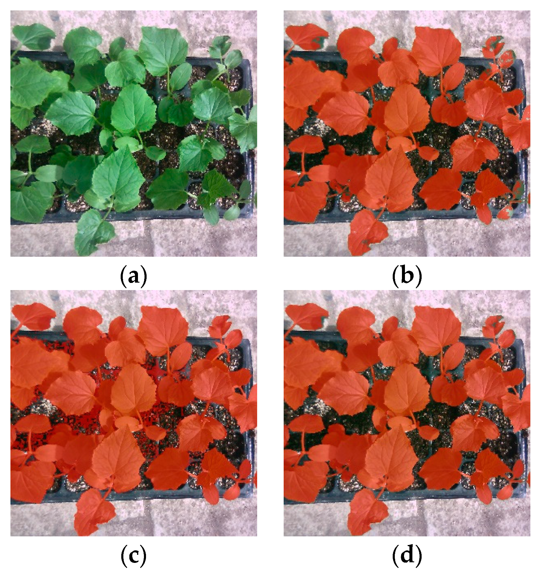
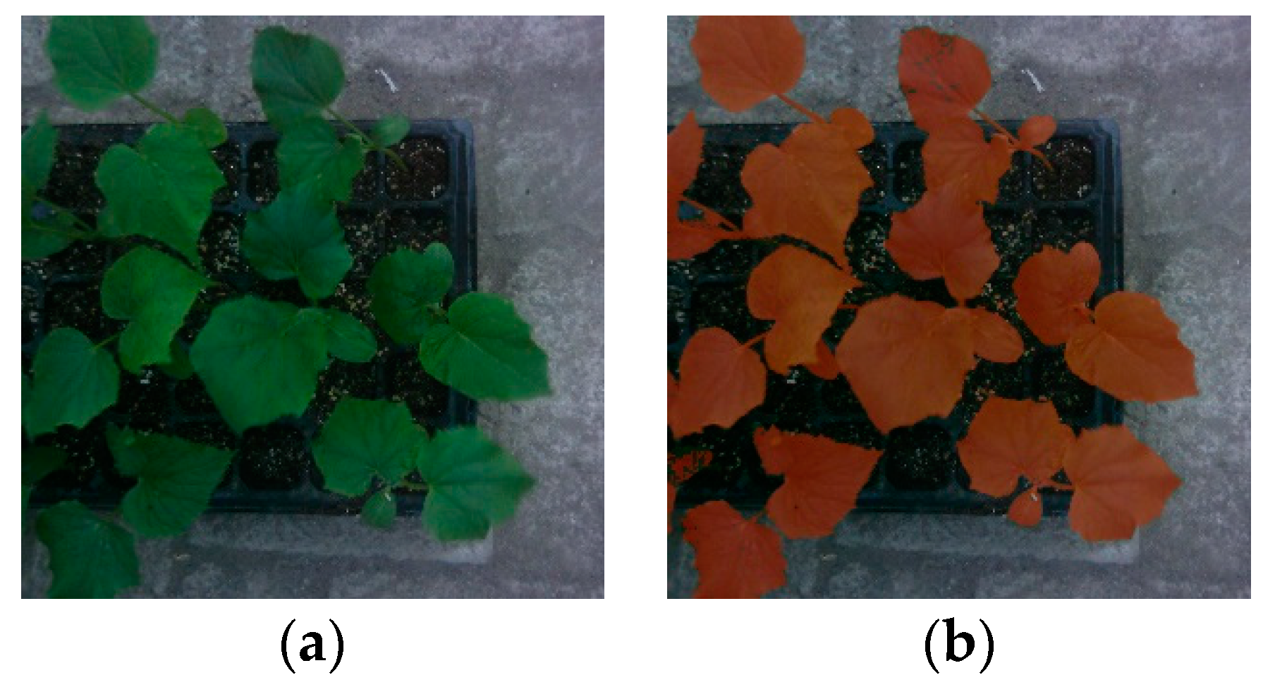
The image segmentation results obtained by selecting 2G-R-B and CIVE with good fitness from the commonly used grayscale operators and comparing them with the optimal operators in this paper are shown in Figure 11, Figure 12 and Figure 13. The figures show the effects of segmentation for different operators under three illumination conditions. A semi-transparent red mask is used to superimpose the segmentation results on the original image, which is beneficial for observing the segmentation effects.

The FPR, PRE, REC, and F1 scores for all images were calculated and averaged for the three grayscale operators under strong, weak, and normal lighting conditions, as shown in

Table 2. The average evaluation metrics of each operator under three lighting conditions.

	Strong Light (%)				Weak Light (%)				Normal Light (%)
	FPR	PRE	REC	F1	FPR	PRE	REC	F1	FPR	PRE	REC	F1
2G-R-B	0.4	97.4	89.1	91.4	1.0	96.5	91.1	93.7	0.6	96.6	92.0	94.2
CIVE	4.7	89.9	97.4	93.5	4.4	91.6	97.3	94.4	4.0	92.0	98.0	94.8
Optimal operator	0.9	96.4	93.0	94.6	1.2	96.2	92.7	94.4	1.2	95.6	95.9	95.7

.

7. Discussion

The overall segmentation effect of 2G-R-B is positive, but partial under-segmentation occurs under both strong and weak lighting conditions, as shown in Figure 11b. The over-segmentation of CIVE was found in all three lighting conditions, especially in the strong condition, where large areas of false segmentation and noise appear, and this considerably degrades the quality of the subsequent image processing. In this paper, a grayscale operator optimized by the GA is used to enhance the difference between the foreground and background in grayscale images by enhancing the foreground and suppressing the background, which ultimately enhances the effect of image segmentation. It can be seen intuitively from the segmentation results that the operator in this paper was able to segment cucumber seedlings perfectly under the three lighting conditions, preserving the shape and details of the plant with excellent adaptation to light variations.

The REC value of 2G-R-B was about 90% under different lighting conditions, with all values lower than the operator in this paper, and the lowest value was achieved under strong lighting conditions, which was 89.0%. Its FPR was also slightly lower than the optimal operator, indicating that the segmentation image of this operator is less noisy. Under the three lighting conditions, the REC of CIVE reached 97.3%, 97.3%, and 98.0%, respectively, and the FPR reached 4.3%, 4.4%, and 4.0%, respectively, which are all much higher than the other two operators, and the F1 score is higher than that of 2G-R-B. Combined with the actual segmentation results, although the segmentation precision of CIVE is elevated, the FPR value is elevated, there are segmentation problems, and it is difficult to retain the current edge information of the plant. Compared to the other two lighting conditions, the REC of the optimal operator was the lowest under the weak lighting condition, which was 92.7%. The REC values of the optimal operator were 3.9%, 1.6%, and 3.9% higher than those of 2G-R-B under the three lighting conditions, respectively. The FPR and PRE values of the optimal operator were slightly lower than those of 2G-R-B, but the F1 score was higher than that of the other two operators under the three lighting conditions, and the increase was largest under the strong lighting condition, reaching 3.2%. In regard to the F1 score, the values under strong and weak lighting conditions were lower than those under normal lighting conditions. It shows that the strong and weak lighting conditions have certain negative effects on the segmentation abilities of the three grayscale operators. On the whole, the F1 score of the operator in this paper is more stable under the three lighting conditions, and its robustness and performance are better than traditional algorithms that can achieve better segmentation, indicating that the optimal operators are more adaptable to changes in lighting conditions.

Based on the principles and experimental results, it can be inferred that the proposed algorithm has some generality and enhances the segmentation effect by enlarging the difference between the plants and the background. Therefore, the algorithm is also applicable to other plant species with different morphologies, colorimetric characteristics, and ages. Because of the algorithm’s ability to adapt to light, it should also adapt to field conditions with variable light conditions. In the future, the identification target of this algorithm may be multiple plant species, and the algorithm will simultaneously obtain the center coordinates of each plant to assist the spraying robot in completing the spraying job. Based on this method, developing mobile applications for field applications will improve the usability of the algorithm.

8. Conclusions

In this paper, a method for the quick and accurate segmentation of cucumber seedlings in seedling trays in a greenhouse environment is proposed. The RGB color space was chosen, the cucumber seedlings were identified as targets, the grayscale operator was optimized by the genetic algorithm, and then the images were segmented via the Otsu algorithm. Finally, the morphological opening and closing operations and the area-based noise filtering method were used to denoise the images. The rapid and accurate segmentation of cucumber seedlings was achieved. The segmentation effect of this approach is robust. Compared to the commonly used 2G-B-R, CIVE, and other operators, the segmentation performance of this method is significantly improved and more robust under the three lighting conditions.

This method is usually useful in solving crop image recognition problems with complex backgrounds, variable illumination, and relatively small differences between the target and background. In addition, this method is also suitable for outdoor farmland environments where lighting conditions vary widely, and the objects of image segmentation are not limited to cucumber seedlings but can be most green plants. Moreover, the algorithm does not require a large amount of computation, is simple to implement, and is highly robust for image segmentation.

However, there are some drawbacks to this method. For example, when sample collection is carried out manually, the randomness of the collected foreground and background samples is high. If the collected pixel information is not sufficient and abundant, the results of the GA will be affected, and the segmentation effect of the operator will suffer. Meanwhile, the standard images are obtained by manual segmentation, which entails certain errors and will have some impact on the experimental results.

References

- Bai, X.D.; Cao, Z.G.; Wang, Y.; Yu, Z.H.; Zhang, X.F.; Li, C.N. Crop segmentation from images by morphology modeling in the CIE L*a*b* color space. Comput. Electron. Agric. 2013, 99, 21–34. [Google Scholar] [CrossRef]
- Hamuda, E.; Glavin, M.; Jones, E. A survey of image processing techniques for plant extraction and segmentation in the field. Comput. Electron. Agric. 2016, 125, 184–199. [Google Scholar]
- Prajapati, H.B.; Shah, J.P.; Dabhi, V.K. Detection and Classification of Rice Plant Diseases. Intell. Decis. Technol. 2017, 11, 357–373. [Google Scholar] [CrossRef]
- Fountas, S.; Malounas, I.; Athanasakos, L.; Avgoustakis, I.; Espejo-Garcia, B. AI-Assisted Vision for Agricultural Robots. AgriEngineering 2022, 4, 674–694. [Google Scholar] [CrossRef]
- Guijarro, M.; Riomoros, I.; Pajares, G.; Zitinski, P. Discrete wavelets transform for improving greenness image segmentation in agricultural images. Comput. Electron. Agric. 2015, 118, 396–407. [Google Scholar]
- Castillo-Martínez, M.Á.; Gallegos-Funes, F.J.; Carvajal-Gámez, B.E.; Urriolagoitia-Sosa, G.; Rosales-Silva, A.J. Color index based thresholding method for background and foreground segmentation of plant images. Comput. Electron. Agric. 2020, 178, 105783. [Google Scholar]
- Woebbecke, D.; Meyer, G.; VonBargen, K.; Mortensen, D. Color indices for weed identification under various soil, residue, and lighting conditions. Trans. ASAE 1995, 38, 271–281. [Google Scholar]
- Meyer, G.E.; Hindman, T.W.; Lakshmi, K. Machine vision detection parameters for plant species identification. In Precision Agriculture and Biological Quality, Proceedings of SPIE; Meyer, G., DeShazer, J., Eds.; Elsevier: Bellingham, WA, USA, 1998; pp. 327–335. [Google Scholar]
- Kataoka, T.; Kaneko, T.; Okamoto, H.; Hata, S. Crop growth estimation system using machine vision. In Proceedings of the 2003 IEEE/ASME International Conference on Advanced Intelligent Mechatronics (AIM 2003), Kobe, Japan, 20–24 July 2003; Volume 2, pp. 1079–1083. [Google Scholar]
- Meyer, G.E.; Camargo-Neto, J.; Jones, D.D.; Hindman, T.W. Intensified fuzzy clusters for classifying plant, soil, and residue regions of interest from color images. Comput. Electron. Agric. 2004, 42, 161–180. [Google Scholar] [CrossRef]
- Guijarro, M.; Pajares, G.; Riomoros, I.; Herrera, P.J.; Burgos-Artizzu, X.P.; Ribeiro, A. Automatic segmentation of relevant textures in agricultural images. Comput. Electron. Agric. 2011, 75, 75–83. [Google Scholar] [CrossRef]
- Yang, W.Z.; Wang, S.L.; Zhao, X.L.; Zhang, J.S.; Feng, J.Q. Greenness identification based on HSV decision tree. Inf. Process. Agric. 2015, 2, 149–160. [Google Scholar] [CrossRef]
- Tian, K.; Li, J.H.; Zeng, J.F.; Evans, A.; Zhang, L.N. Segmentation of tomato leaf images based on adaptive clustering number of K-means algorithm. Comput. Electron. Agric. 2019, 165, 104962. [Google Scholar] [CrossRef]
- Patil, M.A.; Manohar, M. Enhanced radial basis function neural network for tomato plant disease leaf image segmentation. Ecol. Inform. 2022, 70, 101752. [Google Scholar]
- Tassis, L.M.; Tozzi de Souza, J.E.; Krohling, R.A. A deep learning approach combining instance and semantic segmentation to identify diseases and pests of coffee leaves from in-field images. Comput. Electron. Agric. 2021, 186, 106191. [Google Scholar] [CrossRef]
- Ngugi, L.C.; Abdelwahab, M.; Abo-Zahhad, M. Tomato leaf segmentation algorithms for mobile phone applications using deep learning. Comput. Electron. Agric. 2020, 178, 105788. [Google Scholar]
- Whitley, D. A genetic algorithm tutorial. Stat. Comput. 1994, 4, 65–85. [Google Scholar] [CrossRef]
- Dai, L.; Lu, H.; Hua, D.; Liu, X.; Chen, H.; Glowacz, A.; Królczyk, G.; Li, Z. A Novel Production Scheduling Approach Based on Improved Hybrid Genetic Algorithm. Sustainability 2022, 14, 11747. [Google Scholar] [CrossRef]
- Zhao, L.; Zhang, W.; Wang, W. BIM-Based Multi-Objective Optimization of Low-Carbon and Energy-Saving Buildings. Sustainability 2022, 14, 13064. [Google Scholar] [CrossRef]
- Suh, H.K.; Hofstee, J.W.; van Henten, E.J. Investigation on combinations of colour indices and threshold techniques in vegetation segmentation for volunteer potato control in sugar beet. Comput. Electron. Agric. 2020, 179, 105819. [Google Scholar]
- Otsu, N. A Threshold Selection Method from Gray-Level Histograms. IEEE Trans. Syst. Man Cybern. 1979, 9, 62–66. [Google Scholar]
- Gao, L.W.; Lin, X.H. Fully automatic segmentation method for medicinal plant leaf images in complex background. Comput. Electron. Agric. 2019, 164, 104924. [Google Scholar]
- Masland, S. Machine Learning: An Algorithmic Perspective, 2nd ed.; CRC Press: Boca Raton, FL, USA, 2015. [Google Scholar]