Multi-Stage Validation of a Solar Irradiance Model Chain: An Application at High Latitudes

Abstract

Evaluating how the sources of uncertainty in solar modelling (e.g., input parameters, developed model chain) can influence the results’ accuracy is one of the main challenges when applied at high latitudes. In this study, a multi-stage validation workflow is implemented around five main stages: data acquisition, data quality check, solar radiation modelling, photovoltaic energy modelling, and experimental validation. Different data sources such as satellite observations, numerical reanalysis, and on-site ground measurements are considered as inputs, while the outcomes from each step of the model chain (e.g., decomposition modelling, transposition modelling, photovoltaic energy modelling) are compared against observations recorded from the solar radiation network at the Norwegian University of Science and Technology (NTNU-Solarnet) in Trondheim (Norway). In the first and second validation stages, the decomposition and transposition models with measured input parameters show the best accuracy indicators, but they do not fulfill the validation criteria. Conversely, in the third validation stage, the photovoltaic energy models with on-site ground measurements as inputs are experimentally validated. In conclusion, at high latitudes, the most accurate results are obtained when monitored solar irradiation data are used instead of satellite observations and numerical reanalysis. Furthermore, the shortest model chain is preferred, with equal data sources.

1. Introduction

The interest in solar energy in Norway has steadily increased in recent years: the installed solar power capacity grew from 15 MW in 2015 to 225 MW in 2021 [1]. The slower adoption of solar energy systems in the region has come from the belief that Nordic countries have low solar energy potential compared to continental Europe [2]. However, several research studies have shown that the distribution of solar radiation throughout the year in Nordic countries is simply different from that in continental Europe. The lower number of daylight hours in winter is counterbalanced by greater sunlight availability during the summer [3,4]. The angle of the sun varies significantly throughout the year; at noon in the summer, the sun is around 50° above the horizon, while in the winter it is below 10° [5,6]. Such variability of solar radiation has an increasing impact on the built environment (e.g., daylighting, thermal and visual, solar energy production, stability of energy supply grid). To accurately estimate solar potential at high latitudes, it is, therefore, necessary to identify the most adequate model chain and solar radiation datasets to be used as input parameters.

Several studies regarding solar analysis proposed model chains that are made using a decomposition model, a transposition model, and an energy model [7,8]. The model chains implemented in [9,10] are finalized to the estimation of the energy production from photovoltaic (PV) and solar thermal (ST) panels; while, in [11,12], the authors focused on the variation in energy demand due to the passive and active solar strategies. Existing solar irradiance model chains differ in their length (i.e., the number of models in the model chain). The length of the model chain determines the results’ accuracy since each modelling stage can be an additional source of error.

Beside the model chain, input data quality is crucial for the performance of solar energy simulation models. Accurate input data are essential for the model to predict the solar potential on a surface at a specific location and to evaluate the effectiveness of solar active and passive strategies [5,13]. In this regard, the study carried out by Kenny and Fiedler [14] assessed various gridded irradiance datasets, which are commonly used in solar analyses, to identify the best for application in PV energy prediction in Germany. If the data are inaccurate, the model may produce unreliable results and may be too misleading to be used as a decision-making tool for solar system installation.

The present study aims at evaluating how the different sources of uncertainty (e.g., input solar irradiation datasets, number of steps in the model chain) can influence the accuracy of the results at high latitudes. The work is part of a wider study aiming at contributing to the transition from the currently used bidimensional solar maps [15,16], where the visualization of solar potential is limited to the rooftop surfaces and to the three-dimensional solar cadastres, where also buildings’ façades are assessed [17,18]. The need for this investigation lies in the possibility of using for the validation purpose either punctual measurements of solar irradiation or the average energy production of a PV façade/roof. On the one hand, the punctually measured solar irradiance might be not representative of the solar potential of the whole building element (i.e., placing the pyranometer at the top of the façade can underestimate the reflections from the ground). On the other hand, the average energy production required a longer model chain, which includes the energy domain in addition to the solar irradiation domain. In previous studies about the validation of solar irradiance models, one of these two parameters is often chosen for validation purposes regardless of the different associated uncertainties [19,20]. The novelty of this study is represented by the implemented multi-stage validation workflow which enables the comparative assessment of two or more solar irradiance model chains with different input parameters. Furthermore, this approach permits to quantify the accuracy of the outcomes at each stage of the model chain to answer the following research questions:

• To which extent does the length of the model chain impact the accuracy of the calculated solar irradiation quantities?
• Which input data permits better prediction of solar energy at high latitudes?

These questions will be answered in the present study, which is structured as follows. The section on materials and methods (Section 2) defines the workflow, the tools, the used datasets, the case study, the data quality filter, and the accuracy indicators; the section on results (Section 3) describes the quality filter applied to the reference observations and provides an overview of the outcomes for each validation stage; the discussions section (Section 4) presents the identified recommendations for solar modelling at high latitudes and outlines the study limitations. The study concludes with a summary of the most relevant findings and their impact on the further development of model chain and application utilization in high-latitude locations (Section 5).

2. Materials and Methods

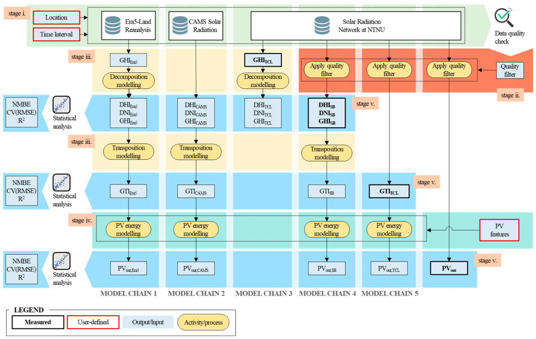
2.1. Workflow

The workflow proposed in this study is structured in five stages: (stage i) data acquisition, (stage ii) data quality check, (stage iii) solar radiation modelling, (stage iv) PV energy modelling, and (stage v) experimental validation (Figure 1). In stage i, the data regarding solar energy production, solar irradiation, and weather variables are acquired from different sources, e.g., Solar Radiation service from Copernicus Atmosphere Monitoring Service (ads.atmosphere.copernicus.eu, accessed on 30 January 2023) (CAMS), European Centre for Medium-Range Weather Forecasts (cds.climate.copernicus.eu, accessed on 30 January 2023) (ECMWF), and the solar radiation network at NTNU (NTNU-Solarnet) (see Section 2.4). Furthermore, the input parameters of this stage are the location of the case study (e.g., latitude, longitude), and the time interval (e.g., start date and end date of the analysis) to be investigated.

A Python script is created to retrieve datasets from relevant databases and merge them into a single data-frame called “solar datasets”. In particular, the Application Programming Interface (API) of the Climate Data Store (CDS) of Copernicus Europe is used to retrieve data from ECMWF; while the pvlib.iotools.get_cams function from pvlib-python package [21] enables downloading data from CAMS. The measured solar irradiation values from the installed sensors of the NTNU-Solarnet are imported manually from the .csv files.

In stage ii, data recorded by the NTNU-Solarnet is categorized based on the quality check method outlined in Section 2.5. Each datapoint is assigned a quality flag (QF), which is then utilized to screen the recorded data by excluding erroneous measurements from validation.

Stage iii and stage iv are the main steps of the solar irradiance model chain: the decomposition and the transposition modelling are included in stage iii, while stage iv focuses on the simulation of the PV energy generation outputs. The GHI is split by the decomposition model into diffuse horizontal irradiation (DHI) and direct normal irradiation (DNI). Then, the direct and the diffuse fractions are exploited by the transposition model to calculate the global tilted irradiation (GTI) (stage iii). Finally, the GTI is converted into solar energy impinging on the PV modules, and it is used to quantify the PV energy generation outputs, in stage iv. Alongside GTI, the features of the PV panel (e.g., tilt angle, azimuth angle, area, efficiency of the panel and the inverter) are defined as input parameters in this stage. Moreover, temperature-dependent losses [22] and soiling issues [23] are considered in the calculation, as described in Section 2.2. This solar irradiance model chain is applied to the solar irradiation dataset acquired during stage i. In total, up to five solar irradiance model chains, which are characterized by different lengths and input parameters, are run in parallel.

During stage v, the solar irradiation variables and the PV energy generation outputs, which are estimated in the previous stages of the model chain, are validated against measured quantities retrieved from the NTNU-Solarnet. The two datasets (i.e., calculated data, observed data) are compared in scatter plots: one graph is created for each variable to be validated. Moreover, the Normalized Mean Bias Error (NMBE), the Coefficient of Variation of the Root Mean Square Error (CV(RMSE)), and the coefficient of determination (R²) are estimated to assess the results’ accuracy.

2.2. Tools and Model Chain

A model chain consists of a sequence of model stages that perform specific tasks. The full-length model chain implemented in this study is made using a decomposition model, a transposition model, and an energy model. This model chain is flexible, and its length varies depending on the available inputs and the desired outputs. For example, if the input values are the DNI and DHI, the decomposition modelling stage is not necessary. Similarly, if the study aims at evaluating the solar irradiation impinging on a surface, the model chain can be interrupted before the energy modelling stage, giving the latter a non-requested output.

Several models are available that are well-established for hourly irradiance decomposition methods and one-minute decomposition methods [24]. These models differ in accuracy and for the predictors that are needed to estimate the diffuse fraction. In this study, the Engerer4 model is exploited to decompose the GHI into DNI and DHI. The Engerer4 model is a quasi-universal model which has been implemented by Bright and Engerer [25]. They have updated the Engerer2 [26] model by recalculating the parameters with datasets from 75 different stations worldwide. This is the most recent model from Engerer and it calculates the k_d accordingly to the equation:

$$k_d^{ENGERER4}=C+\frac{1-\mathrm{C}}{1+e^{{\beta }_0+{\beta }_1·k_t+{\beta }_2·AST+{\beta }_3·\mathsf{\theta }+{\beta }_4·\Delta k_{tc}} }+{\beta }_5·k_{de}$$

(1)

where AST is the apparent solar time, θ is the zenith angle, Δk_tc is the deviation between the clearness index for the clear sky (k_tc) and clearness index (k_t), and k_de is the proportion of k_d which depends on cloud enhancement. The C and the β-coefficients are the same as presented in [25]. Regarding the transposition models, the pvlib-python package [21], an open-source and community-supported tool that allows managing the whole solar irradiance model chain, is exploited. The Perez anisotropic model [27] is selected. It is one of the most universally exploited for building performance simulation, although other options are also available in the pvlib-python package (e.g., the isotropic model [28], the Hay–Davies model [29], and the Reindl model [30]). The Perez model splits the diffuse irradiance into different solar diffuse components (i.e., isotropic, circumsolar, horizontal brightening band), and then it estimates the amount of solar irradiance impinging on the PV modules. In particular, the total irradiance on a tilted surface is given by the following equation [27,28]:

$$I_T=I_{h,b}·R_b+I_{h,d}·\left[\left(1-F_1\right)·\left(\frac{1+\mathit{cos}\beta }{2}\right)+F_1·\frac{a}{b}+F_1·\sin \beta \right]+I_h·\rho ·\left(\frac{1-\mathit{cos}\beta }{2}\right)$$

(2)

where ${\mathrm{I}}_{\mathrm{T}}$ is the GTI, ${\mathrm{I}}_{\mathrm{h},\mathrm{b}}$ is the direct-normal component of solar irradiance on the horizontal surface, ${\mathrm{R}}_{\mathrm{b}}$ is a variable geometric factor, ${\mathrm{I}}_{\mathrm{h},\mathrm{d}}$ is the DHI, β is the surface tilt angle from the horizon, ${\mathrm{I}}_{\mathrm{h}}$ is the GHI, and $\mathsf{\rho }$ is hemispherical–hemispherical ground reflectance. The F₁ and F₂ factors, as well as the a and b terms, are computed as illustrated in Loutzenhiser et al. [27].

The solar position (i.e., solar azimuth, solar zenith, apparent solar time), which is one of the Perez model’s input parameters, is estimated with the ephemeris function included in the pvlib-python package.

Finally, the GTI, expressed in Wh/m², is used to predict the hourly energy amount generated by the PV panels (PV_out). The PV_out is calculated with the equation from the EN 15316-4-3:2017 standard:

$$P{V}_{out}=\frac{GTI·P_{pk}·f_{perf}}{I_{ref}}$$

(3)

where ${\mathrm{P}}_{\mathrm{pk}}$ is the system peak power in W at reference conditions (${\mathrm{I}}_{\mathrm{ref}}$ = 1000 W/m²). The system performance factor, ${\mathrm{f}}_{\mathrm{perf}}$, accounts for losses due to soiling (${\mathsf{\phi }}_{\mathrm{soil}}$) and temperature (${\mathsf{\phi }}_{\mathrm{temp}}$), as well as to the specific array’s configuration (${\mathsf{\phi }}_{\mathrm{array}}$) and the inverter’s efficiency (${\mathsf{\eta }}_{\mathrm{inv}}$). It is calculated according to the Norwegian technical guideline SN-NSPEK 3031:

$$f_{perf}=IAM·\left(1-\frac{{\phi }_{soil}}{100}\right)·\left(1-\frac{{\phi }_{temp}}{100}\right)·\left(1-\frac{{\phi }_{array}}{100}\right)·\frac{{\eta }_{inv}}{100}$$

(4)

where IAM is the Incident Angle Modifier. The ${\mathsf{\eta }}_{\mathrm{inv}}$ equals 96%, while the IAM is defined based on the empirical values proposed in the standard for the Trondheim location and the selected months. In particular, the IAM is 0.96, the ${\mathsf{\phi }}_{\mathrm{soil}}$ ranges between 2% and 5%, and the ${\mathsf{\phi }}_{\mathrm{array}}$ is 5.5%. Finally, the ${\mathsf{\phi }}_{\mathrm{temp}}$ depends on the cell’s temperature (${\mathrm{T}}_{\mathrm{cell}}$), and it is estimated as:

$${\phi }_{temp}={\alpha }_{temp}·\left(T_{cell}-25 °\mathrm{C}\right)$$

(5)

where ${\mathsf{\alpha }}_{\mathrm{temp}}$ is a temperature coefficient and equals 0.40% per Celsius degree.

2.3. Input Parameters

The weather data used in this work refers to Trondheim (Norway, lat. 63°25′49.76″ N). According to the Köppen Geiger classification [31], the climate of Trondheim is classified as continental sub-artic climate (Dfc), and it is moderately continental, with cold winters and mild summers. The analyses are carried out for two periods that are from 24 August 2021 to 18 December 2021 and from 4 July 2022 to 11 November 2022, respectively. The selected datasets are characterized by a time resolution ranging from one minute to one hour depending on the source.

An overview of the used datasets and their properties (i.e., data type, time resolution, spatial resolution, parameters) is presented in

Table 1. Characteristics of the datasets used in this study.

Data Source	Data Type	Timestep	Spatial Resolution	Parameters
Era5-land	Reanalysis	1 h	9 km	GHIEra5
CAMS	Satellite data	1 min	3–5 km	DHICAMS, DNICAMS, GHICAMS
Sentralbygg 1	Monitored data	1 min	point	DHISB, DNISB, GHISB
Test Cell Lab	Monitored data	5 min	point	GHITCL
Test Cell Lab	Monitored data	1 h	point	GTITCL
Test Cell Lab	Monitored data	1 h	point	PVout

. The two periods have been selected to assess the viability of the datasets to estimate solar irradiation and PV energy generation outputs during clear sky days and days characterized by overcast sky conditions. Before calculating the accuracy indicators (see Section 2.6), the datasets are resampled hourly.

Among the datasets provided by the ECMWF, the 5 generation of numerical reanalysis (Era5-Land) is selected. Era5-Land consists of a version of Era5 which is specifically developed for land applications. According to the different fields of applications, the spatial resolution of Era5-Land (9 km) is greater than the one of Era5 (around 30 km). Data covers a time horizon ranging from January 1950 to the present, and concern the main parameters related to temperature, lakes, snow, soil water, radiation and heat, evaporation, wind, pressure, and precipitation. The variables retrieved from the Copernicus Climate Data Store for the time domain of this work are the surface solar radiation downwards (corresponding to the GHI), both the temperature and the dewpoint temperature at two meters from the ground, and the surface pressure. In particular, the accumulated radiation values of Era5-Land are transformed into hourly values by subtracting the previous values within each forecast horizon.

The CAMS Solar Radiation service integrates output from the CAMS global forecasting on aerosol and ozone with detailed cloud data from geostationary satellites. The service offers historical values of GHI, DHI, and DNI (including clear and overcast sky conditions) with a one-minute time resolution from 2004 to the present. Irradiance parameters were retrieved for the two investigated periods (August–December 2021 and July–November 2022).

Alongside the reanalysis and satellite observation, the amounts of solar irradiance are also measured by sensors installed in various experimental facilities at the NTNU Gløshaugen campus. In particular, the hourly values of GHI and GTI are collected through two pyranometers installed on the rooftop of the Test Cell Lab [32], while the GHI, the DHI, and the DNI are measured through a sun tracker located at the top of the tower of the Sentralbygg 1. The sun tracker follows the sun path over the horizon to orient the pyrheliometer in the same direction as the sunrays and to keep in the shadow the pyranometer which measures the DHI. The system is completed by an unshaded pyranometer which monitors the GHI. Different time resolutions are associated with these datasets, ranging from 1 min (GHI, DNI, and DHI from the sun tracker) to 1 h (GHI and GTI from the Test Cell Lab). Finally, also the energy generation from the photovoltaic installed on the rooftop of the Test Cell Lab is monitored with a time resolution of 1 h. These timeseries, together with the solar irradiation quantities measured by the sun tracker (e.g., GHI, DHI, and DNI) and the GTI observed in the Test Cell Lab’s rooftop, represent the reference values in the experimental validation. These values are compared against the outputs collected by the different solar irradiance datasets.

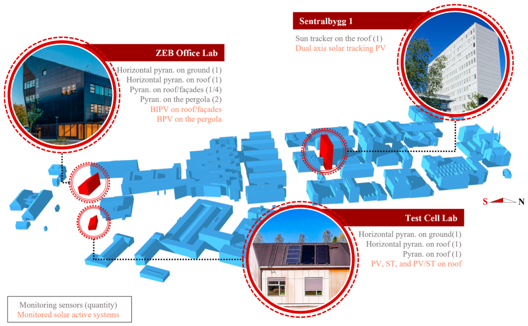
2.4. Solar Radiation Network at NTNU (NTNU-Solarnet)

The NTNU-Solarnet consists of a network of monitoring sensors and monitored solar panel systems installed in the research facilities of the NTNU Gløshaugen campus (lat. 63°25′49.76″ N, long. 10°24′16.0″ E) (Figure 2). The monitoring sensors include a sun tracker and twelve pyranometers with different orientations in space. Such an apparatus enables collecting solar irradiation data with different time resolutions (Table 1).

In particular, the SOLYS2 sun tracker (www.kippzonen.com, accessed on 30 January 2023) is located at the top of the Sentralbygg 1, and it provides measured quantities of DNI, DHI, and GHI. Up to eight second-class pyranometers are also integrated into the building envelope (four in the facades and two in the roof) and into the solar pergola of the ZEB Office Laboratory [33]. They allow measuring the GHI and the GTI on the roof (tilt angle is 40°), façades (tilt angle is 90°), and both sides of the pergola (tilt angle is 60°). Three second-class pyranometers are located in the Test Cell Lab facility. Two of them monitor the GHI at the ground and the roof level, respectively; while the third collects data regarding the plane of the tilted roof (tilt angle is 43°). The solar radiation network is completed by various solar panel systems integrated into the envelope of the ZEB Office Laboratory and in the roof of the Test Cell Lab and Sentralbygg 1 facilities.

The experimental data used in this study are collected by the sun tracker in the Sentralbygg 1 and the pyranometers in the Test Cell Lab facility. Alongside these, the monitored energy production of the polycrystalline silicon modules integrated into the rooftop of the Test Cell Lab building is used for validating the calculated PV_out. The power optimizer unites (www.solaredge.com, accessed on 30 January 2023), which are provided by the manufacturer, monitor, and collect data on the performance of each module.

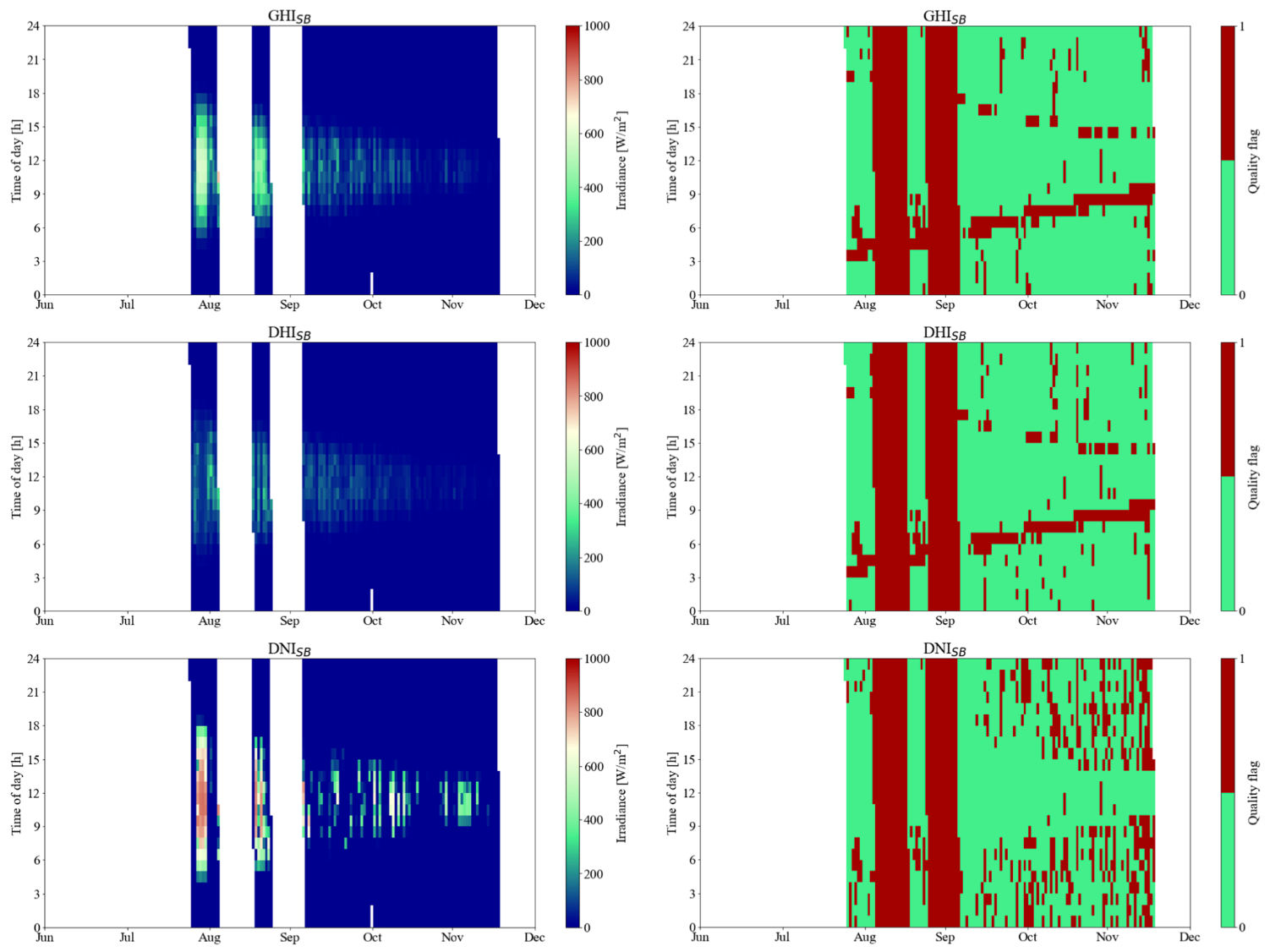
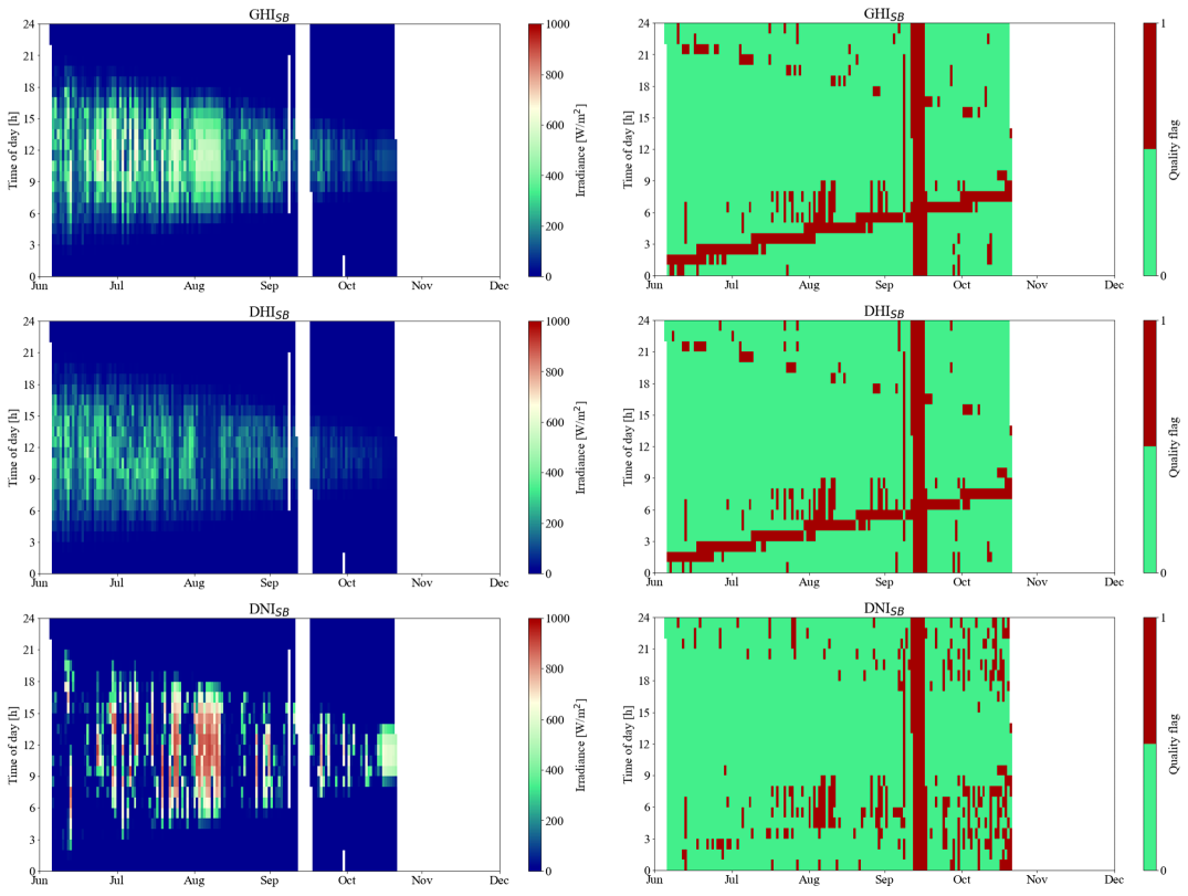
2.5. Data Quality Filter

The quality control procedure for solar irradiation datasets is not univocally defined in the literature [34,35,36]. Nonetheless, the one proposed by Long and Shi [37], and more recently used by the Baseline Surface Radiation Network (BSRN), is the most popular among authors and experts working with solar irradiation data in the last years. This protocol is also followed in this study to assign a QF to each datapoint. Data that does not comply with the following tests’ requirements are labelled as erroneous measurements (QF = 1); therefore, they are excluded from the validation process.

The procedure is structured into four tests. On the one hand, test one and test two permit the identification of the data exceeding the global physically possible limits (2)–(4) and the extremely rare limits (5)–(7). The upper and lower bounds are empirically based on atmospheric transmittance measured worldwide [37].

$$-4\mathrm{W}/{\mathrm{m}}^2<GHI<1.5·E_{0n}·{\mathit{cos}}^{1.2}\theta +100\mathrm{W}/{\mathrm{m}}^2$$

(6)

$$-4\mathrm{W}/{\mathrm{m}}^2<DHI<0.95·E_{0n}·{\mathit{cos}}^{1.2}\theta +50\mathrm{W}/{\mathrm{m}}^2$$

(7)

$$-4\mathrm{W}/{\mathrm{m}}^2<DNI<E_{0n}$$

(8)

$$-2\mathrm{W}/{\mathrm{m}}^2<GHI<1.2·E_{0n}·{\mathit{cos}}^{1.2}\theta +50\mathrm{W}/{\mathrm{m}}^2$$

(9)

$$-2\mathrm{W}/{\mathrm{m}}^2<DHI<0.75·E_{0n}·{\mathit{cos}}^{1.2}\theta +30\mathrm{W}/{\mathrm{m}}^2$$

(10)

$$-2\mathrm{W}/{\mathrm{m}}^2<DNI<0.95·E_{0n}·{\mathit{cos}}^{0.2}\theta +10\mathrm{W}/{\mathrm{m}}^2$$

(11)

where ${\mathrm{E}}_{0\mathrm{n}}$ is the direct normal irradiation outside the atmosphere and θ is the zenith angle. On the other hand, test three and test four allow for detecting issues with the measurement equipment. In test three, the deviation of the observed GHI from the sum of the direct horizontal irradiance (BHI) and the DHI is assessed (8). This should be lower than 8% for θ smaller than 75°, and lower than 15% when θ ranges between 75° and 93°. Finally, the diffuse ratio (k_d) is evaluated in test four (9). However, when the measured or calculated GHI is less than 50 W/m² or the θ is smaller than 93°, the last two tests are not possible.

$$\left|\frac{GHI}{DHI+BHI}\right|<\left\{\begin{array}{c}1.08 if \theta \le 75° and DHI+BHI>50\mathrm{W}/{\mathrm{m}}^2\\ 1.15 if 75°<\theta <93° and DHI+BHI>50\mathrm{W}/{\mathrm{m}}^2\\ N/A if DHI+BHI<50\mathrm{W}/{\mathrm{m}}^2\end{array}\right.$$

(12)

$$k_d<\left\{\begin{array}{c}1.05 if \theta \le 75° and DHI+BHI>50\mathrm{W}/{\mathrm{m}}^2\\ 1.10 if 75°<\theta <93° and DHI+BHI>50\mathrm{W}/{\mathrm{m}}^2\\ N/A if DHI+BHI<50\mathrm{W}/{\mathrm{m}}^2\end{array}\right.$$

(13)

2.6. Statistical Indicators

Several studies suggested performance indicators that can be used in radiation models for validation purposes [38,39]. Among those, three statistical indicators were chosen: the NMBE, the CV(RMSE), and the R². The NMBE consists of the normalized average of the errors of a sample space, thus allowing comparative analyses among different models. Positive values mean that the numerical model tends to under-predict the measured parameter, and negative values indicate an overestimation. It is worth highlighting that the use of NMBE alone is not recommended since this index can be subject to cancellation errors.

The CV(RMSE) measures the variability of the errors between observed and simulated values. The CV(RMSE) is not subject to cancellation errors; thus, the AHSRAE Guidelines [40] couple it with the NMBE index to verify the models’ accuracy.

The R² index provides information on how close the simulated values are to the regression line of the observed values. It ranges from 0 to 1, where 0 indicates a complete mismatch between observed and simulated values and 1 is a perfect match.

When it comes to the calibration of the numerical model, the criteria provided by the ASHRAE Guideline 14 are adopted (

Table 2. Validation criteria provided by the ASHRAE Guideline 14.

Calibration Criteria
NMBE	<±10%
CV(RMSE)	<30%
Model recommendation
R2	>0.75

).

3. Results

3.1. Data Quality Check

The quality check of the solar irradiation data recorded by the sun tracker installed in the Sentralbygg 1 at Gløshaugen campus during the two investigated periods (i.e., August–December 2021 and July–November 2022) is performed by assigning a QF to each observation. Following this, the datapoints suitable to be used in the validation process (QF = 0) are filtered out.

An overview of the recorded data and the corresponding QFs is presented in Figure 3 and Figure 4. The visual inspection of the diagrams suggests that a high level of inaccuracy (QF = 1) is mostly associated (i) with low solar irradiation amounts and (ii) with those values that have been measured during particularly overcast sky conditions. It is worth mentioning that the monitoring system is found to be less accurate during sunrise hours than during sunset hours. Furthermore, more datapoints with QF = 1 are present in DNI measurements compared to GHI and DHI measurements, particularly from September to December.

3.2. Multi-Stage Experimental Validation

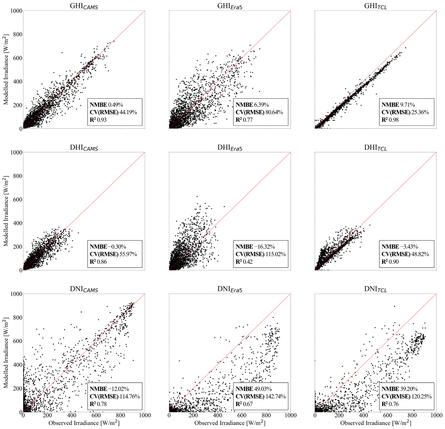
3.2.1. Decomposition Modelling

In this section, the validation of the first step of the model chain (i.e., decomposition modelling) is performed against the experimental data collected by the sun tracker of the NTNU-Solarnet.

The outcomes from the decomposition model described in Section 2.2 are reported in the scatter plots in Figure 5. In particular, the observed GHI_SB, DHI_SB, and DNI_SB amounts are shown against the GHI, DHI, and DNI outputs which derive from the Test Cell Lab, CAMS, and Era5-Land. It is worth highlighting that only the values that satisfy the data quality check requirements are considered in the validation process.

These results enable some preliminary considerations. Firstly, the Test Cell Lab and CAMS datasets can predict both the GHI and the DHI better than the Era5-Land reanalysis. Secondly, none of the datasets provides reliable outcomes when calculating the DNI. In particular, the DNI values that are modelled on GHI_Era5 and GHI_TCL are usually lower than the observed quantities. Thirdly, the DNI_CAMS dataset presents some null values during the hours characterized by DNI_SB different from zero, as can be seen by the point cloud adjacent to the y-axis (Figure 5).

The accuracy indicators calculated for the three datasets during the first validation stage confirmed such observations (Figure 5). The decomposition model with GHI_TCL as input parameter shows NMBE values of 9.71%, −3.43%, and 39.20% for GHI, DHI, and DNI estimations, respectively. Beside this, the CV(RMSE) ranges from 25.36% (GHI) to 48.82% (DHI), and to 120.25% (DNI), while the R² is always higher than 0.90, except for the DNI (0.76). These are the accuracy indicators corresponding to the best performance, while the worst results are obtained when Era5-Land reanalysis is used. Satellite observations (i.e., CAMS) were found to be accurate in estimating GHI and DHI, but not DNI. None of the models can be validated for all solar irradiation variables (i.e., GHI, DHI, DNI) according to the adopted validation criteria. Nonetheless, the GHI outcomes from the decomposition model exploiting solar irradiation data from the Test Cell Lab are validated.

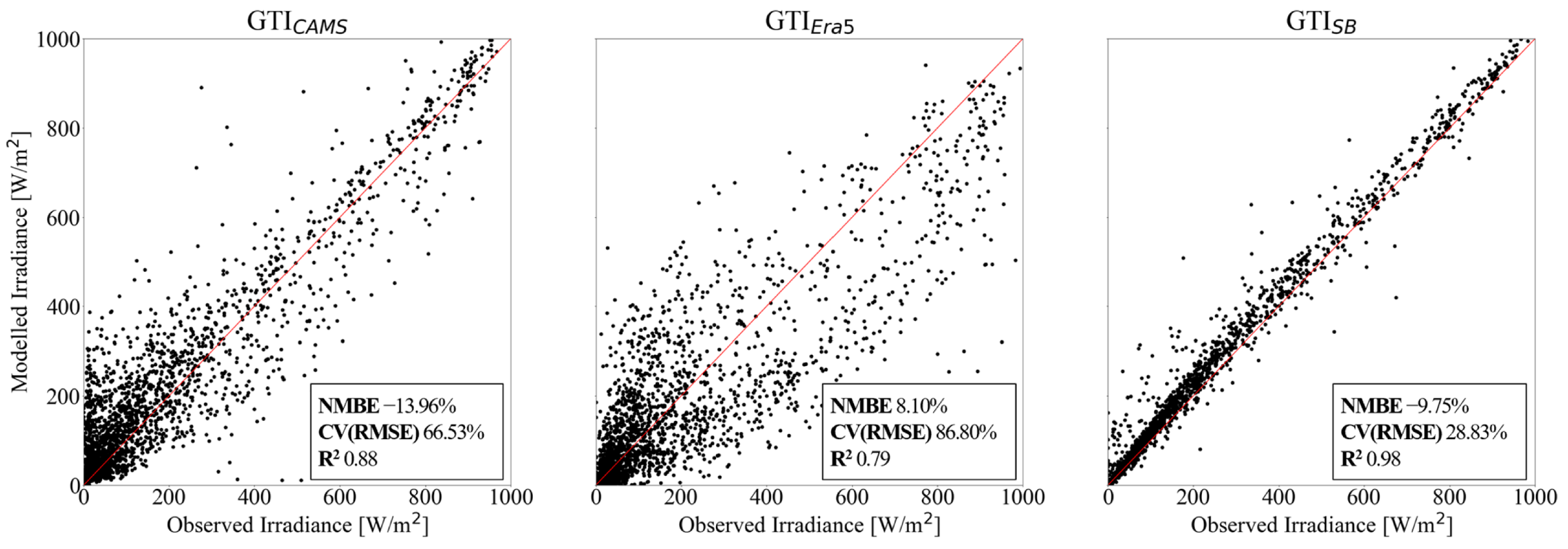
3.2.2. Transposition Modelling

This section focuses on transposition modelling, presenting the second validation stage against the observations from the pyranometer integrated into the tilted rooftop of the Test Cell Lab. The results from the transposition model are presented in the scatter plots in Figure 6, where the observed GTI_TCL is plotted against the GTI_CAMS, GTI_Era5, and GTI_SB, respectively.

The visual inspection of the plots highlights the high accuracy of the GTI amounts that result from the transposition of the DHI_SB and DNI_SB. On-site ground measurements are more accurate than both satellite observations and numerical reanalysis when it comes to calculating GTI at high-latitude locations.

Such a preliminary consideration is confirmed by the accuracy indicators reported in Figure 6. The transposition model is found to perform best when DHI_SB and DNI_SB are used as input parameters, resulting in an NMBE of −9.75%, a CV(RMSE) of 28.83%, and an R² of 0.98. The worst results are obtained when solar irradiation data from Era5-Land are used as inputs. The validation criteria described in the ASHRAE Handbook (Table 2) are satisfied only by the transposition model with DHI_SB and DNI_SB as inputs.

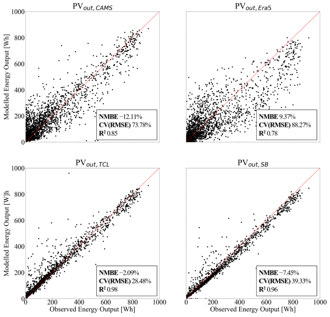
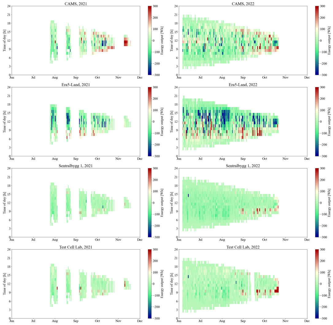
3.2.3. PV Energy Generation Modelling

The PV energy generation modelling represents the final step of the proposed model chain in this study. In particular, the modelled PV energy generation quantities (e.g., PV_out,Era5, PV_out,CAMS, PV_out,SB, PV_out,TCL) are here validated against the data acquired in the Test Cell Lab during the two investigated periods (Figure 7).

The visualization of the results in Figure 7 shows that the PV_out amounts estimated from on-site ground measurements of solar irradiance are the most accurate, regardless of the measured solar irradiance variable (i.e., GTI or DHI and DNI). This is also demonstrated by the accuracy indicators. In fact, the calculated NMBE values equal 9.37% (PV_out,Era5), −12.11% (PV_out,CAMS), −7.45% (PV_out,SB), and −2.09% (PV_out,TCL), while the estimated CV(RMSE) values are 88.27% (PV_out,Era5), 73.78% (PV_out,CAMS), 39.33% (PV_out,SB), and 28.84% (PV_out,TCL). Finally, the R² ranges between 0.78 (PV_out,Era5) and 0.98 (PV_out,TCL). According to the validation criteria applied in this study (see Section 2.6), only the PV energy models exploiting the on-site ground measurements of GTI from the Test Cell Lab as input can be experimentally validated. Nonetheless, the PV energy outputs modeled from DHI_SB and DNI_SB are close to the requirements (i.e., CV(RMSE) is around 10% higher than the 30% threshold).

4. Discussion

4.1. Recommendations for Solar Irradiation Modelling at High Latitudes

The multi-stage validation process performed in this study allowed identifying some recommendations regarding the length of the model chain and the number of steps, as well as the input data for solar irradiation analysis at high latitudes. In particular, the experimental validation of the decomposition, the transposition, and the PV energy generation models highlight the importance of implementing the shortest possible model chain. In fact, the values of the GTI estimated from the GHI_Era5 (i.e., through decomposition and transposition models), are found to be less accurate than the GTI quantities calculated by transposing the DHI_CAMS and the DNI_CAMS. The direct and diffuse fractions from CAMS can also predict the PV_out more precisely if compared to the GHI data retrieved from the Era5-Land dataset. This is confirmed by the residues calculated between the observed and the modelled PV_out quantities, which show a higher number of anomalies (i.e., hours characterized by significant variation from the reference value) in Era5-Land than in CAMS (Figure 8).

When on-site ground measurements (i.e., Sentralbygg 1, Test Cell Lab) are exploited, the length of the model chain impacts the accuracy of results in a similar way, as demonstrated by the indicators calculated for the PV_out,SB and the PV_out,TCL. In this case, the results from the model chains using GTI_TCL as input are characterized by almost the highest level of accuracy.

Regarding the input data, the outcomes from the multi-stage validation process demonstrated that on-site ground measurements are always leading to more accurate estimations. In fact, the GHI_TCL in the first validation stage (i.e., decomposition modelling), the DHI_SB and the DNI_SB in the second validation stage (i.e., transposition modelling), and both the GTI_TCL and the GTI_SB in the third validation stage (i.e., PV energy modelling) showed the highest accuracy. Therefore, the use of datasets from on-site ground measurements should be always prioritized when performing solar irradiation analyses.

Finally, the following recommendations about solar irradiation modelling at high latitudes are identified:

• When available, solar radiation data from a monitoring apparatus (e.g., sun tracker, pyranometer, weather station) should be prioritized despite the length of the model chain.
• With equal data sources (i.e., all data are from on-site ground measurements), the shortest possible model chain should be implemented.
• Measuring GTI is a valid option since it combines the short model chain with the low costs of the monitoring sensor (i.e., pyranometer), but it requires the installation of a high number of sensors (i.e., one sensor for each orientation).

4.2. Limitations of the Study

In this section, the limitations of this study are outlined and commented upon. Firstly, the two selected time intervals are not covering the whole year, with some months (and seasons) which are not represented. Therefore, the results might be affected by the specific weather conditions of the selected period of the year (i.e., between July and December). However, these datasets are representative of different possible sky conditions: clear sky conditions are prevalently observed between July and September, and overcast conditions are more frequent between October and December. In addition, the use of datasets from two years allowed to mitigate the impact of singularities by increasing the number of data points.

Secondly, the use of only one combination of decomposition and transposition models can limit the reliability of the results. In fact, the use of more effective decomposition or transposition models could lead to lower accuracy indicators for those model chains with GHI or DNI and DHI as input parameters. On the contrary, using a more efficient PV energy model would have had a lower impact on the results since it is applied to every investigated dataset.

Thirdly, the use of a data quality check scheme that is not specifically implemented for high-latitude applications might result in the erroneous exclusion of correct datapoints and vice versa. Applying a quality check scheme which is developed for this case study would have resulted in more accurate filtering. However, investigating methods to ensure high-quality data is not the core of this research; therefore, a data quality check scheme, which is commonly used and universally recognized as valid by experts in solar radiation modelling, has been exploited.

5. Conclusions

In this study, a multi-stage validation of the solar irradiation model chain is performed. The outcomes from the solar irradiance decomposition and transposition models and the PV energy generation model are validated against experimental data retrieved from the NTNU-Solarnet. A data quality filter is applied to ensure the quality of the reference datasets. Different data sources (e.g., satellite observations, numerical reanalysis, on-site ground measurements) are considered as input in the model chain to assess how the length of the model chain and the selection of the data source can impact the accuracy of the results.

A summary of the main findings is here presented:

• In the first validation stage, the decomposition model with GHI_TCL as the input parameter shows the best accuracy indicators, but it cannot reliably estimate DNI.
• None of the selected data sources for decomposition modelling permits accurately estimating the DNI at high latitudes.
• In the second validation stage, the transposition model using the DHI_SB and DNI_SB as inputs fulfills the validation criteria.
• In the third validation stage, only the PV energy generation models exploiting on-site ground measurements of GTI (i.e., GTI_TCL) as input parameters can be experimentally validated.

In conclusion, on-site ground-measured solar irradiation data are found to lead always to more accurate results than both satellite observations and numerical reanalysis, despite the length of the model chain. However, with equal data sources (i.e., all data are from on-site ground measurements), the shortest model chain is to be preferred.

Future developments of this research study concern:

• Applying the workflow hereby proposed to other data sources as well as to other locations, at high latitudes.
• Investigating the impact on the accuracy of the results of the model which is chosen in each stage of the model chain (e.g., irradiance decomposition, irradiance transposition, PV energy generation estimation).
• Performing a sensitivity analysis on the results by varying the tilt angle and the azimuth of the PV panel.

References

1. Statista Solar Energy Capacity in Norway from 2010 to 2021. Available online: https://www.statista.com/statistics/1165971/total-solar-power-capacity-in-norway/ (accessed on 30 January 2023).
2. Formolli, M.; Lobaccaro, G.; Kanters, J. Solar Energy in the Nordic Built Environment: Challenges, Opportunities and Barriers. Energies 2021, 14, 8410. [Google Scholar] [CrossRef]
3. Good, C.S.; Lobaccaro, G.; Hårklau, S. Optimization of Solar Energy Potential for Buildings in Urban Areas—A Norwegian Case Study. Energy Procedia 2014, 58, 166–171. [Google Scholar] [CrossRef]
4. Babar, B.; Luppino, L.T.; Boström, T.; Anfinsen, S.N. Random Forest Regression for Improved Mapping of Solar Irradiance at High Latitudes. Sol. Energy 2020, 198, 81–92. [Google Scholar] [CrossRef]
5. Lobaccaro, G.; Carlucci, S.; Croce, S.; Paparella, R.; Finocchiaro, L. Boosting Solar Accessibility and Potential of Urban Districts in the Nordic Climate: A Case Study in Trondheim. Sol. Energy 2017, 149, 347–369. [Google Scholar] [CrossRef]
6. Manni, M.; Lobaccaro, G.; Goia, F.; Nicolini, A. An Inverse Approach to Identify Selective Angular Properties of Retro-Reflective Materials for Urban Heat Island Mitigation. Sol. Energy 2018, 176, 194–210. [Google Scholar] [CrossRef]
7. Lorenz, E.; Heinemann, D. Prediction of Solar Irradiance and Photovoltaic Power. Compr. Renew. Energy 2012, 1, 239–292. [Google Scholar] [CrossRef]
8. Gueymard, C.A.; Ruiz-Arias, J.A. Extensive Worldwide Validation and Climate Sensitivity Analysis of Direct Irradiance Predictions from 1-Min Global Irradiance. Sol. Energy 2016, 128, 1–30. [Google Scholar] [CrossRef]
9. Vinod; Kumar, R.; Singh, S.K. Solar Photovoltaic Modeling and Simulation: As a Renewable Energy Solution. Energy Rep. 2018, 4, 701–712. [Google Scholar] [CrossRef]
10. Taki, M.; Rohani, A.; Rahmati-Joneidabad, M. Solar Thermal Simulation and Applications in Greenhouse. Inf. Process. Agric. 2018, 5, 83–113. [Google Scholar] [CrossRef]
11. Manni, M.; Bonamente, E.; Lobaccaro, G.; Goia, F.; Nicolini, A.; Bozonnet, E.; Rossi, F. Development and Validation of a Monte Carlo-Based Numerical Model for Solar Analyses in Urban Canyon Configurations. Build. Environ. 2020, 170, 106638. [Google Scholar] [CrossRef]
12. Naji, S.; Aye, L.; Noguchi, M. Multi-Objective Optimisations of Envelope Components for a Prefabricated House in Six Climate Zones. Appl. Energy 2021, 282, 116012. [Google Scholar] [CrossRef]
13. Luoma, J.; Kleissl, J.; Murray, K. Optimal Inverter Sizing Considering Cloud Enhancement. Sol. Energy 2012, 86, 421–429. [Google Scholar] [CrossRef]
14. Kenny, D.; Fiedler, S. Which Gridded Irradiance Data Is Best for Modelling Photovoltaic Power Production in Germany? Sol. Energy 2022, 232, 444–458. [Google Scholar] [CrossRef]
15. Brito, M.C.; Gomes, N.; Santos, T.; Tenedório, J.A. Photovoltaic Potential in a Lisbon Suburb Using LiDAR Data. Sol. Energy 2012, 86, 283–288. [Google Scholar] [CrossRef]
16. Desthieux, G.; Carneiro, C.; Susini, A.; Abdennadher, N.; Boulmier, A.; Dubois, A.; Camponovo, R.; Beni, D.; Bach, M.; Leverington, P.; et al. Solar Cadaster of Geneva: A Decision Support System for Sustainable Energy Management BT—From Science to Society; Otjacques, B., Hitzelberger, P., Naumann, S., Wohlgemuth, V., Eds.; Springer International Publishing: Cham, Switzerland, 2018; pp. 129–137. [Google Scholar]
17. Brito, M.C. Assessing the Impact of Photovoltaics on Rooftops and Facades in the Urban Micro-Climate. Energies 2020, 13, 2717. [Google Scholar] [CrossRef]
18. Desthieux, G.; Carneiro, C.; Camponovo, R.; Ineichen, P.; Morello, E.; Boulmier, A.; Abdennadher, N.; Dervey, S.; Ellert, C. Solar Energy Potential Assessment on Rooftops and Facades in Large Built Environments Based on LiDAR Data, Image Processing, and Cloud Computing. Methodological Background, Application, and Validation in Geneva (Solar Cadaster). Front. Built Environ. 2018, 4, 14. [Google Scholar] [CrossRef]
19. Behar, O.; Khellaf, A.; Mohammedi, K. Comparison of Solar Radiation Models and Their Validation under Algerian Climate—The Case of Direct Irradiance. Energy Convers. Manag. 2015, 98, 236–251. [Google Scholar] [CrossRef]
20. Böök, H.; Poikonen, A.; Aarva, A.; Mielonen, T.; Pitkänen, M.R.A.; Lindfors, A.V. Photovoltaic System Modeling: A Validation Study at High Latitudes with Implementation of a Novel DNI Quality Control Method. Sol. Energy 2020, 204, 316–329. [Google Scholar] [CrossRef]
21. Holmgren, W.F.; Hansen, C.W.; Mikofski, M.A. PVlib Python: A Python Package for Modeling Solar Energy Systems. J. Open Source Softw. 2018, 3, 884. [Google Scholar] [CrossRef]
22. Tina, G.M.; Scavo, F.B.; Gagliano, A. Multilayer Thermal Model for Evaluating the Performances of Monofacial and Bifacial Photovoltaic Modules. IEEE J. Photovolt. 2020, 10, 1035–1043. [Google Scholar] [CrossRef]
23. Cordero, R.R.; Damiani, A.; Laroze, D.; MacDonell, S.; Jorquera, J.; Sepúlveda, E.; Feron, S.; Llanillo, P.; Labbe, F.; Carrasco, J.; et al. Effects of Soiling on Photovoltaic (PV) Modules in the Atacama Desert. Sci. Rep. 2018, 8, 13943. [Google Scholar] [CrossRef] [PubMed]
24. Yang, D. Estimating 1-Min Beam and Diffuse Irradiance from the Global Irradiance: A Review and an Extensive Worldwide Comparison of Latest Separation Models at 126 Stations. Renew. Sustain. Energy Rev. 2022, 159, 112195. [Google Scholar] [CrossRef]
25. Bright, J.M.; Engerer, N.A. Engerer2: Global Re-Parameterisation, Update, and Validation of an Irradiance Separation Model at Different Temporal Resolutions. J. Renew. Sustain. Energy 2019, 11, 33701. [Google Scholar] [CrossRef]
26. Engerer, N.A. Minute Resolution Estimates of the Diffuse Fraction of Global Irradiance for Southeastern Australia. Sol. Energy 2015, 116, 215–237. [Google Scholar] [CrossRef]
27. Perez, R.; Ineichen, P.; Seals, R.; Michalsky, J.; Stewart, R. Modeling Daylight Availability and Irradiance Components from Direct and Global Irradiance. Sol. Energy 1990, 44, 271–289. [Google Scholar] [CrossRef]
28. Loutzenhiser, P.G.; Manz, H.; Felsmann, C.; Strachan, P.A.; Frank, T.; Maxwell, G.M. Empirical Validation of Models to Compute Solar Irradiance on Inclined Surfaces for Building Energy Simulation. Sol. Energy 2007, 81, 254–267. [Google Scholar] [CrossRef]
29. Hay, J.E. Calculating Solar Radiation for Inclined Surfaces: Practical Approaches. Renew. Energy 1993, 3, 373–380. [Google Scholar] [CrossRef]
30. Reindl, D.T.; Beckman, W.A.; Duffie, J.A. Diffuse Fraction Correlations. Sol. Energy 1990, 45, 1–7. [Google Scholar] [CrossRef]
31. Manni, M.; Failla, M.C.; Nocente, A.; Lobaccaro, G.; Jelle, B.P. The Influence of Icephobic Nanomaterial Coatings on Solar Cell Panels at High Latitudes. Sol. Energy 2022, 248, 76–87. [Google Scholar] [CrossRef]
32. Goia, F.; Schlemminger, C.; Gustavsen, A. The ZEB Test Cell Laboratory. A Facility for Characterization of Building Envelope Systems under Real Outdoor Conditions. Energy Procedia 2017, 132, 531–536. [Google Scholar] [CrossRef]
33. Nocente, A.; Time, B.; Mathisen, H.M.; Kvande, T.; Gustavsen, A. The ZEB Laboratory: The Development of a Research Tool for Future Climate Adapted Zero Emission Buildings. J. Phys. Conf. Ser. 2021, 2069, 12109. [Google Scholar] [CrossRef]
34. Yang, D.; Boland, J. Satellite-Augmented Diffuse Solar Radiation Separation Models. J. Renew. Sustain. Energy 2019, 11, 23705. [Google Scholar] [CrossRef]
35. Starke, A.R.; Lemos, L.F.L.; Barni, C.M.; Machado, R.D.; Cardemil, J.M.; Boland, J.; Colle, S. Assessing One-Minute Diffuse Fraction Models Based on Worldwide Climate Features. Renew. Energy 2021, 177, 700–714. [Google Scholar] [CrossRef]
36. Yang, D.; Yagli, G.M.; Quan, H. Quality Control for Solar Irradiance Data. In Proceedings of the 2018 IEEE Innovative Smart Grid Technologies—Asia (ISGT Asia), Singapore, 22–25 May 2018; pp. 208–213. [Google Scholar]
37. Long, C.N.; Shi, Y. An Automated Quality Assessment and Control Algorithm for Surface Radiation Measurements. Open Atmos. Sci. J. 2008, 2, 23–37. [Google Scholar] [CrossRef]
38. Gueymard, C.A. A Review of Validation Methodologies and Statistical Performance Indicators for Modeled Solar Radiation Data: Towards a Better Bankability of Solar Projects. Renew. Sustain. Energy Rev. 2014, 39, 1024–1034. [Google Scholar] [CrossRef]
39. Taylor, K.E. Summarizing Multiple Aspects of Model Performance in a Single Diagram. J. Geophys. Res. Atmos. 2001, 106, 7183–7192. [Google Scholar] [CrossRef]
40. ASHRAE. Guideline 14-2002, Measurement of Energy and Demand Savings; ASHRAE: Atlanta, GA, USA, 2002. [Google Scholar]
Figure 1. Overview of the workflow followed in this study. The five stages (e.g., data acquisition, data quality check, solar radiation modelling, PV energy modelling, experimental validation) are highlighted with different colors, while block typologies (e.g., measured value, user-defined value, output/input, activity/process) are reported at the bottom.
Sustainability 15 02938 g001
Figure 2. Spatial distribution within the NTNU-Solarnet of the monitoring sensors, e.g., horizontally mounted and tilted pyranometers, sun tracker, and the monitored solar active systems, e.g., photovoltaic (PV), building-integrated PV (BIPV), bifacial PV (BPV), solar thermal (ST), hybrid ST/PV, and dual axis solar tracking PV. The experimental facilities of the NTNU-Solarnet that are considered in this study are the Test Cell Lab and the Sentralbygg 1.
Sustainability 15 02938 g002
Figure 3. Overview of the solar irradiation data (e.g., GHISB, DHISB, DNISB) recorded in 2021 by the sun tracker in the Sentralbygg 1, and the corresponding quality flags: a value of 1 is assigned to measurements with a high level of inaccuracy.
Sustainability 15 02938 g003
Figure 4. Overview of the solar irradiation data (e.g., GHISB, DHISB, DNISB) recorded in 2022 by the sun tracker in the Sentralbygg 1, and the corresponding quality flags: a value of 1 is assigned to measurements with a high level of inaccuracy.
Sustainability 15 02938 g004
Figure 5. Observed GHI, DHI, and DNI and modelled GHI, DHI, and DNI from CAMS, Era5-Land, and Test Cell Lab datasets.
Sustainability 15 02938 g005
Figure 6. Observed GTI and modelled GTI from CAMS, Era5-Land, and Sentralbygg 1 datasets.
Sustainability 15 02938 g006
Figure 7. Observed PVout and modelled PVout from CAMS, Era5-Land, Sentralbygg 1, and Test Cell Lab datasets.
Sustainability 15 02938 g007
Figure 8. Residues between the PVout estimated using datasets from CAMS, Era5, Sentralbygg 1, and Test Cell Lab data and the monitored PVout. Data from 2021 are reported on the left, while data from 2022 are on the right.
Sustainability 15 02938 g008