Operation Optimization Method of Distribution Network with Wind Turbine and Photovoltaic Considering Clustering and Energy Storage

Abstract

The problem of distribution network operation optimization is diversified and uncertain. In order to solve this problem, this paper proposes a method of distribution network operation optimization considering wind-solar clustering, which includes source load and storage. Taking the total operating cost as the objective function, it includes network loss cost, unit operating cost, and considers a variety of constraints such as energy storage device constraints and demand response constraints. This paper aims to optimize the operation according to different wind-solar clustering scenes to improve the economy of distribution network. Taking the 365-day wind-solar output curves as the research object, K-means clustering is carried out, and the best k value is obtained by elbow rule. The second-order cone programming method and solver are used to solve the optimization model of each typical scenario, and the operation optimization analysis of each typical scenario obtained by clustering is carried out. Taking IEEE33 system and local 365-day wind-solar units output scenes as examples, the period is 24 h, which verifies the effectiveness of the proposed method. The proposed method has guiding significance for the operation optimization of distribution network.

1. Introduction

The distribution network operation optimization (DNOO) problem is essentially a multivariate and uncertain problem [1]. With the construction of new energy power system, the transformation of energy is unstoppable, and the status of new energy power generation (especially photovoltaic and wind power) in the power system is gradually rising [2,3,4,5], which increases the difficulty of distribution network operation optimization [6,7]. Because large-scale wind and solar time series data will bring high time complexity to the optimization program, it is necessary to determine the typical scene of wind and scenery. However, the annual wind-solar power output curves are repetitive to some extent, so it is not necessary to study the wind-solar power output data of 365 days in the whole year. Therefore, cluster analysis is carried out on them first [8], and then the operation optimization analysis is carried out for the wind-solar output of each typical day after clustering.

Scholars within China and abroad have made some achievements in DNOO research. Reference [9] simulated wind power output, clustered typical discrete scenes, and put forward a distributed optimization model of AC/DC hybrid distribution network considering the uncertainty of wind power. Reference [10] established the optimal operation model of distribution network with high permeability distributed generation based on SOP and switchable capacitors, and solved it by the multi-objective optimization algorithm of non-dominated sorting method. Reference [11] put forward a three-level robust planning-operation joint optimization model of distribution network considering high photovoltaic permeability, which was solved by three-level decomposition algorithm. Reference [12] had established an integrated distribution system operation optimization model, which took the minimum operation cost as the objective function and used the mixed integer second-order cone programming method to solve it. Reference [13] put forward a partial optimization model of double-layer random operation of distribution network-natural gas combined system considering scenario clustering, which improved the adaptability of operation scheme to wind power fluctuation from multiple time scales, but did not consider the fluctuation of photovoltaic. At present, there is no research literature on distribution network operation optimization considering wind power and photovoltaic clustering, so further research is still needed.

Aiming at the DNOO problem with multiple uncertainties, this paper determines the k value according to the elbow method, clusters the annual wind and solar data into k typical scenes, and obtains the power of each typical solar and wind turbine. Then, the optimization model of distribution network operation with source, load and storage is established, and the models in various typical scenes are solved by the second-order cone method and cplex solver. The main contributions of this work are outlined as follows:

(1)

Based on K-means clustering method, the annual wind-solar output curves of a certain area are divided, and typical scenes are determined for subsequent optimization;

(2)

A model solving method based on the second-order cone programming method has been proposed to obtain the optimal solution in a short time;

(3)

Based on the proposed distribution network operation optimization method considering wind-solar clustering, the IEEE33 system in a certain area is optimized and analyzed, which reduces the total operation cost and voltage deviation to the greatest extent;

2. Determination of Typical Scenes Based on K-Means Clustering

Scene Analysis (SA) is an effective way to analyze the uncertainty of power system by constructing typical scenes [14,15]. It can solve the problem of power system operation optimization with renewable energy.

2.1. Scene Cluster Analysis

Based on K-means clustering algorithm, k sampling points are randomly selected from the sampling set of wind and solar power data as wind and solar cluster centers, and the distances between all sampling points and these k cluster centers are calculated. For each sample, it is divided into the same class as the nearest cluster center, and a new cluster center is calculated.

The steps of landscape cluster analysis can be roughly divided into the following steps:

Step (1) Selection of k value

The choice of k can be determined by observation or according to the elbow rule. Because the naked eye observation varies from person to person, the elbow method is relatively more suitable for high-dimensional sample data.

Step (2) Distance measurement

Divide the sampling points into the class closest to the cluster center. This process requires the nearest neighbor measurement strategy, which usually adopts the Euclidean distance, and its calculation formula is as follows:

$$d(x,y)=\sqrt{{(x_1-y_1)}^2+\cdots +{(x_n-y_n)}^2}=\sqrt{{\displaystyle {\sum }_{i=1}^n{(x_i-y_i)}^2}}$$

(1)

Step (3) Calculation of new centroid

For the k classes generated after classification, the point with the smallest mean distance to other points in the class is calculated as the centroid.

Step (4) Whether or not stop K-means

Repeat step (2) and (3) until the center of mass does not change or the maximum number of iterations of a given cycle is reached, and then the clustering process will stop.

Step (5) Determine k typical scenarios.

2.2. Elbow Rule Determines k Value

The key index of elbow method is Sum of squares for error (SSE):

$$SSE={{\displaystyle {\sum }_{i=1}^k{\displaystyle {\sum }_{p\in C_i}\left|p-m_i\right|}}}^2$$

(2)

Using SSE to calculate the sum of squares of errors, each k value corresponds to the sum of squares of distance errors from the point to the center point in the cluster. Theoretically, the smaller the SSE value, the better the clustering effect. When the number of clusters does not reach the optimal number k, SSE decreases rapidly with the increase of the number of clusters. After reaching the optimal number, SSE decreases slowly.

Select the sample data of wind power and photovoltaic output in a certain place in the whole year, and determine its SSE curve. The best k value can be found by elbow rule, and then these data can be divided into k categories, so as to determine k typical scenes.

3. Distribution Network Operation Optimization Model Considering Demand Response

3.1. Establishment of Objective Function

The optimization strategy is at the user side without affecting the normal production activities of users, and the total consumption of wind and solar, to optimize the energy storage output and transferable load output, so as to realize the economy of distribution network operation, which is essentially a multi-objective optimization problem [16]. In this paper, the goal is to minimize the total operating cost F of the distribution system [17,18]:

$$F=C_m+C_{DR}+C_{ESS.loss}+C_{EP}+C_{pl}$$

(3)

where C_m is the operating cost of each unit, calculated according to Equation (4), yuan; C_DR is the demand response cost, calculated according to Equation (5), yuan; $C_{ESS.loss}$ is the loss cost of the energy storage battery, calculated according to Equation (6), yuan; $C_{EP}$ and, C_pl are respectively the cost of purchasing electricity from the superior power grid and the network loss cost [19,20], which are calculated according to Equations (7) and (8) respectively, yuan.

$$C_m={\displaystyle \sum _{t=1}^T{\displaystyle \sum _{i=1}^I{c}_{m,loss}{P}_i(t)}}$$

(4)

where C_m,loss is the unit cost coefficient of unit operation, yuan/MW; P_i is the generating power of the ith unit, MW; T represents the number of time periods; I represents the number of units.

$$C_{\mathrm{DR}}={\displaystyle \sum _{t=1}^T{\displaystyle \sum _{i=1}^{N_{TL}}{C}_1(t)P_{\mathrm{TL}.i}(t)}}$$

(5)

where C₁ is the user’s unsatisfied cost caused by transferable load under unit power, yuan/MW; $P_{\mathrm{TL}.i}(t)$ is the power of the ith transferable load at time t, MW; N_TL indicates the number of transferable load.

$$C_{ESS.loss}={\displaystyle \sum _{t=1}^T{\displaystyle \sum _i^{N_{\mathrm{ESS}}}{C}_2(t)P_{\mathrm{ESS}.i}(t)}}$$

(6)

where C₂ is the loss cost per unit power of the energy storage battery, yuan/MW; $P_{ESS.i}(t)$ is the charging and discharging power of the ith energy storage battery at time t, MW; $N_{\mathrm{ESS}}$ indicates the number of energy storage.

$$C_{\mathrm{EP}}={10}^{-3}\cdot {\displaystyle \sum _{t=1}^{T}p(t)P_{PL}(t)}$$

(7)

where p(t) is the electricity price at time t, yuan/kW·h; P_PL(t) is the net load power at time t, MW.

$$C_{pl}(t)={10}^{-3}\cdot c_{loss}{I}_k{(t)}^2{r}_k$$

(8)

where C_loss is the unit cost coefficient of network loss, yuan/kV; I_k is the current flowing in kth branch (the first node is i and the last node is j), kA; r_k is the resistance value in kth branch, Ω.

3.2. Constraints

The optimization strategy needs to satisfy equality constraint [21] and inequality constraint.

3.2.1. Equality Constraints

$$\left\{\begin{array}{l}{P}_k(t)={\displaystyle \sum _{k_j}{P}_{jk}(t)}+r_k{I}_k^2(t)+P_j(t)\hfill \\ Q_k(t)={\displaystyle \sum _{k_j}{Q}_{jk}(t)}+x_k{I}_k^2(t)+Q_j(t)\hfill \\ I_k^2(t)=\frac{P_k^2(t)+Q_k^2(t)}{V_i^2(t)}\hfill \\ V_j^2(t)=V_i^2(t)-2(r_k{P}_k(t)+x_k{Q}_k(t))+(r_k^2+x_k^2)I_k^2(t)\hfill \\ P_{\mathrm{in}}(t)=P_g(t)+P_{WT}(t)+P_{PV}(t)+P_{ESS}^{dch}(t)-P_{ESS}^{ch}(t)+P_{IL}(t)+G_p(t)-P_{TL}(t)-P_{Load}(t)\hfill \\ Q_{\mathrm{in}}(t)=Q_g(t)+G_q(t)-Q_{Load}(t)\hfill \end{array}\right.$$

(9)

where $P_k$ and $Q_k$, $Q_k$. $P_k$, $Q_k$ is the active power (MW) and reactive power (Mvar) of kth branch respectively; $r_k$, $x_k$ is the resistance and reactance of kth branch respectively, Ω; k_j represents the end node set with j as the head node; $P_j$, $Q_j$ inject active power (MW) and reactive power (Mvar) into node j respectively; $V_i$, $V_j$ is the voltage of nodes i and j respectively, in kV; $P_{\mathrm{in}}$, $Q_{\mathrm{in}}$ is the active power (MW) and reactive power (Mvar) transmitted by the superior power grid to the distribution network respectively; $P_g$, $Q_g$ is the active power (MW) and reactive power (Mvar) purchased for the power grid respectively; $G_p$, $G_g$ is the active power (MW) and reactive power (Mvar) of the generator respectively; $P_{ESS}^{dch}$ and $P_{ESS}^{ch}$ respectively the discharge and charging power of the energy storage device, MW; $P_{IL}$ is interruptible load power, MW; $P_{TL}$ is transferable load power, MW.

3.2.2. Inequality Constraints

(a) Bus voltage constraint

$$U_{i.\min }\le U_i\le U_{i.\max }$$

(10)

where $U_{i.\max }$ and $U_{i.\min }$ are the maximum value and minimum value of the voltage amplitude of ith node respectively, kV.

(b) Unit output constraint

$$\left\{\begin{array}{c}{P}_{i.\min }\le P_i\le P_{i.\max }\\ Q_{i.\min }\le Q_i\le Q_{i.\max }\end{array}\right.$$

(11)

where $P_{i.\min }$ and $P_{i.\max }$ are the maximum and minimum value of the active output of ith unit respectively, MW; $Q_{i.\min }$ and $Q_{i.\max }$ are the maximum and minimum reactive power output of ith unit respectively, MW.

(c) Energy storage charging and discharging operation constraints

Energy storage capacity constraints:

$$S_{ESS}^{\min }\le S_{ESS}(t)\le S_{ESS}^{\max }$$

(12)

where $S_{ESS}(t)$, $S_{ESS}^{\min }$ and (t), $S_{ESS}^{\min }$, $S_{ESS}^{\max }$ are the capacity, maximum capacity, minimum capacity of energy storage device at time t respectively, MVA.

At any moment, the charging and discharging process of the energy storage device can’t happen at the same time, and there is an upper limit of the charging and discharging power, with the following constraints [22]:

$$\left\{\begin{array}{c}{u}_{dch}+u_{ch}\le 1\\ 0\le P_{ESS}^{ch}\le u_{ch}{P}_{ESS}^{ch,\max }\\ 0\le P_{ESS}^{dch}\le u_{dch}{P}_{ESS}^{dch,\max }\end{array}\right.$$

(13)

where $u_{ch}$ and $u_{dch}$ indicates the charging and discharging state of the energy storage device respectively, which is a variable of 0–1; $P_{ESS}^{ch,\max }$ and $P_{ESS}^{dch,\max }$ indicates the maximum charging and discharging power of the energy storage device respectively, MW.

(d) Upper limit constraint of branch current

$$\left|I_k(t)\right|\le I_{k,\max }$$

(14)

where $I_{k,\max }$ indicates the allowable maximum value of kth branch current, kA.

4. Solution Method of Model

In DNOO model, the equality constraint, namely the power flow constraint, is nonlinear and non-convex [23], so it is very difficult to solve it, so it is necessary to deal with the objective function and constraint.

The solution method adopted in this paper is second-order cone programming [24,25] (SOCP), and its standard form can be written as:

$$\underset{x_i}{\min }\left\{\left.c^{T}x\right|Ax=b,x_i\in K,i=1,2,\cdots N\right\}$$

(15)

where x is a variable, satisfying $x\in R_N$; b, c are coefficient constants, satisfying b $\in R_M$, c $\in R_N$ and A_M×N$\in R_{}$_M×N; K represents a second-order cone or a rotating second-order cone, which are shown in Equations (16) and (17) respectively.SOCP is essentially a convex programming, its solution is optimal, and the calculation is very efficient. Better results can be obtained by using the cplex solver [26] provided by Matlab R2016a software.

$$K=\left\{\left.x_i\in R_N\right|y^2\ge {\displaystyle \sum _{i=1}^N{x}_i^2,y\ge 0}\right\}$$

(16)

$$K=\left\{\left.x_i\in R_N\right|yz\ge {\displaystyle \sum _{i=1}^N{x}_i^2,y\ge 0,z\ge 0}\right\}$$

(17)

In Section 2.1, the network loss cost C_pl in the total operating cost F of the system is a quadratic function, which needs to be linearized. Defined as follows:

$$\left\{\begin{array}{c}{\widehat{I}}_k(t)=I_k^2(t)\\ {\widehat{V}}_i=V_i^2\end{array}\right.$$

(18)

The Equation (8) is converted into:

$$C_{pl}(t)=c_{loss}{\widehat{I}}_k(t)r_k$$

(19)

Then the original power flow constraint is subjected to the following SOCP convex relaxation treatment [27,28]:

$$I_k^2\ge \frac{P_k^2(t)+Q_k^2(t)}{V_i^2(t)}$$

(20)

Therefore, Equation (9) is transformed into the following linear equations:

$$\left\{\begin{array}{l}{P}_k(t)={\displaystyle \sum _{k_j}{P}_{jk}(t)}+r_k{\widehat{I}}_k(t)+P_j(t)\hfill \\ Q_k(t)={\displaystyle \sum _{k_j}{Q}_{jk}(t)}+x_k{\widehat{I}}_k(t)+Q_j(t)\hfill \\ {\widehat{I}}_k(t)\ge \frac{P_k^2(t)+Q_k^2(t)}{{\widehat{V}}_i(t)}\hfill \\ {\widehat{V}}_j(t)={\widehat{V}}_i(t)-2(r_k{P}_k(t)+x_k{Q}_k(t))+(r_k^2+x_k^2){\widehat{I}}_k(t)\hfill \\ P_{\mathrm{in}}(t)=P_g(t)+P_{WT}(t)+P_{PV}(t)+P_{ESS}^{dch}(t)-P_{ESS}^{ch}(t)+P_{IL}(t)+G_p(t)-P_{TL}(t)-P_{Load}(t)\hfill \\ Q_{\mathrm{in}}(t)=Q_g(t)+G_q(t)-Q_{Load}(t)\hfill \end{array}\right.$$

(21)

After the above linearization, the operation optimization model of the load storage and distribution network with source network established in this paper can be regarded as a second-order cone programming problem. The real-number decision variables are created by using sdpvar functions, then various constraints are added, and then the parameters are configured to set the solver. Finally, the model is solved. This method can obtain the optimal solution in a short time.

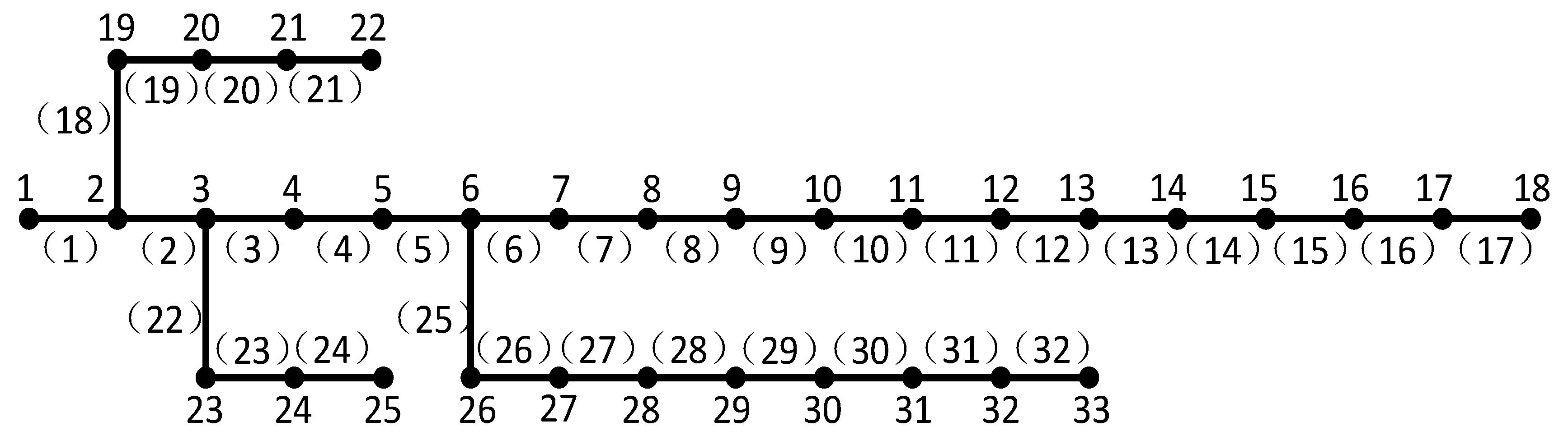
5. Analysis of Example

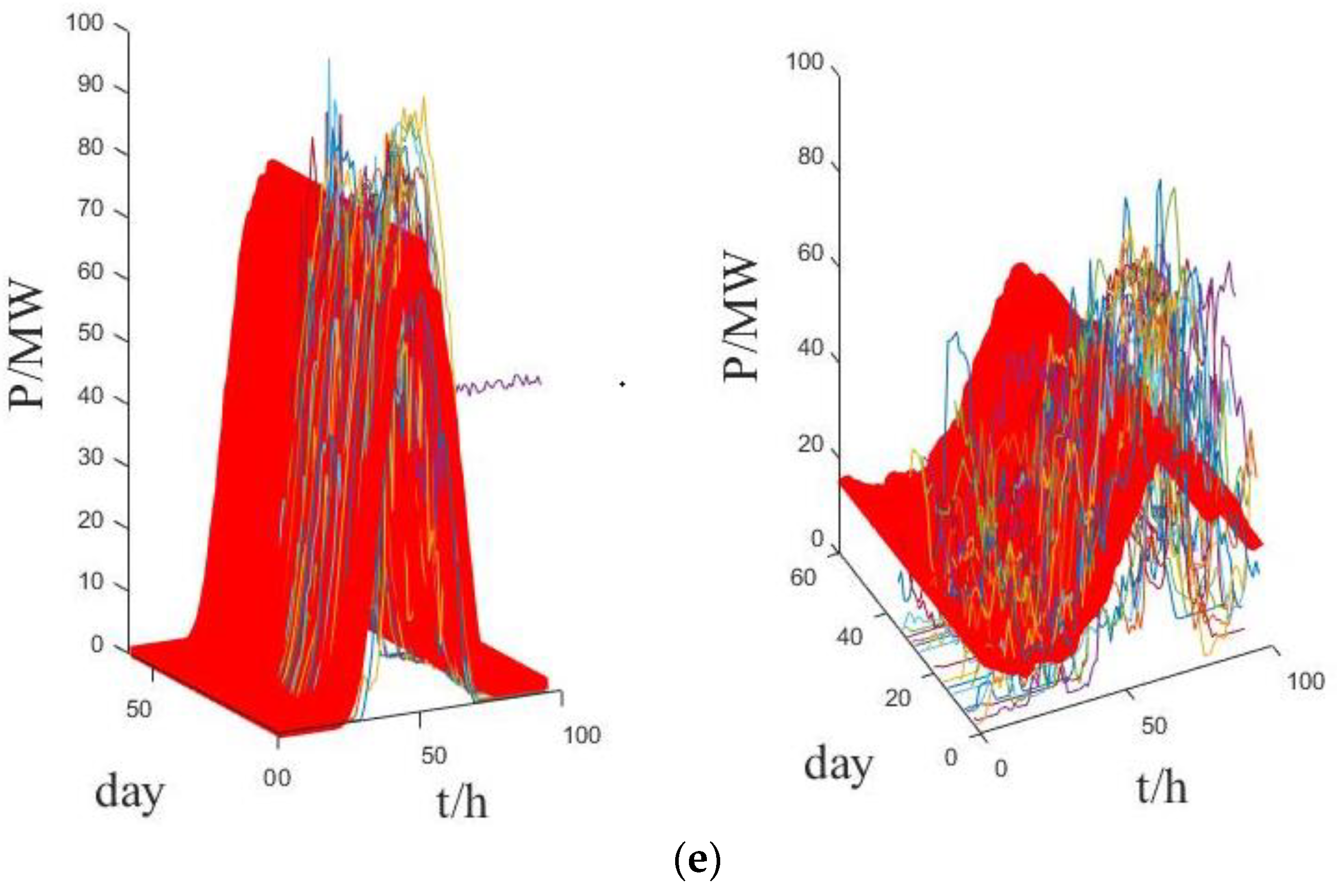
5.1. Basic Data

The IEEE33 radiation system shown in Figure 1 is used to verify the model established in this paper, including voltage reference value U_B = 12.66 kV and power reference value S_B = 100 MVA. The network parameters of the system are detailed in reference [16]. The distribution network includes one wind turbine (WT), one photovoltaic unit (PV), five transferable loads (TL), three interruptible loads (IL) and two energy storage systems (ESS). The specified voltage (nominal value) cannot be lower than 0.95 or higher than 1.05; The upper limit of branch current is 20 kA; The maximum active power and reactive power of purchasing power from the superior power grid cannot be higher than 5 MW. The maximum reactive power cannot be higher than 3 Mvar or lower than −1 Mvar. Output power of generator on node 2 cannot be higher than 1 MW; The upper limit of the capacity of the first ESS is set to 3 MVA, the lower limit is set to 0.18 MVA, and the charging and discharging power cannot be higher than 0.4 MW; The upper limit of the capacity of the second ESS is set to 3 MVA, the lower limit is set to 0.1 MVA, and the charging and discharging power cannot be higher than 0.3 MW; The charging efficiency of ESS is set to 0.9, and the discharging efficiency is set to 1. The total number of running periods T is set to 24. The parameter setting of objective function F in Section 2.1 of this paper is shown in

Table 1. Setting of parameters in objective function.

Parameter	Value
C1	0.50
C2	0.20
Cm,loss	0.35
Closs	0.40

. Through SOCP and the cplex solver in Matlab, the operation optimization of this example is solved directly.

Select the daily time series data of WT and PV output every 15 min for 365 days a year in a certain area (see Figure 2) and the total load curve (see Figure 3). The electricity price data of each moment is shown in Figure 4. WT is connected to 17 nodes, PV is connected to 32 nodes, generator is connected to 2 nodes, ESS access nodes are set to 15 and 23, TL access nodes are set to 5, 7, 13, 14 and 20, and IL access nodes are set to 7, 13 and 19.

It can be found from Figure 2a that the wind turbine has the following output characteristics:

(1)

The output changed significantly throughout the year. The smaller the wind speed in summer and autumn, the smaller the output of the fan. When the wind speed is high in spring and winter, the output of the fan is also high;

(2)

The output varies irregularly in a single day, with randomness and volatility.

It can be found from Figure 2b that photovoltaic units have the following output characteristics:

(1)

Photovoltaic output has obvious periodicity, showing a trend of first increasing and then decreasing;

(2)

Randomness, PV volatility is obvious, and the maximum value is uncertain.

5.2. Identify Typical Scenes

Determine the typical scenes according to the method in Section 1, and cluster the randomly selected time scenes into k scenes. SSE curve obtained by elbow rule is shown in the following figure (Figure 5):

It can be found that SSE decreases rapidly within k = 2 to 5, and then becomes stable after k = 5. k = 5 is an inflection point, and this point is the best k. Therefore, the 365 sample curves in this example are divided into the following five scenes, which is shown in the following figure (Figure 6) (the red curve represents the cluster center of each scene):

The average evaluation of every four moments in the graph can get 24-h clustering results. Analyze these five scenarios separately:

Scenario 1: PV output is up to 76 MW, and WT output is small and stable, indicating that this typical day is sunny and windless;

Scenario 2: PV output is very low, the highest is only 20 MW, WT output is higher and the fluctuation range is not big, indicating that this typical day is cloudy and windy;

Scenario 3: PV output is up to 78 MW, and WT output is very high and unstable at noon, indicating that this typical day is sunny and windy;

Scenario 4: PV and WT output are very low, indicating that this typical day is cloudy and windy;

Scenario 5: PV output is high, and WT output is stable around 15 MW, indicating that this typical day belongs to mild and windy weather.

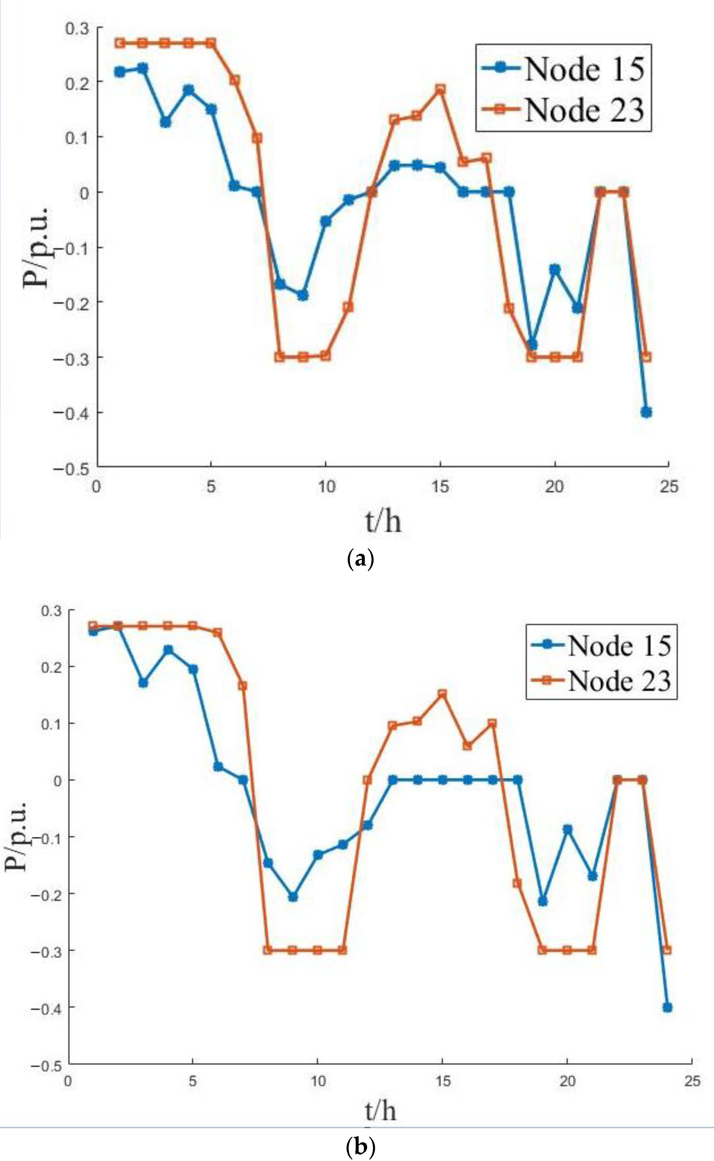
5.3. DNOO Results in Various Clustering Scenes

The optimization results include ESS output, TL output, WT output, PV output, generator output and voltage devision results.

5.3.1. ESS Output Results

The ESS output after operation optimization in five scenes is shown in the following figure (Figure 7):

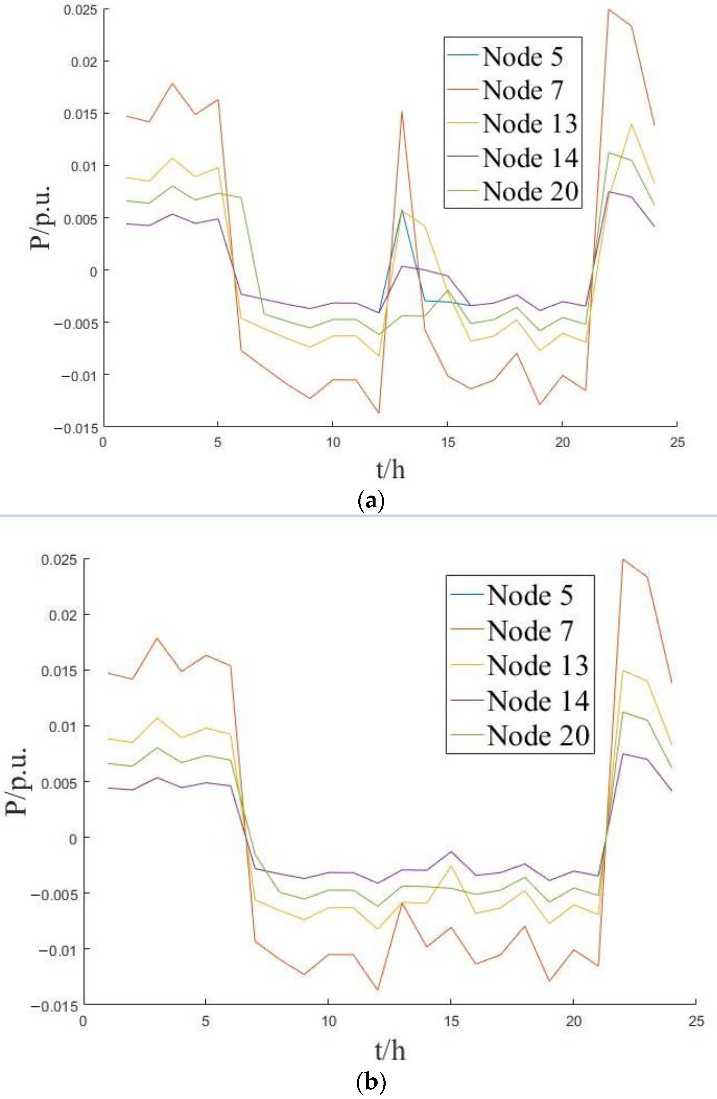
5.3.2. TL Output Results

The TL output after operation optimization in five scenes is shown in the following figure (Figure 8):

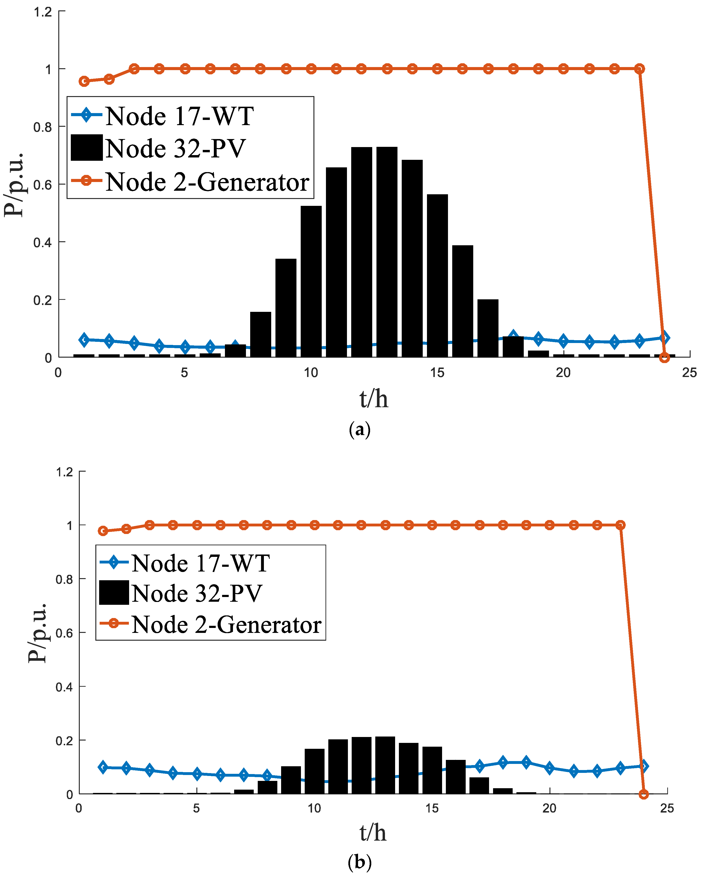
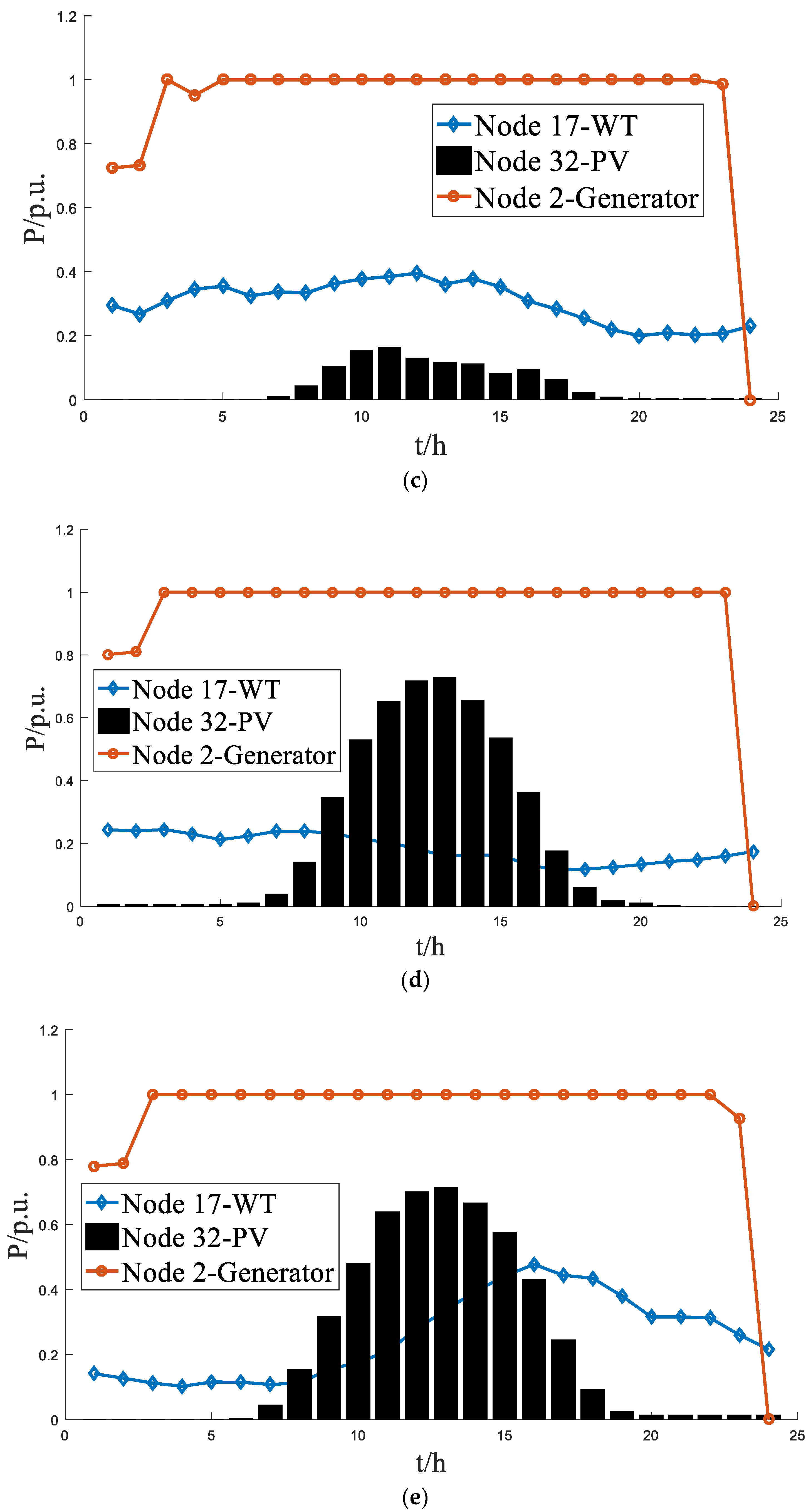
5.3.3. WT, PV and Generator Output Results

The WT, PV, generator output after operation optimization in five scenes is shown in the following figure (Figure 9):

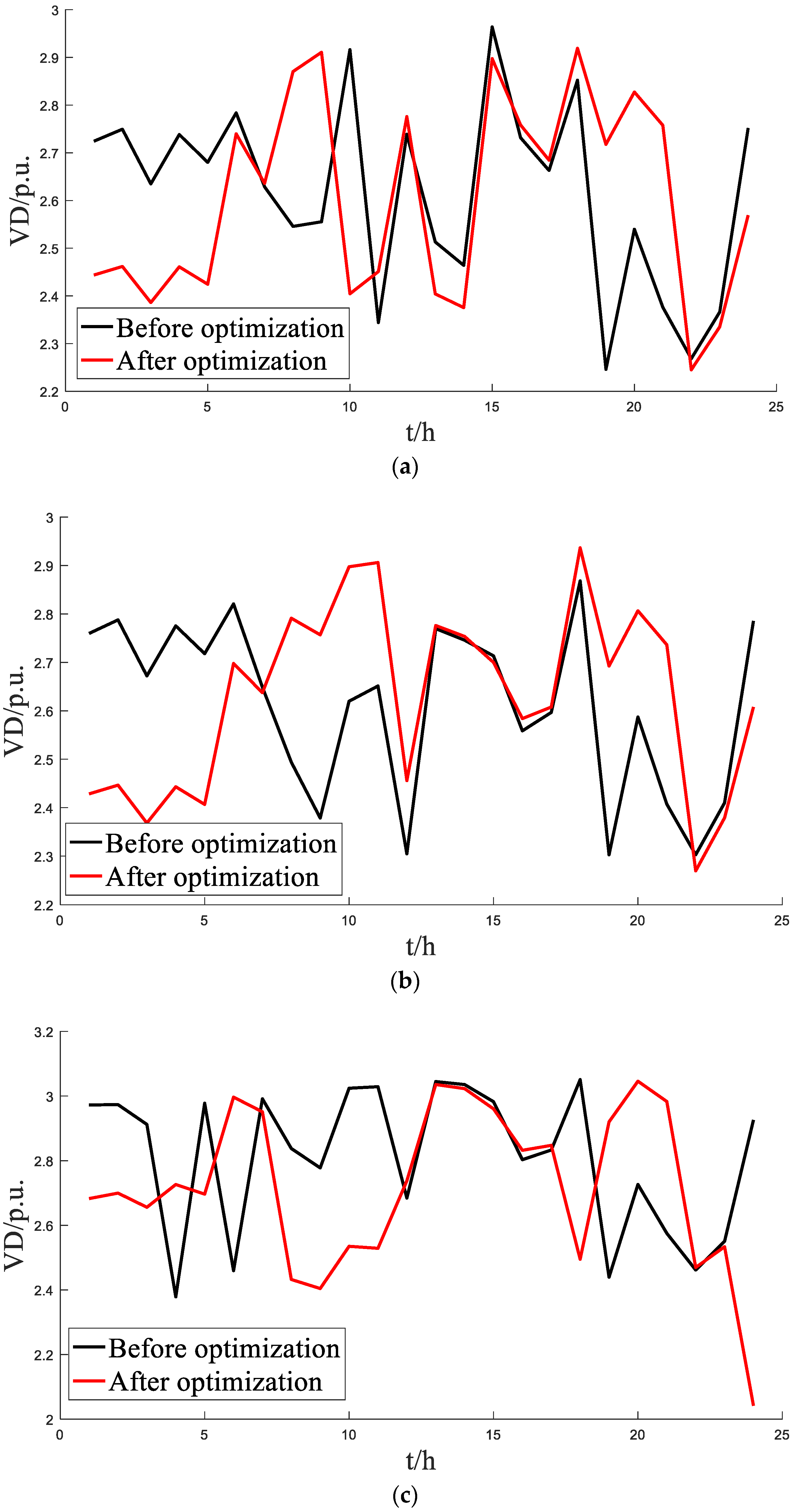
5.3.4. Voltage Deviation (VD) Results

The VD results after operation optimization in five scenes are shown in the following figure (Figure 10):

Analyze with reference to Figure 7, Figure 8, Figure 9 and Figure 10 and

Table 2. Cost Analysis of Different Scenes.

Scene Sequence Number		Cm (Yuan)	CDR (Yuan)	CESS.loss (Yuan)	CEP (Yuan)	Cpl (Yuan)	Total Cost (Yuan)	Total VD (p.u.)
1	Before	2218.96	0.00	0.00	9170.20	3495.70	20,085.00	62.78
	After	8022.57	276.04	197.86	6735.84	3512.83	18,745.13	54.54
2	Before	1216.88	0.00	0.00	11,178.00	3751.10	22,280.00	62.68
	After	8036.60	279.87	206.42	8583.81	3768.74	20,875.43	55.17
3	Before	2948.64	0.00	0.00	8733.30	2810.70	18,417.00	67.45
	After	7838.63	262.90	206.64	5928.41	2852.37	17,088.96	57.31
4	Before	3311.53	0.00	0.00	7802.70	2719.50	17,544.00	64.60
	After	7913.94	260.79	189.39	5104.19	2718.05	16,186.36	56.46
5	Before	3936.21	0.00	0.00	6758.60	2566.20	16,304.00	64.76
	After	7873.91	224.72	182.68	4152.56	2575.14	15,009.01	55.90

:

Scene 1: The two ESS are in a charging state most of the time; The output of TL connected to node 7 varies greatly from 12 00 to 15:00; The output of the generator reaches the upper limit at 3:00~23:00; The total operating cost is reduced by 6.67% compared with that before optimization, and the total voltage deviation at 24 h is reduced by 13.13% during optimization;

Scene 2: The ESS connected to the 3-node reaches the upper limit of charging power at 8:00~11:00 and 19:00~21:00; TL output is stable from 8:00 to 21:00; The output of the generator reaches the upper limit from 3: 00 to 23: 00; The total operating cost is reduced by 6.30% compared with that before optimization, and the total voltage deviation at 24 h is reduced by 11.98% during optimization;

Scene 3: During the periods of 1:00~7:00 and 12:00~17:00, the discharge of ESS connected to the 23-node is more than that of ESS connected to the 15-node, and the output reaches the upper limit of charging power at 8:00~11:00 and 19:00~21:00. Except the TL connected to nodes 13 and 14, the output of other TL is stable from 8: 00 to 21:00; The output of the generator reaches the upper limit from 5:00 to 22:00; The total operating cost is reduced by 7.21% compared with that before optimization, and the total voltage deviation at 24 h is reduced by 15.03% during optimization;

Scene 4: From 1:00 to 18:00, the output of ESS connected with 23 nodes is more than that connected with 15 nodes, whether charging or discharging; Only the output of TL connected to node 20 is stable from 8:00 to 21:00; The output of the generator reaches the upper limit from 3:00 to 23:00; The total operating cost is reduced by 7.74% compared with that before optimization, and the total voltage deviation at 24 h is reduced by 12.6% during optimization;

Scene 5: From 14:00 to 18:00, the ESS connected to node 15 discharged more; Only the TL output of node 20 is stable from 8: 00 to 21: 00; The output of the generator reaches the upper limit from 3:00 to 22:00; The total operating cost is reduced by 7.94% compared with that before optimization, and the total voltage deviation at 24 h is reduced by 13.68% during optimization.

6. Conclusions

Research on the operation optimization method of distribution network with wind and solar power units plays a vital role in the management and operation of the whole power system, and can improve the security and stability of the system. In this paper, the DNOO model is established, and the second-order cone method is used to solve the model. The effectiveness of this method is verified based on IEEE33-bus system. The conclusions are as follows:

(1)

Cluster and divide the WT and PV output of 365 days a year, and cluster them into typical scenes, so as to obtain the scenery cluster center of each scene, which can basically cover the annual operation characteristics of the distribution system during the subsequent optimization;

(2)

When the DNOO model is established, the load storage of the source network is considered comprehensively, the lowest total operating cost including unit operating cost, demand response cost and network loss cost is taken as the objective function, and the conditions such as power flow constraint, demand response constraint and energy storage device constraint are considered comprehensively. It is more in line with the actual distribution network operation, and the index improvement degree is obvious;

(3)

The results obtained by the second-order cone method and the Cplex solver show that the calculation results of this method can obtain the lowest total operating cost of each typical scenario on the basis of the total absorption of wind and light, thus ensuring the efficient operation of the power grid system.

References

1. Zailin, P.; Xiaofang, M. Distribution Network Planning; Electric Power Press: Beijing, China, 2015; pp. 180–197. [Google Scholar]
2. Kaiyan, W.; Haodong, D.; Rong, J.; Heng, L.; Yan, L.; Xueyan, W. Short-term Interval Probability Prediction of Photovoltaic Power Based on Similar Daily Clustering and QR-CNN-BiLSTM Model. High Volt. Eng. 2022, 48, 4372–4388. [Google Scholar]
3. Zhifeng, H.; Jing, C.; Jingfei, Z.; Chunke, L.; Qian, B.; Ke, C. Optimal Dispatch of Active Distribution Network Considering Uncertainty Boundary of Renewable Power Generation. Smart Power 2022, 50, 48–55. [Google Scholar]
4. Mehbodniya, A.; Paeizi, A.; Rezaie, M.; Azimian, M.; Masrur, H.; Senjyu, T. Active and Reactive Power Management in the Smart Distribution Network Enriched with Wind Turbines and Photovoltaic Systems. Sustainability 2022, 14, 4273. [Google Scholar] [CrossRef]
5. Mingqiang, X.; Jun, L.; Shuqing, W.; Ning, Y.; Hong, H. Damage detection of wind turbine blades by Bayesian multivariate cointegration. Ocean Eng. 2022, 258, 111603. [Google Scholar]
6. Jinsheng, C.; Jun, Z.; Junfeng, L.; Feng, X. Distributionally Robust Optimization Method for Grid-connected Microgrid Considering Extreme Scenarios. Autom. Electr. Power Syst. 2022, 46, 50–59. [Google Scholar]
7. Shan, C.; Mengyu, Z.; Kaixuan, N.; Zhaobin, W. Design Optimization of Microgrid Based on Generalized Demand Side Resources. Mod. Electr. Power 2020, 37, 180–186. [Google Scholar]
8. Chunyan, L.; Chenyu, Z.; Bo, H.; Zhengyu, C.; Qinglong, L.; Lingyun, W.; Kaigui, X. Two-stage clustering algorithm of typical wind-PV-load scenario generation for reliability evaluation. Adv. Technol. Electr. Eng. Energy 2021, 40, 1–9. [Google Scholar]
9. Jiayi, W.; Hongjun, G.; Youbo, L.; Junyong, L.; Xiaodong, Y.; Shuaijia, H. A Distributed Operation Optimization Model for AC/DC Hybrid Distribution Network Considering Wind Power Uncertainty. Proc. CSEE 2020, 40, 550–563. [Google Scholar]
10. Tao, Z.; Ran, H.; Jing, L.; Yihong, L.; Liming, H. Multi-objective Optimal Operation of Distribution Network With High Penetration of New Energy Based on Flexible Interconnection Technology. Smart Power 2021, 49, 1–7+55. [Google Scholar]
11. Bo, Z.; Junzhi, R.; Jian, C.; Da, L.; Ruwen, Q. Tri-level robust planning-operation co-optimization of distributed energy storage in distribution networks with high PV penetration. Appl. Energy 2020, 279, 115768. [Google Scholar]
12. Sijie, C.; Yongbiao, Y.; Minglei, Q.; Qingshan, X. Coordinated multiobjective optimization of the integrated energy distribution system considering network reconfiguration and the impact of price fluctuation in the gas market. Int. J. Electr. Power Energy Syst. 2022, 138, 107776. [Google Scholar]
13. Haiguo, T.; Zhidan, Z.; Tong, K.; Di, Z.; Cong, Z.; Bo, L. Bi-level Stochastic Operation Optimization of Distribution- Natural Gas Combined System Considering Scenario Clustering. Mod. Electr. Power 2021, 38, 681–694. [Google Scholar]
14. Bin, W.; Xiaoqing, H.; Wen, L.; Lingjuan, G.; Hao, Y. Multi-time Scale Stochastic Optimal Dispatch for AC/DC Hybrid Microgrid Incorporating Multi-scenario Analysis. High Volt. Eng. 2020, 46, 2359–2369. [Google Scholar]
15. Yanfeng, M.; Yu, F.; Shuqiang, Z.; Xiaokuan, Y.; Zijian, W.; Ling, D.; Fanfei, Z. Capacity allocation of new energy source based on wind and solar resource scenario simulation using WGAN and sequential production simulation. Electr. Power Autom. Equip. 2020, 40, 77–86. [Google Scholar]
16. Yanfeng, M.; Jiarong, X.; Shuqiang, Z.; Zijian, L.; Zerong, L. Multi-objective Optimal Dispatching for Active Distribution Network Considering Park-level Integrated Energy System. Autom. Electr. Power Syst. 2022, 46, 53–61. [Google Scholar]
17. Buxiang, Z.; Yibin, X. Optimal Scheduling of Source-load Interactive Micro-grid Based on Machine Learning. Proc. CSU-EPSA 2022, 34, 144–150. [Google Scholar]
18. Ruxiang, M.; Kangning, Y.; Lin, S.; Ke, X.; Dechun, Z. Operational flexibility evaluation of distribution network considering scenario clustering. Power DSM 2021, 23, 86–91. [Google Scholar]
19. Kun, H.; Zhihan, L.; Ming, F.; Xiaobo, D.; Xiaoyan, Z. Optimal Dispatch of AC/DC Distribution Network Considering Voltage Risk Perception. Autom. Electr. Power Syst. 2021, 45, 45–54. [Google Scholar]
20. Ran, Q.; Guobin, J.; Qing, X.; Guoqing, L.; Di, P.; Chao, S. Optimal Dispatching of DC Distribution Network Based on Source-grid-load-storage Interactions. Proc. CSU-EPSA 2021, 33, 41–50. [Google Scholar]
21. Shan, C.; Ziming, C.; Rui, W.; Lijun, H.; Zhaobin, W. Double -layer coordinated optimal dispatching of multi -microgrid based on mixed game. Electr. Power Autom. Equip. 2021, 41, 41–46. [Google Scholar]
22. Shibo, Y.; Liang, S.; Lidong, C.; Jiayu, C. Coordinated optimal scheduling of distribution network with CCHP-based microgird considering time-of-use electricity price. Electr. Power Autom. Equip. 2021, 41, 15–23. [Google Scholar]
23. Nan, N.; Lin, D.; Xingyan, L.; Lu, Y.; Youbo, L. Robust Optimal Power Flow of Active Distribution Network Based on Imprecise Dirichlet Model. Proc. CSU-EPSA 2021, 33, 20–28. [Google Scholar]
24. Ruijie, C.; Zongxiang, L.; Ying, Q. Optimal Dispatch Based on Multi-scene Ambiguity Set and Modified Second-order Cone Algorithm for Distribution Network. Power Syst. Technol. 2021, 45, 4621–4629. [Google Scholar]
25. Mubarak, H.; Muhammad, M.A.; Mansor, N.N.; Mokhlis, H.; Ahmad, S.; Ahmed, T.; Sufyan, M. Operational Cost Minimization of Electrical Distribution Network during Switching for Sustainable Operation. Sustainability 2022, 14, 4196. [Google Scholar] [CrossRef]
26. Olorunfemi, T.R.; Nwulu, N.I. Multi-Agent Based Optimal Operation of Hybrid Energy Sources Coupled with Demand Response Programs. Sustainability 2021, 13, 7756. [Google Scholar] [CrossRef]
27. Yao, X.; Zhaohong, B.; Gechao, H.; Gengfeng, L.; Xiaosong, G.; Shiyu, L.; Yuankang, H.; Ruifeng, L. Chance-constrained Distributional Robust Optimization Based on Second-order Cone Optimal Power Flow. Power Syst. Technol. 2021, 45, 1505–1518. [Google Scholar]
28. Yuqin, X.; Nan, F. Multi Objective Optimal Scheduling of Electricity-Gas Interconnected System Based on Piecewise Linearization and Improved Second-Order Cone Relaxation. Trans. China Electrotech. Soc. 2022, 37, 2800–2812. [Google Scholar]
Figure 1. IEEE33-node radial distribution network.
Sustainability 15 02184 g001
Figure 2. Timing diagram of wind and solar power generation day: (a) WT; (b) PV.
Sustainability 15 02184 g002aSustainability 15 02184 g002b
Figure 3. Total load curve.
Sustainability 15 02184 g003
Figure 4. Electricity purchase price.
Sustainability 15 02184 g004
Figure 5. Intra-cluster error variance curve.
Sustainability 15 02184 g005
Figure 6. Photovoltaic and wind power curves in typical scenes: (a) Scene 1; (b) Scene 2; (c) Scene 3; (d) Scene 4; € Scene 5.
Sustainability 15 02184 g006aSustainability 15 02184 g006bSustainability 15 02184 g006c
Figure 7. ESS: (a) Scene 1; (b) Scene 2; (c) Scene 3; (d) Scene 4; (e) Scene 5.
Sustainability 15 02184 g007aSustainability 15 02184 g007b
Figure 8. TL: (a) Scene 1; (b) Scene 2; (c) Scene 3; (d) Scene 4; (e) Scene 5.
Sustainability 15 02184 g008aSustainability 15 02184 g008b
Figure 9. WT, PV, generator: (a) Scene 1; (b) Scene 2; (c) Scene 3; (d) Scene 4; (e) Scene 5.
Sustainability 15 02184 g009aSustainability 15 02184 g009b
Figure 10. Voltage deviation: (a) Scene 1; (b) Scene 2; (c) Scene 3; (d) Scene 4; (e) Scene 5.
Sustainability 15 02184 g010aSustainability 15 02184 g010b