
Traffic Circle—An Example of Sustainable Home Zone Design

Abstract
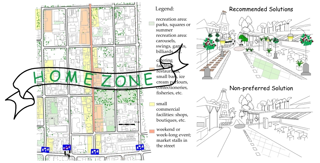
:
1. Introduction
- −
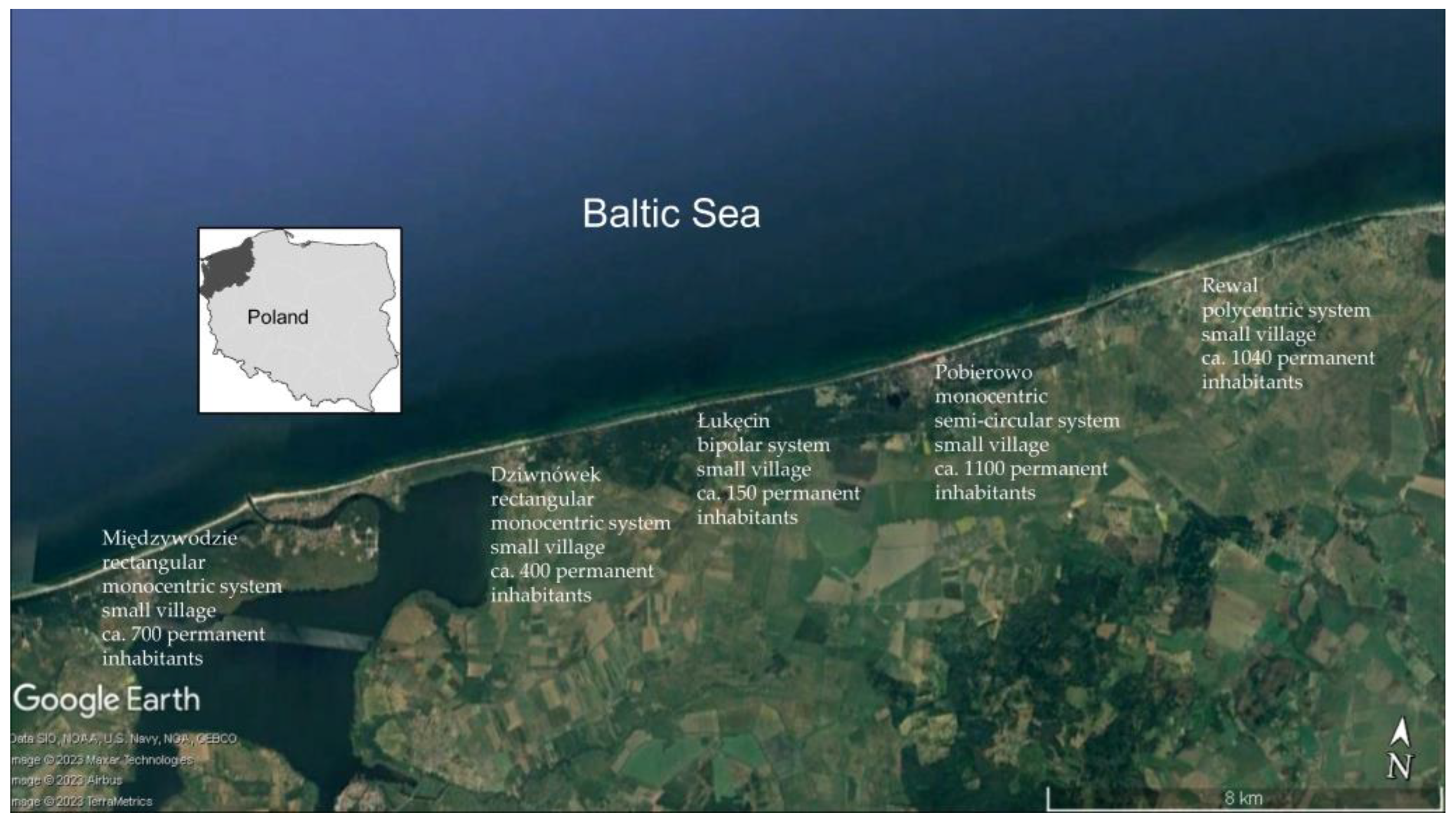
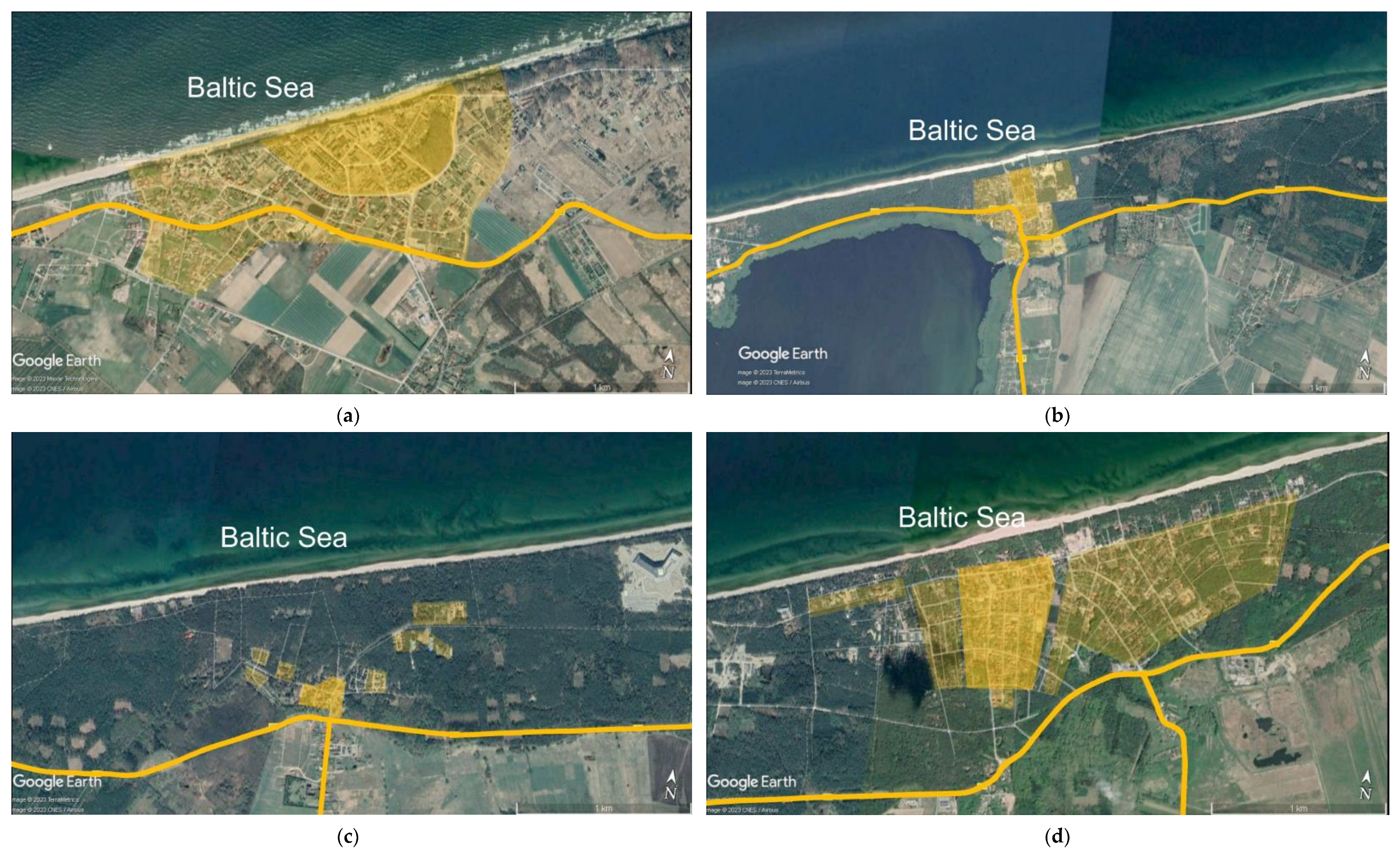
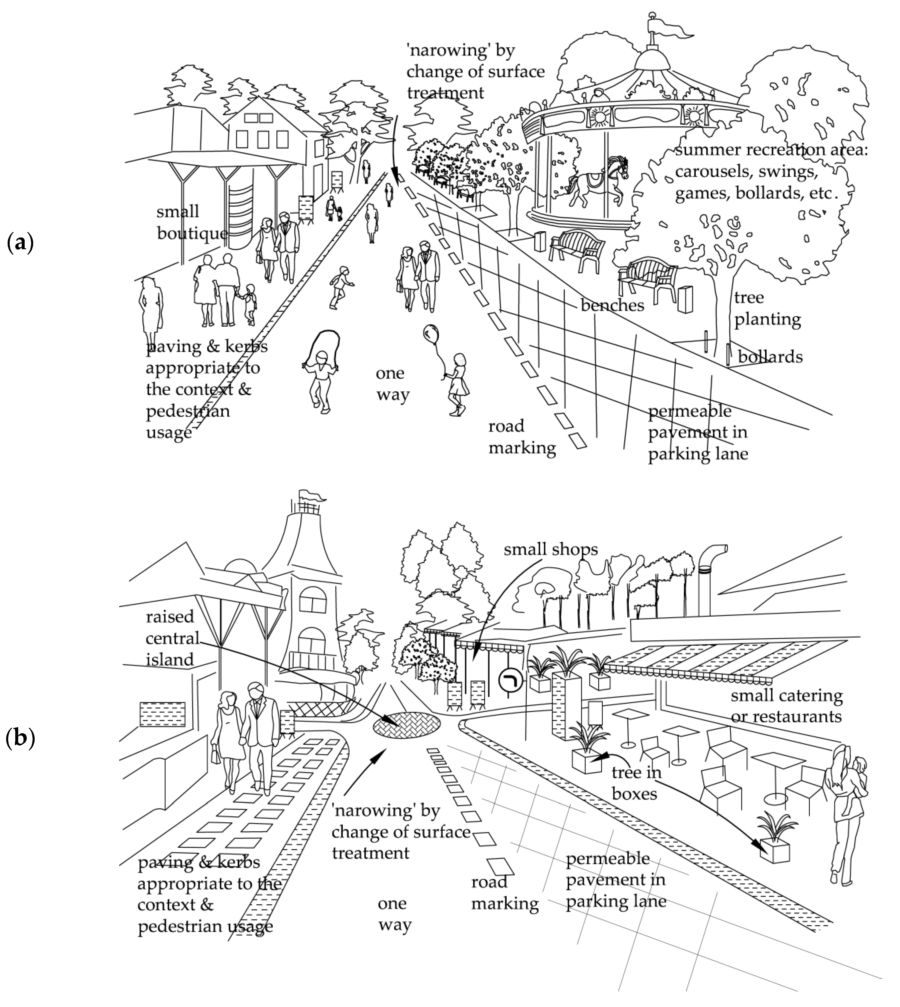
- monocentric, with a clear-cut centre both functionally and spatially and a generally oblong, elliptical, square, rectangular or semi-circular shape (Figure 2a,b),
- −
- bipolar, made up of two or more distinctly bordered urban entities that may merge into a rectangular or tubular system (Figure 2c),
- −
- polycentric, formed through development and merging of smaller entities (Figure 2d).
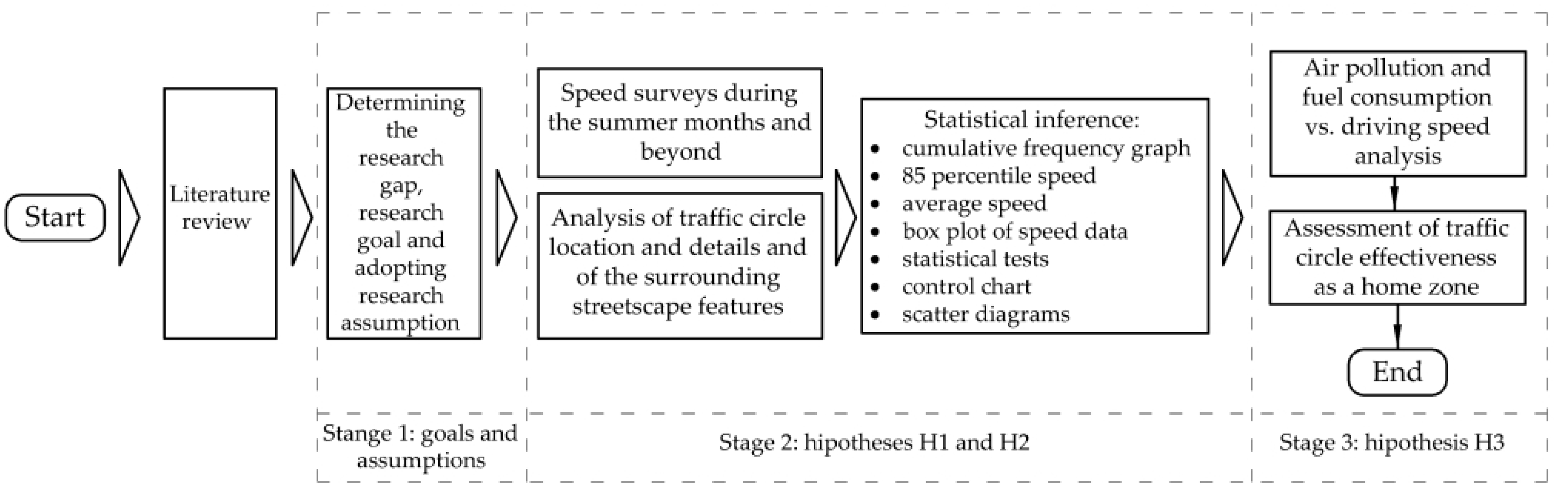
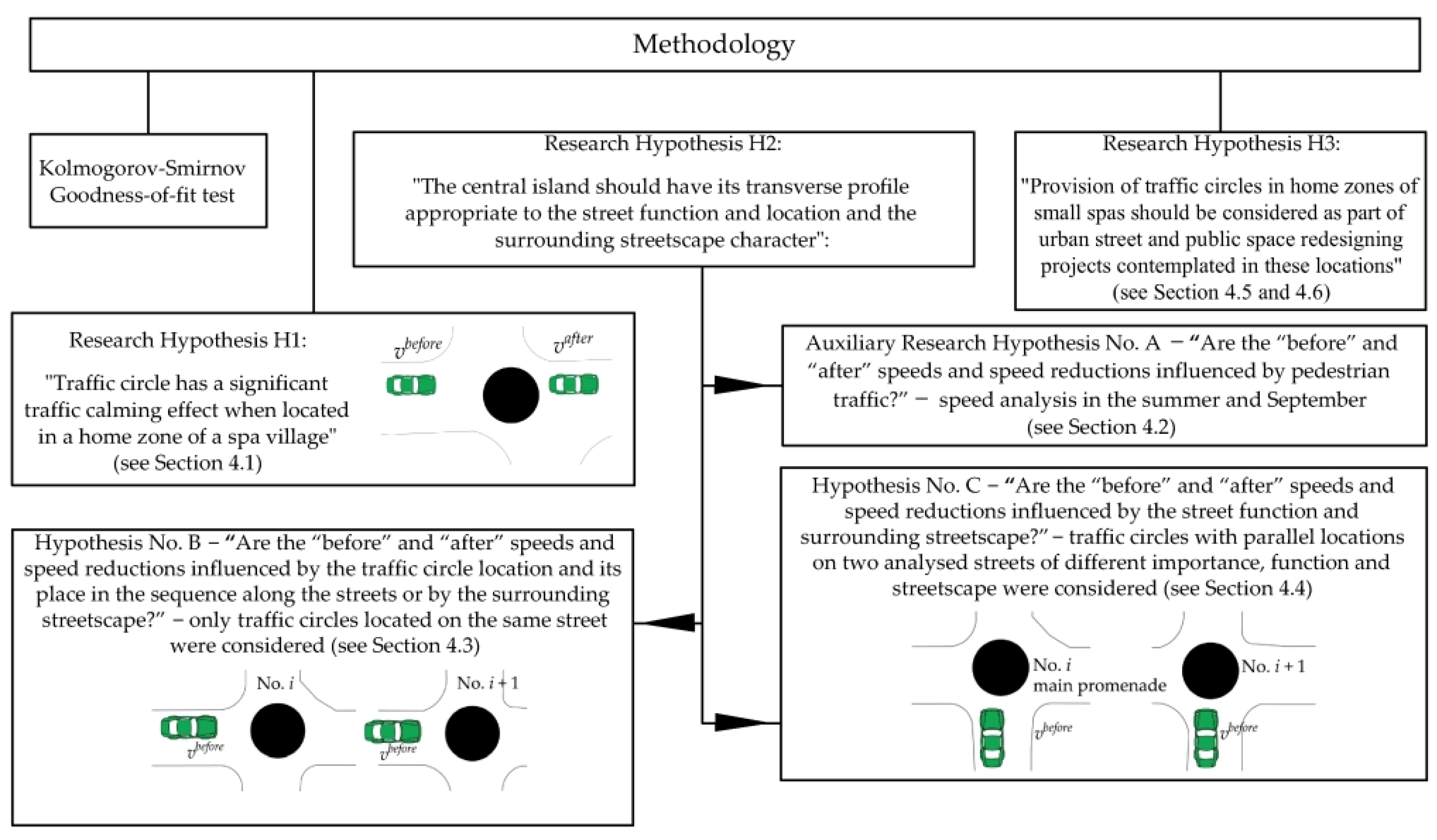
2. Materials and Methodology
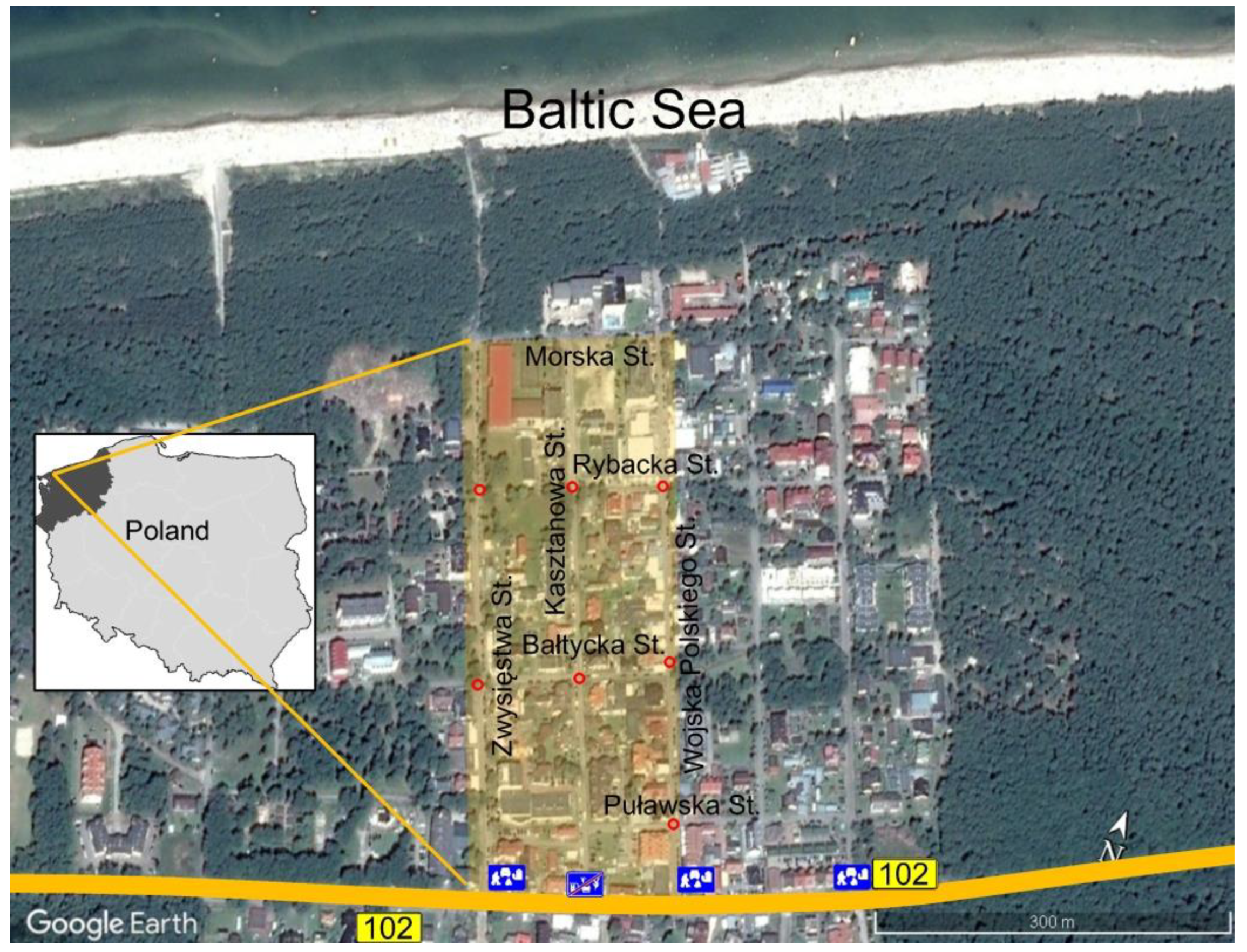
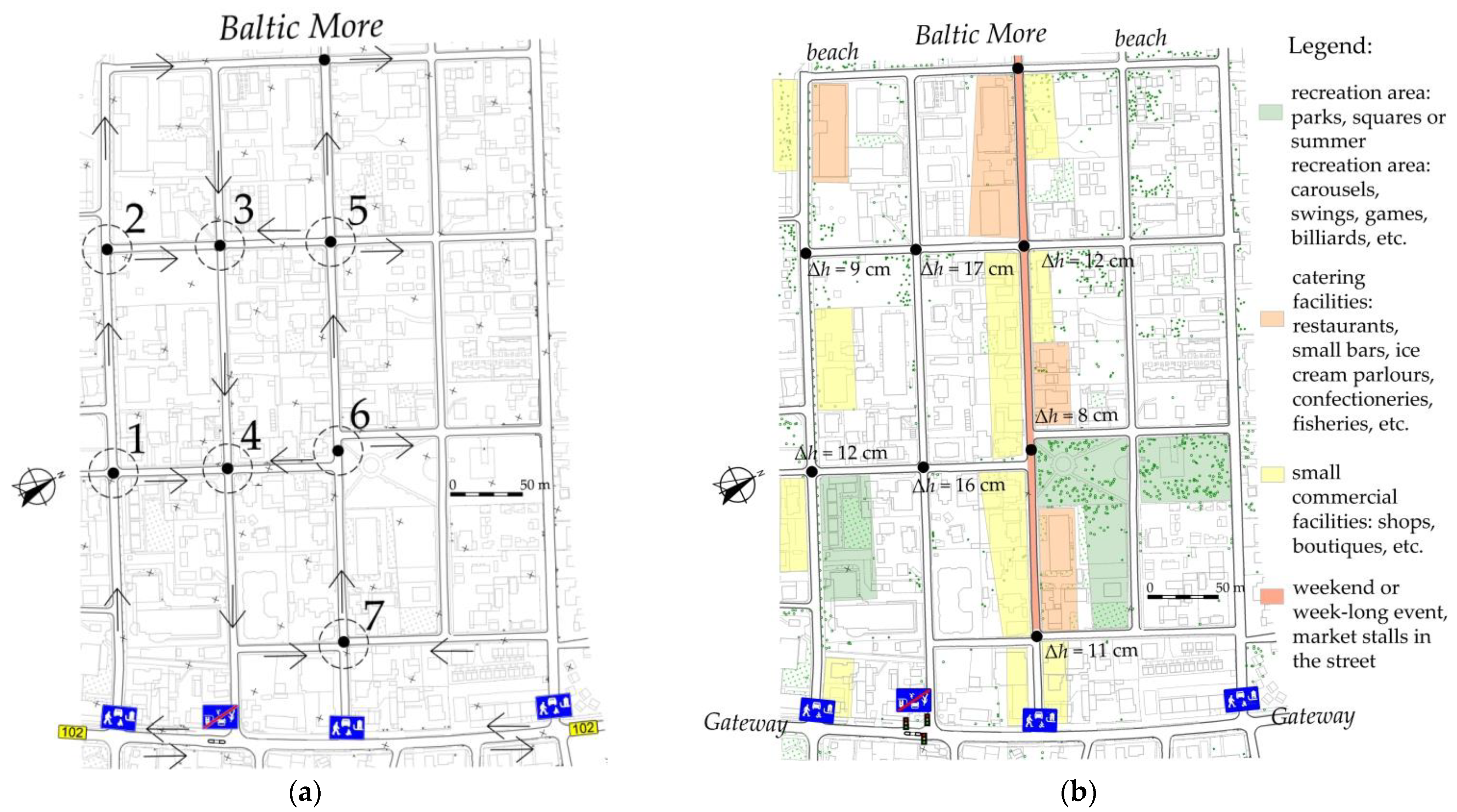
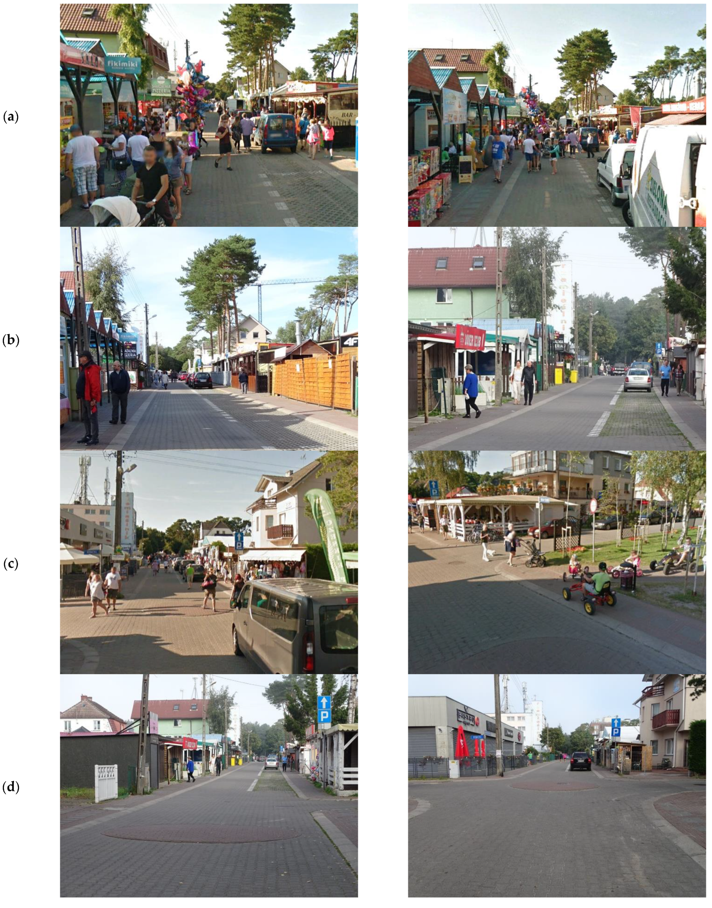
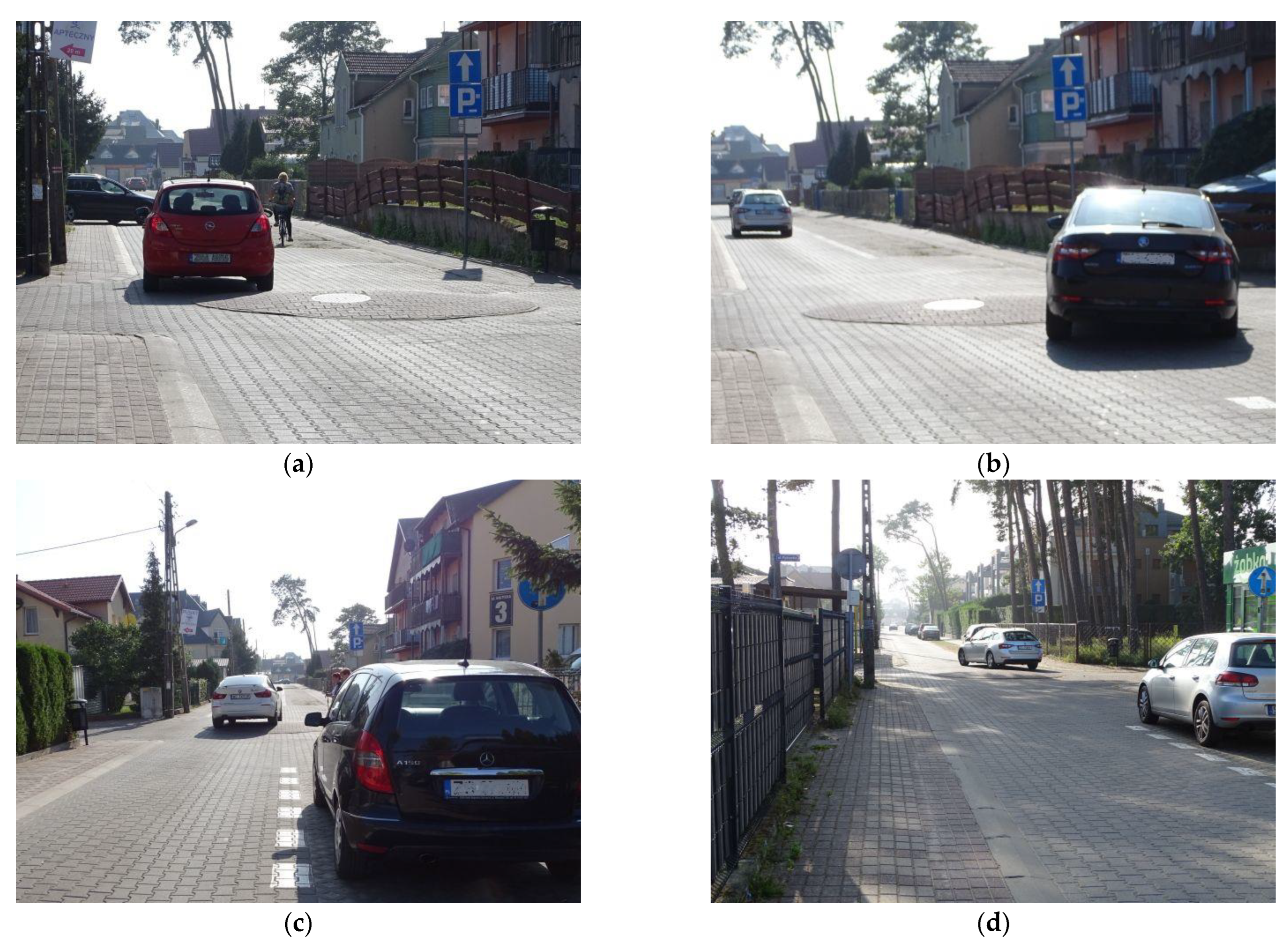
2.1. Study Area
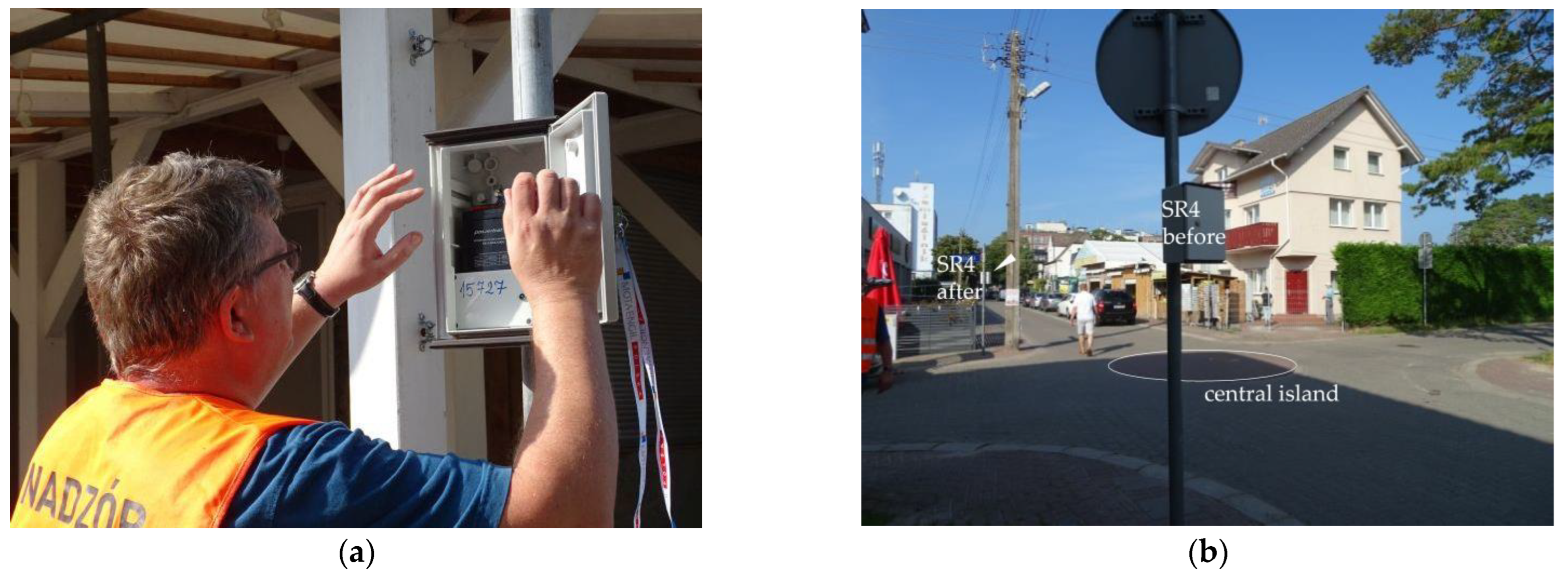
2.2. Traffic Volume and Speed Surveys
2.3. Methodology
3. Results
3.1. Characteristics of the Traffic Calming Measurement TCM
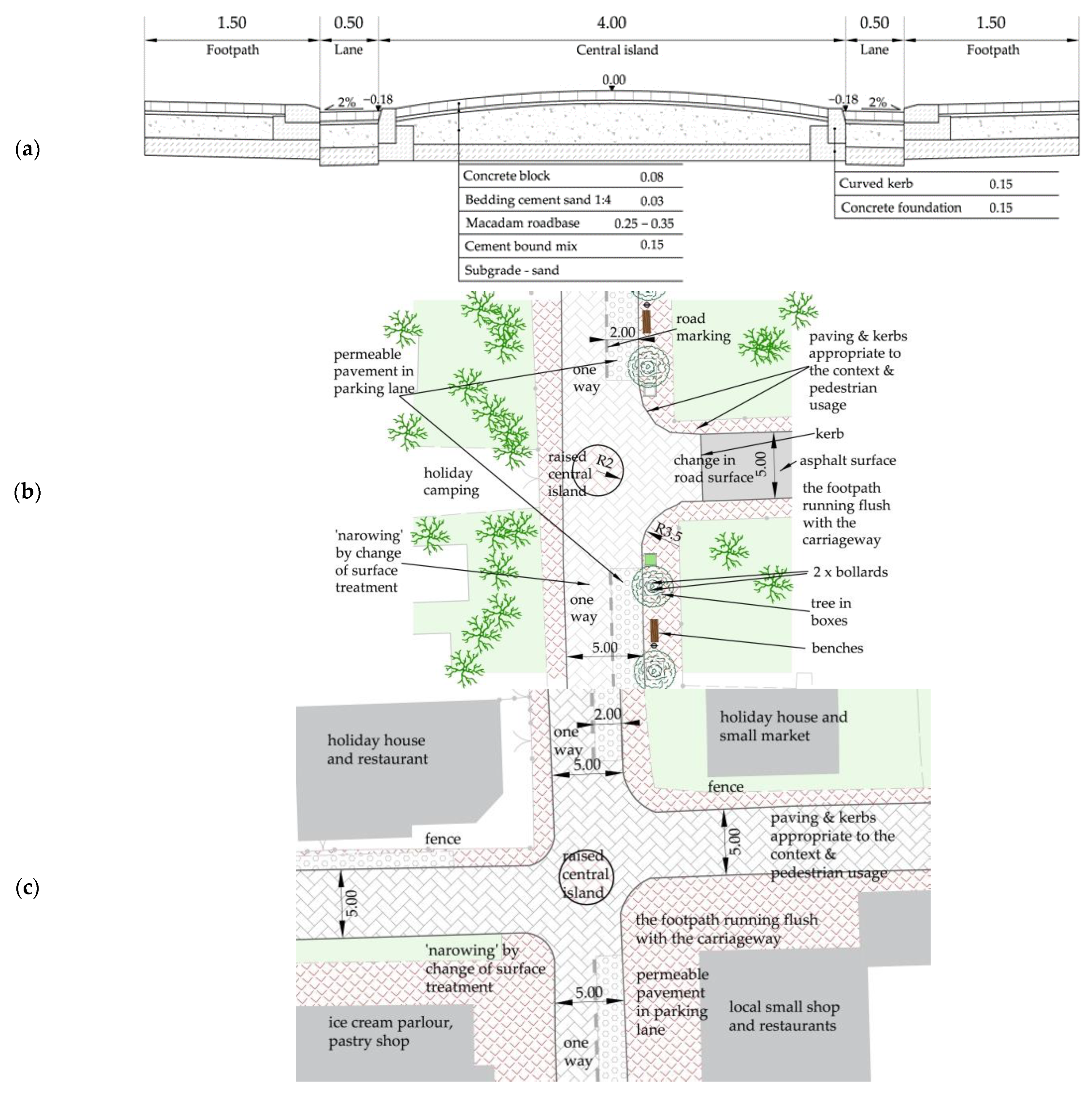
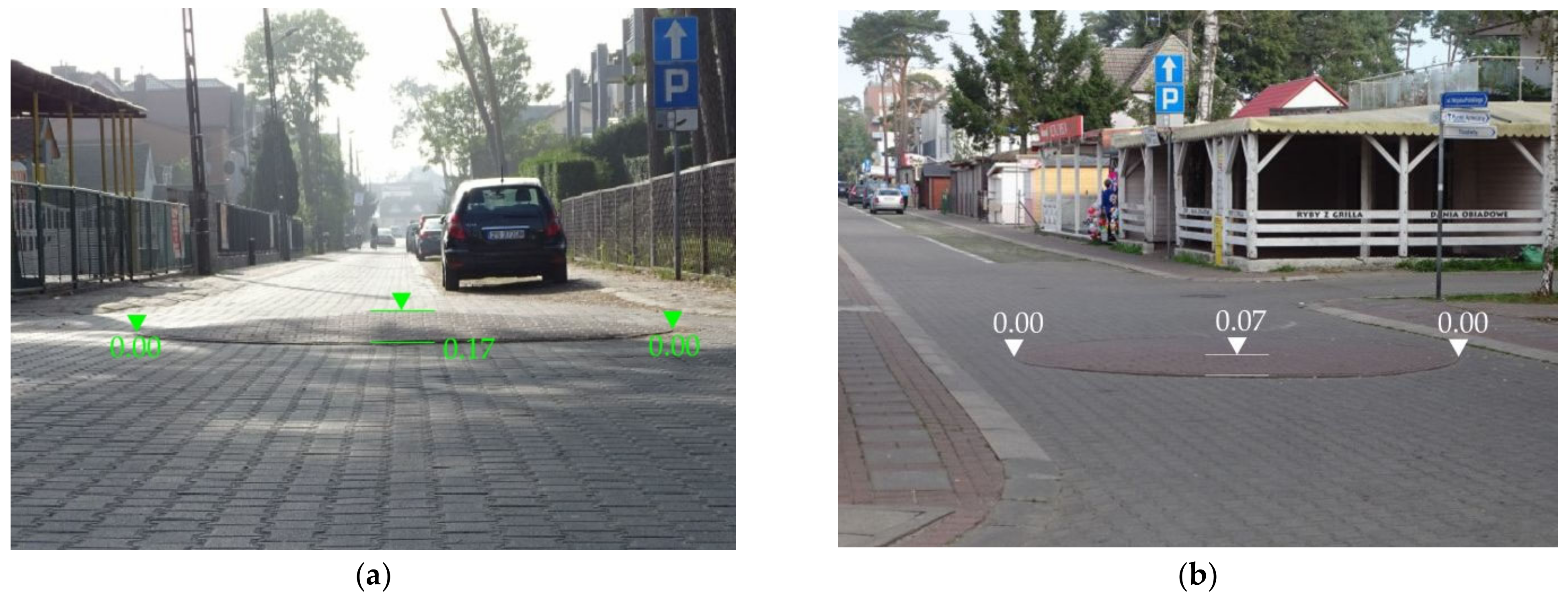
3.2. Plan and Cross-Section of Selected Traffic Circles
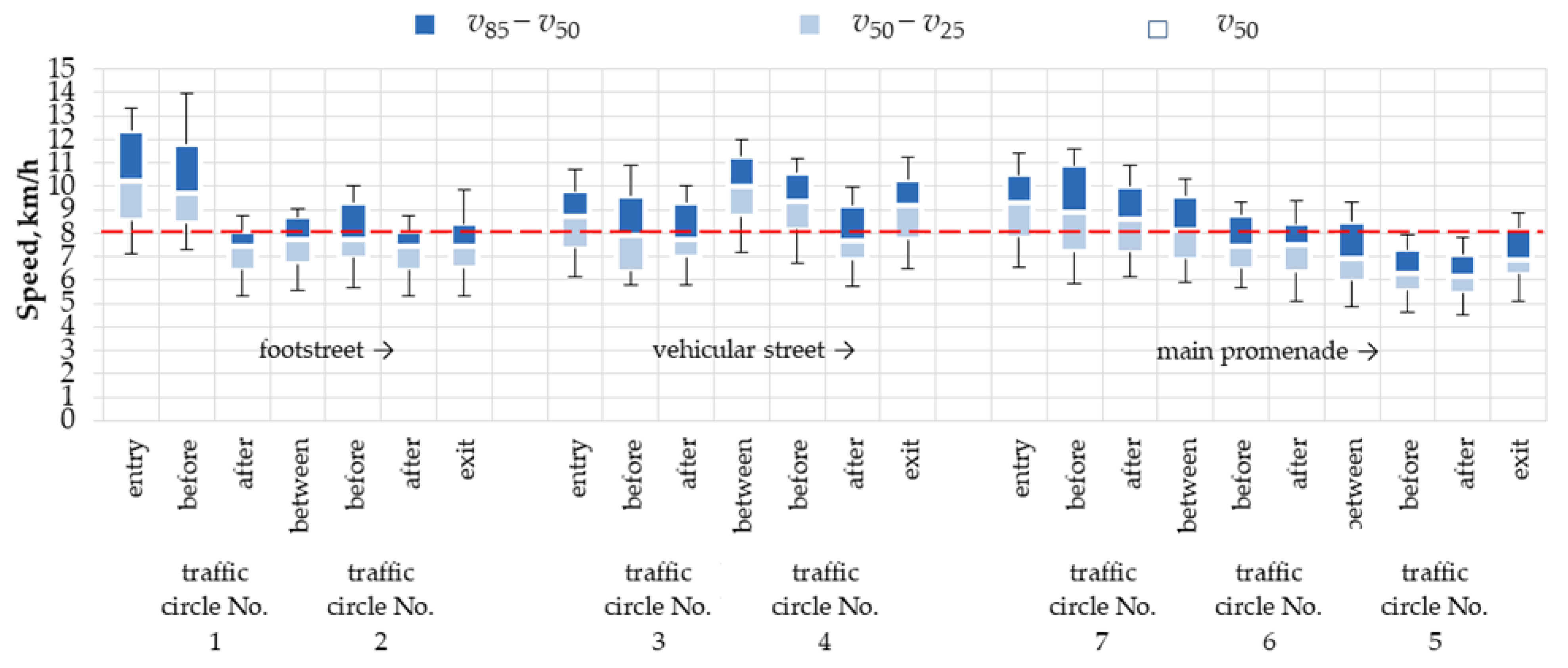
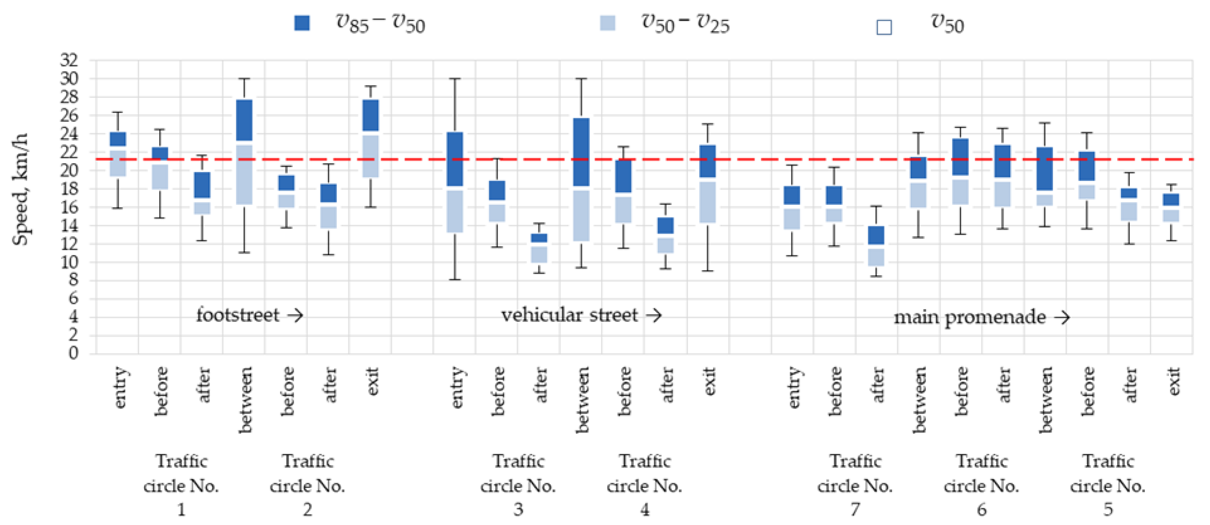
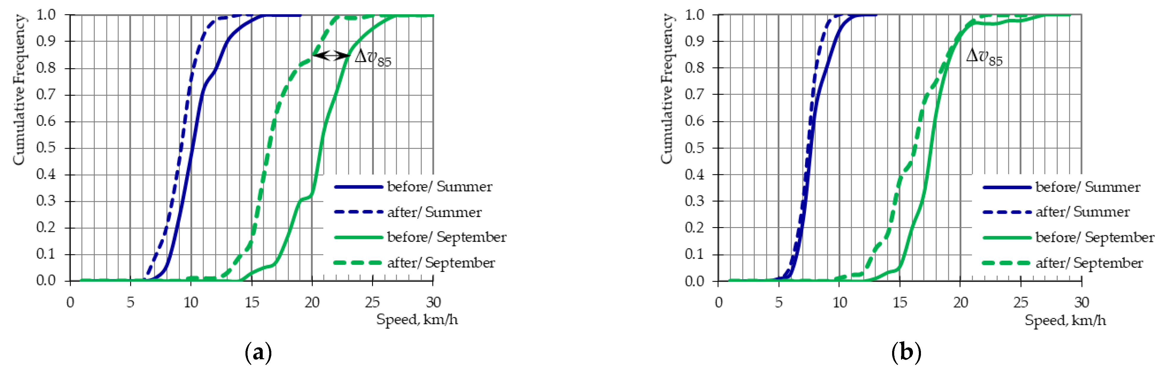
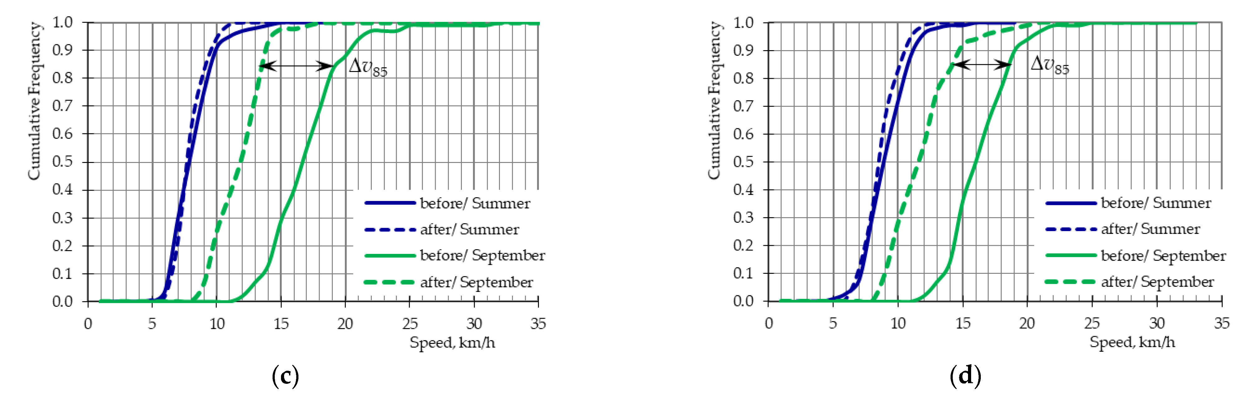
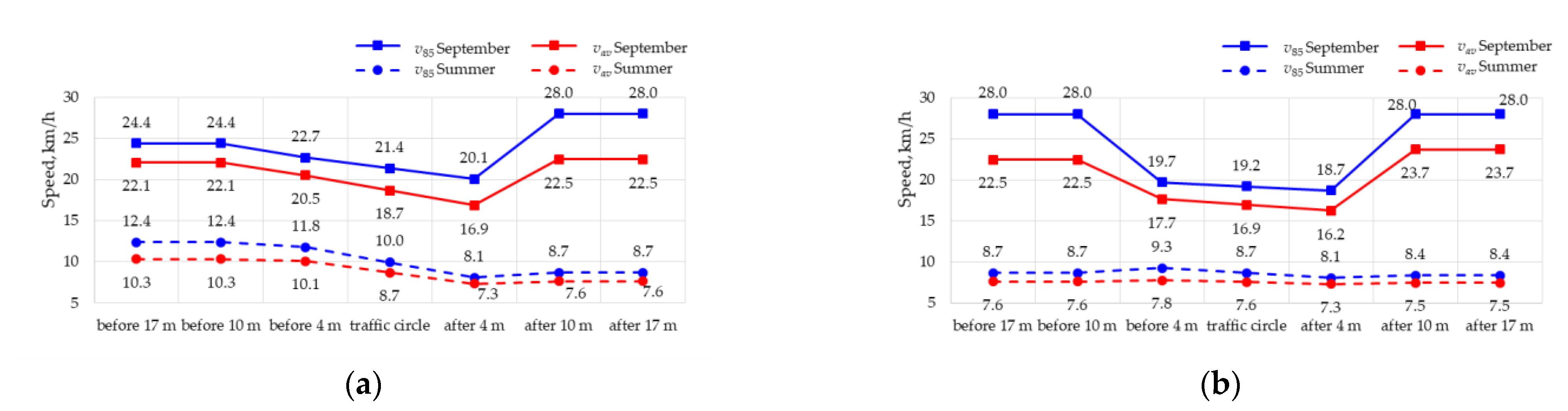
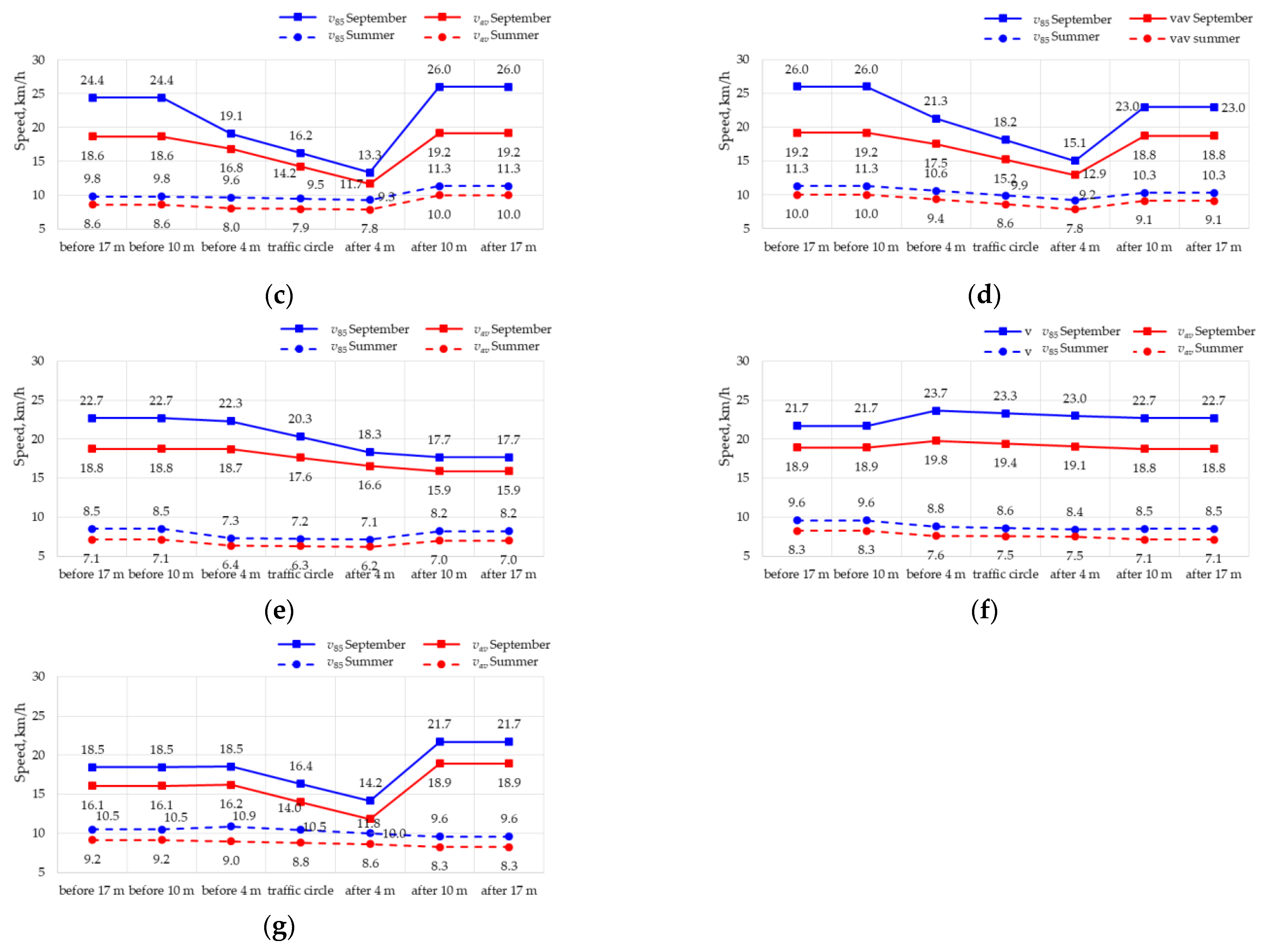
3.3. Speed Survey Data Processing
4. Discussion
4.1. Research Hypothesis H1—“A Traffic Circle Has a Significant Traffic Calming Effect When Located in a Home Zone of a Spa Village”
4.2. Research Hypothesis H2—“The Central Island Should Have Its Transverse Profile Appropriate to the Street Function and Location and the Surrounding Streetscape Character”
4.2.1. Auxiliary Hypothesis 2A—“Are the “Before” and “After” Speeds and Speed Reductions Influenced by Pedestrian Traffic?”
4.2.2. Auxiliary Hypothesis 2B—“Are the “Before” and “After” Speeds and Speed Reductions Influenced by the Traffic Circle Location and Its Place in the Sequence along the Streets or by the Surrounding Streetscape?”
4.2.3. Auxiliary Hypothesis 2C—“Are the “before” and “after” Speeds and Speed Reductions Influenced by the Street Function and Surrounding Streetscape?”
4.3. Trajectory and Speed Profile Analysis
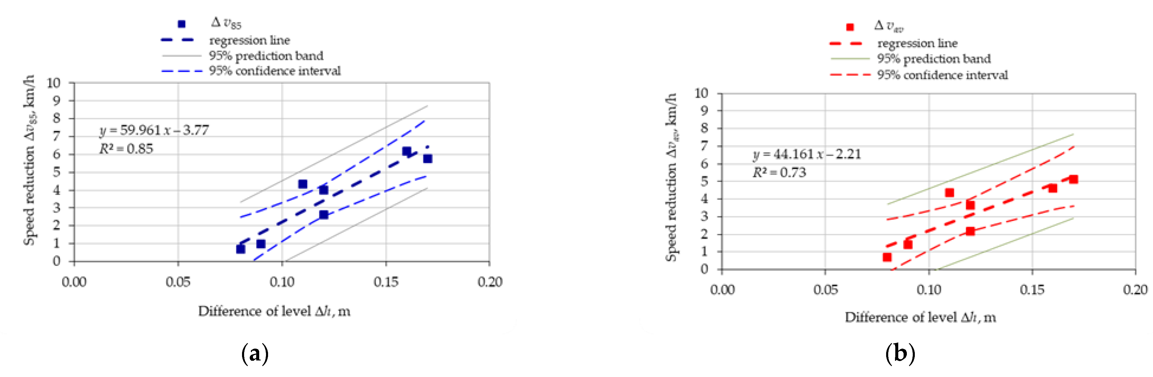
4.4. Regression Analysis
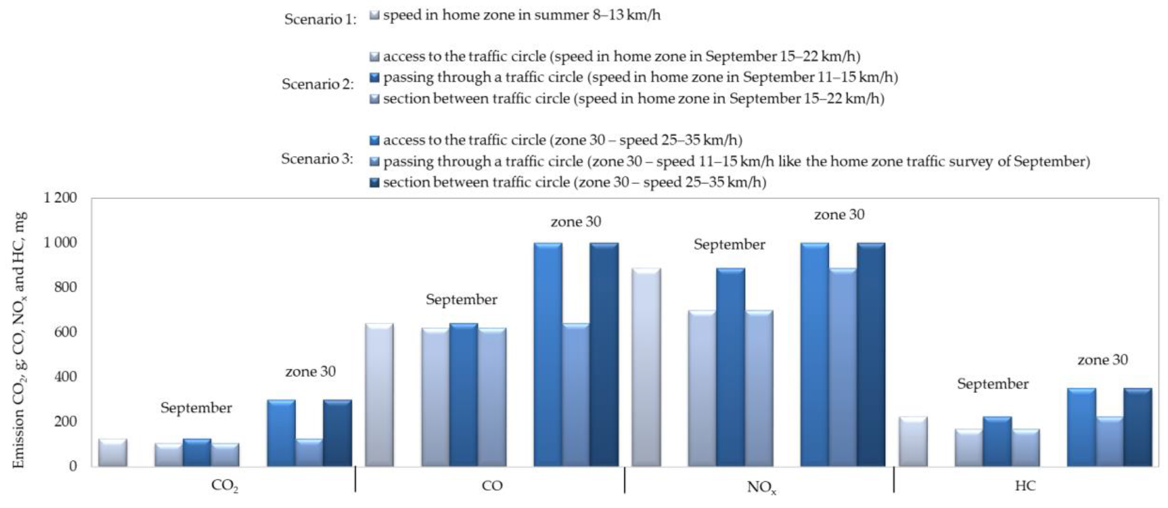
4.5. Air Pollution in Three Traffic Scenarios—Research Hypothesis H3
4.6. Fuel Consumption in Three Traffic Scenarios
5. Conclusions
- −
- The traffic calming effect and the amount of speed reduction due to traffic circles depend, to a large extent, on the height of the raised central island Δh. The resulting values of R2 (v85) = 0.85 and R2 (vav) = 0.72 indicate that 85% or 72% of the dependent variable variation (v85, vav) may be explained by a relationship with the independent variable (Δh). Now, the remaining 15% or 28% of the variability should be attributed to the effect of other relevant factors (traffic circle location, place in the sequence, street function and the surrounding streetscape features), and other random factors.
- −
- The transverse slope of the central island should be determined in a prior analytical study and implemented in the home zone design, taking into account the following factors:
- travel lane width,
- distance between the start and end of the on-street parallel parking spaces and the side street edge,
- spacing distance between subsequent traffic circles,
- the surrounding features, such as the locations and opening hours of markets, restaurants and public amenities throughout all seasons of the year.
- −
- The research findings and verification of the formulated research hypotheses show that, for main promenades lined with many retail outlets (seasonal, generating high pedestrian traffic in summer) in home zones located in spa villages, Δh values should be moderate, i.e., max. 8–10 cm. This value may be increased to max. 11–12 cm in other streets with smaller pedestrian traffic and a smaller number of retail businesses and other outlets. In turn, much greater Δh values should be applied in primarily vehicular streets that are not lined with retail businesses or other outlets and have much lighter pedestrian traffic. These higher values of Δh recommended for the above-described type of street may, for example, ranging from 17–19 cm when, past the traffic circle, the street runs for another 150 m or more. For shorter remaining street lengths, such as 50–100 m, Δh should preferably range between 14–16 cm.
- −
- When the traffic calming areas are designed in line with sustainability principles, allowing for extensive use of the carriageway space by pedestrian traffic, as is the case in this article, one-way traffic should be the first option, and green street/infrastructure components should be used, as far as practicable, for beautification reasons.
- −
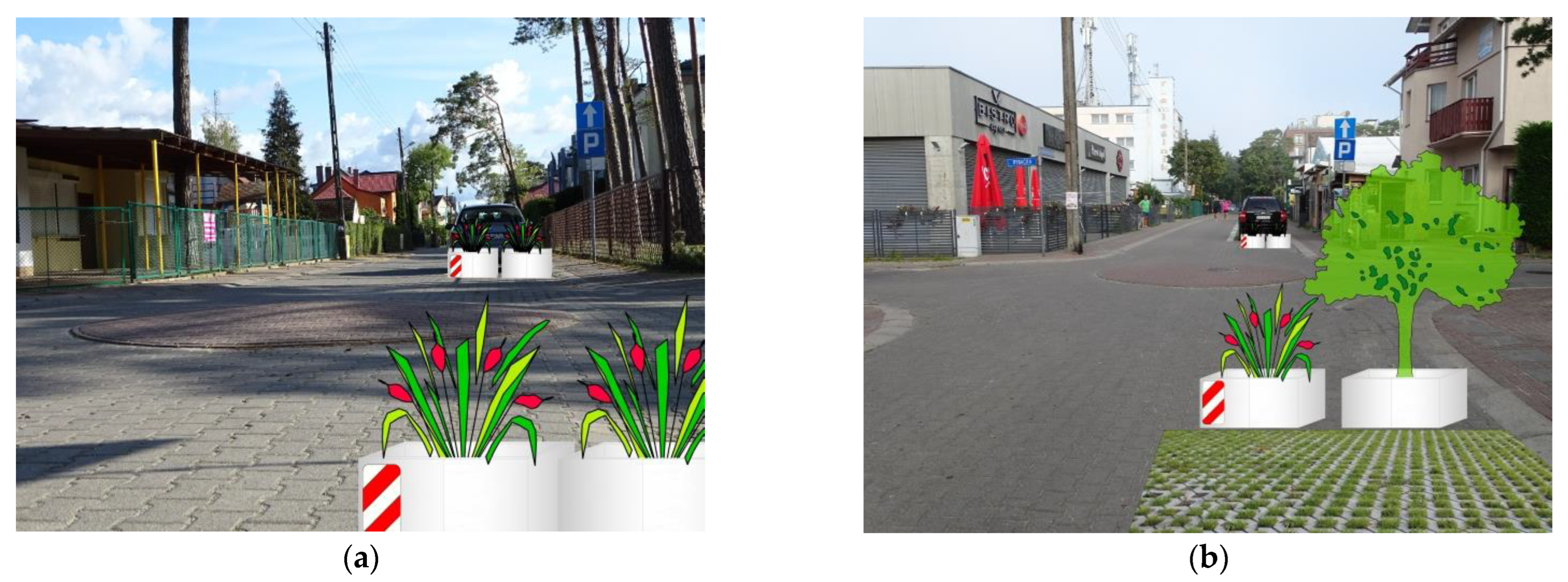
- In order to prevent exceeding of the desired speed range on the sections between traffic circles, encouraged by a lack of vehicles parked on the street, fixed-type side obstacles should be designed at the beginning and end of such sections. These obstacles include flowerbeds, planters, and concrete or wooden tree boxes, as shown in Figure A1 in Appendix A.
- −
- Finally, the authors believe that the issue of increased fuel consumption due to driving in lower gears in traffic calmed areas, such as home zones, may be effectively resolved by the global transition to electric vehicles and sustainable design of traffic calming projects.
Author Contributions
Funding
Institutional Review Board Statement
Informed Consent Statement
Data Availability Statement
Acknowledgments
Conflicts of Interest
Appendix A

References
- Horn, B.E.; Jansson, A.H.H. Traffic safety and environment: Conflict or integration. Int. Assoc. Traffic Saf. Sci. IATSS Res. 2000, 24, 21–29. [Google Scholar]
- Boglietti, S.; Tiboni, M. Analyzing the criticalities of public spaces to promote sustainable mobility, XXV International Conference Living and Walking in Cities—New scenarios for safe mobility in urban areas (LWC 2021), 9-10 September 2021, Brescia, Italy. Transp. Res. Procedia 2022, 60, 172–179. [Google Scholar] [CrossRef]
- Paszkowski, Z. Miasto Idealne w Perspektywie Europejskiej z jego Związki z Urbanistyką Współczesną; Towarzystwo Autorów i Wydawców Prac Naukowych UNIVERSITAS: Kraków, Poland, 2011. (In Polish) [Google Scholar]
- Paszkowski, Z. Historia Idei Miasta od Antyku do Renesansu; Zachodniopomorski Uniwersytet Technologiczny w Szczecinie: Szczecin, Poland, 2015. (In Polish) [Google Scholar]
- Google Earth. Available online: http://www.earth.google.com (accessed on 2 September 2023).
- Mell, I.; Clement, S. Progressing Green Infrastructure planning: Understanding its scalar, temporal, geo-spatial and disciplinary evolution. Impact Assess. Proj. Apprais. 2020, 38, 449–463. [Google Scholar] [CrossRef]
- Meerow, S. A green infrastructure spatial planning model for evaluating ecosystem service tradeoffs and synergies across three coastal megacities. Environ. Res. Lett. 2019, 14, 125011. [Google Scholar] [CrossRef]
- Learn about Green Streets. Available online: https://www.epa.gov/G3/learn-about-green-streets (accessed on 18 July 2023).
- Green Streets, Residential Streets Commercial Streets Arterial Streets Alleys. A Conceptual Guide to Effective Design Solutions; United States Enviromental Ptotection Agency US EPA Region 3: Philadelphia, PA, USA, 2009. Available online: https://nepis.epa.gov/Exe/ZyPDF.cgi/P10059Y4.PDF?Dockey=P10059Y4.PDF (accessed on 18 July 2023).
- WHO. Pedestrian Safety: A Road Safety Manual for Decision-Makers and Practitioners; WHO: Geneva, Switzerland, 2013. [Google Scholar]
- Slootmans, F. European Road Safety Observatory Facts and Figures—Pedestrians; European Commission, Directorate General for Transport: Brussels, Belgium, 2021; Available online: https://road-safety.transport.ec.europa.eu/system/files/2023-02/ff_pedestrians_20230213.pdf (accessed on 18 July 2023).
- Slootmans, F. European Road Safety Observatory Facts and Figures—Urban Areas; European Commission, Directorate General for Transport: Brussels, Belgium, 2022; Available online: https://road-safety.transport.ec.europa.eu/system/files/2022-07/ff_roads_inside_urban_areas_20220707.pdf (accessed on 18 July 2023).
- Bigazzi, A.Y.; Rouleau, M. Can traffic management strategies improve urban air quality? A review of the evidence. J. Transp. Health 2017, 7, 111–124. [Google Scholar] [CrossRef]
- Harris, G.J.; Stait, R.E.; Abbott, P.G.; Watts, G.R. Traffic Calming: Vehicle Generated Noise and Ground-Borne Vibration Alongside Sinusoidal, Round-Top and Flat-Top Road Humps; TRL Report 416; Transport Research Laboratory: Crowthorne, Berkshire, UK, 1999; Available online: https://trl.co.uk/uploads/trl/documents/TRL416.pdf (accessed on 18 July 2023).
- Lu, X.; Kang, J.; Zhu, P.; Cai, J.; Fei Guo, F.; Zhang, Y. Influence of urban road characteristics on traffic noise. Transp. Res. Part D Transp. Environ. 2019, 75, 136–155. [Google Scholar] [CrossRef]
- McAlexander, T.P.; Gershon, R.R.; Neitzel, R.L. Street-level noise in an urban setting: Assessment and contribution to personal exposure. Environ. Health 2015, 14, 18. [Google Scholar] [CrossRef]
- Ahn, K.; Rakha, H. A field evaluation case study of the environmental and energy impacts of traffic calming. Transp. Res. Part D Transp. Environ. 2009, 14, 411–424. [Google Scholar] [CrossRef]
- Yang, X.; McCoy, E.; Hough, K.; de Nazelle, A. Evaluation of low traffic neighbourhood (LTN) impacts on NO2 and traffic. Transp. Res. Part D Transp. Environ. 2022, 113, 103536. [Google Scholar] [CrossRef]
- Cloke, J.; Boulter, P.; Davies, G.P.; Hickman, A.J.; Layfield, R.E.; McCrae, I.S.; Nelson, P.M. Traffic Management and Air Quality Research Programme; TRL Report 327;Transport Research Laboratory: Crowthorne, Berkshire, UK, 1998. [Google Scholar]
- Vardoulakis, S.; Kettle, R.; Cosford, P.; Lincoln, P.; Holgate, S.; Grigg, J.; Kelly, F.; Pencheon, D. Local action on outdoor air pollution to improve public health. Int. J. Public Health 2018, 63, 557–565. [Google Scholar] [CrossRef] [PubMed]
- Burns, J.; Boogaard, H.; Polus, S.; Pfadenhauer, L.M.; Rohwer, A.C.; van Erp, A.M.; Turley, R.; Rehfues, E.A. Interventions to reduce ambient air pollution and their effects on health: An abridged Cochrane systematic review. Environ. Int. 2020, 135, 105400. [Google Scholar] [CrossRef]
- Merkisz, J.; Pielucha, J.; Fuć, P.; Nowak, M. Assessment of vehicle emission indicators for diverse urban microinfrastructure. Combust. Engines 2013, 154, 787–793. [Google Scholar]
- Kuss, P.; Nicholas, K.A. A dozen effective interventions to reduce car use in European cities: Lessons learned from a meta-analysis and transition management. Case Stud. Transp. Policy 2022, 10, 1494–1513. [Google Scholar] [CrossRef]
- Mass Hingway. Traffic Calming and Traffic Management, Chapter 16; Mass Hingway: Winchester, MA, USA, 2006. Available online: https://www.winchester.us/DocumentCenter/View/4073/MassDOT-Traffic-Calming-and-Traffic-Management (accessed on 18 July 2023).
- Traffic Calming Guidelines Chapter 6; Devon County Council, Engineering and Planning Department: Devon, UK, 1995.
- Roads Development Guide; East Ayrshire, Strathclyde Regional Council London: Kilmarnock, UK, 2010.
- Traffic Calming, Local Transport Note 1/07; Department for Regional Development (Northern Ireland): Newry, Ireland; Scottish Executives, Welsh Assembly Government: London, UK, 2007.
- Webster, P. Traffic Calming—Design Guide, Nottinghamshire County Council; Department for Transport: Nottingham, UK, 2004. [Google Scholar]
- OMGEVING cvba. IPOD, Richtlijnen, Dimensioneringen, Statuten en Checklist Voor het Openbaar Domein in Gent; OMGEVING cvba: Berchem-Antwerpia, The Neterlands, 2011. [Google Scholar]
- Vejdirektoratet, Urban Traffic Areas—Part 7—Speed Reducers; Vejdirektoratet-Vejregeludvalget: Copenhagen, Denmark, 1991.
- Lárus, Á.L. Techniques of Speed Reduction—Danish Experiences; ICTCT International Co-operation on Theories and Concepts in Traffic Safety No. 277/99; ICTCT: Copenhagen, Denmark, 1999. [Google Scholar]
- Traffic Calming Guidelines TCG; Devon County Council, Engineering and Planning Department: Devon, UK, 1991.
- Directives for the Design of Urban Roads; RASt 06; Road and Transportation Research Association (FGSV): Köln, Germany, 2006.
- Ignaccolo, M.; Zampino, S.; Maternini, G.; Tiboni, M.; Leonardi, S.; Inturri, G.; Le Pira, M.; Elena Cocuzza, E.; Distefano, N.; Giuffrida, N.; et al. How to redesign urbanized arterial roads? The case of Italian small cities. In Proceedings of the XXV International Conference Living and Walking in Cities—New scenarios for Safe Mobility in Urban Areas (LWC 2021), Brescia, Italy, 9–10 September 2021. [Google Scholar] [CrossRef]
- Are Roundabouts and Traffic Circles the Same? The Answer Might Surprise You. Available online: https://www.motorbiscuit.com/roundabouts-traffic-circles-same-answer-surprise (accessed on 18 July 2023).
- Traffic Circles and Roundabouts. Available online: https://www.surrey.ca/services-payments/parking-streets-transportation/roads-in-surrey/traffic-circles-and-roundabouts (accessed on 18 July 2023).
- Melton, L.; Shumard, D. Mini Roundabouts and Neighborhood Traffic Circles; NCTCOG Public Works Roundup, City Council Regular Meeting: Burleson, TX, USA, 21 May 2019; Available online: https://www.nctcog.org/getmedia/57bdd772-1d6b-4d1f-a344-94ab249ec392/2019PWR-MiniRAB-FINAL.pdf (accessed on 18 July 2022).
- Rao, P.S.N.; Bhagwati, S.; Satish Khanna, S. City Level Projects: Street Design Guidelines; Delhi Urban Art Commission: Delhi, India, 2020. [Google Scholar]
- System Ewidencji Wypadków i Kolizji. Available online: https://sewik.pl/ (accessed on 18 July 2023).
- Speed Displays Traffic Detection, Radar, Detection, Software; Vitronic: Kędzierzyn Koźle, Poland, 2015.
- Transportation Research Board Highway. Capacity Manual HCM 2000; Transportation Research Board TRB: Washington, DC, USA, 2000. [Google Scholar]
- Künzler, P.; Dietiker, J.; Steiner, R. Nachhaltige Gestaltung von Verkehrsräumen im Siedlungsbereich, Grundlagen für Planung, Bau und Reparatur von Verkehrsräumen; Herausgegeben vom Bundesamt für Umwelt BAFU: Bern, Switzerland, 2011; Available online: https://www.bafu.admin.ch/dam/bafu/de/dokumente/luft/uw-umwelt-wissen/nachhaltige_gestaltungvonverkehrsraeumenimsiedlungsbereich.pdf (accessed on 12 August 2023).
- Faheem, H. Suitability of existing traffic calming measures for use on some highways in Egypt. In Proceedings of the 9th International Conference on Civil and Architecture Engineering, Cairo, Egypt, 29–31 May 2012; Available online: https://iccae.journals.ekb.eg/article_44388.html (accessed on 2 September 2023). [CrossRef]
- Wirksamkeit Geschwindigkeitsdämpfender Maßnahmen Außerorts; Hessisches Landesamt für Straßen-und Verkehrswesen: Hessen, Germany. 1997. Available online: https://docplayer.org/57666796-Wirksamkeit-geschwindigkeitsdaempfender-massnahmen.html (accessed on 2 August 2020).
- Distefano, N.; Leonardi, S. Evaluation of the benefits of traffic calming on vehicle speed reduction. Civ. Eng. Archit. 2019, 7, 200–214. [Google Scholar] [CrossRef]
- Centre for Research and Contract Standardization in Civil Engineering (CROW). Recommendations for Traffic Provisions in Built-Up Areas: ASVV; CROW: Ede, The Netherlands, 1998. [Google Scholar]
- Department for Transport (DfT). Home Zones: Challenging the Future of Our Street; Department for Transport (DfT): London, UK, 2005. [Google Scholar]
- Gharehbaglou, M.; Khajeh-Saeed, F. Woonerf: A Study of Urban Landscape Components on Living Streets. MANZAR 2018, 10, 40–49. [Google Scholar] [CrossRef]
- Van den Boomen, T. Wed Met de Regels! Het Nieuwe Woonerf (Away with the Rules! he New Woonerf). NCR Handelsblad 2002, 5. [Google Scholar]
- Collarte, N. The Woonerf Concept. Rethinking a Residential Street in Somerville, Master of Arts in Urban and Environmental Policy and Planning MA (857), Tufts University, 7 December 2012. Available online: https://docplayer.net/35878575-The-woonerf-concept-rethinking-a-residential-street-in-somerville-natalia-collarte-60-wadsworth-street-apt-12h-cambridge-ma-857.html (accessed on 18 July 2023).
- Clayden, A.; McKay, K.; Wild, A. Improving residential liveability in the UK: Home zones and alternative approaches. J. Urban Des. 2006, 11, 55–71. [Google Scholar] [CrossRef]
- Pérez-Acebo, H.; Ziółkowski, R.; Linares-Unamunzaga, A.; Gonzalo-Orden, H. A Series of Vertical Deflections, a Promising Traffic Calming Measure: Analysis and Recommendations for Spacing. Appl. Sci. 2020, 10, 3368. [Google Scholar] [CrossRef]
- Nina67. Consommation D’essence en Fonction de Vitesse et Rapport, Astuces-Pratiques; Article of 23 July 2015. Available online: https://www.astuces-pratiques.fr/auto-moto/consommation-d-essence-en-fonction-de-vitesse-et-rapport (accessed on 12 August 2023).


| Traffic Circle | Δh 1, m | Street Function | l1, m 2 | l2, m 3 | Streetscape Characteristics |
|---|---|---|---|---|---|
| No. 1 | 0.12 | footstreet | 190 | 150 | summer recreation area |
| No. 2 | 0.09 | footstreet | 150 | 125 | summer recreation area, small businesses open in summer |
| No. 3 | 0.17 | vehicular street | 125 | 150 | private properties |
| No. 4 | 0.16 | vehicular street | 150 | 125 | private properties |
| No. 5 | 0.11 | main promenade | 140 | 125 | small catering and small commercial facilities open in summer |
| No. 6 | 0.08 | main promenade | 135 | 140 | year-round recreation areas and catering businesses |
| No. 7 | 0.12 | main promenade | 60 | 135 | year-round shopping centre, post office, bank, etc. |
| K–S Goodness-of-Fit Test 1 | Two-Sample K–S Test 2 | Median Test 3 | ||
|---|---|---|---|---|
| Before | After | |||
| Data from the Summer | ||||
| Traffic circle No. 1 | λ = 0.76 < λα = 1.36 | λ = 0.34 < λα = 1.36 | λ = 4.05 > λα = 1.36 | χ2 = 30.3 > χα2 = 3.84 |
| Traffic circle No. 2 | λ = 0.73 < λα = 1.36 | λ = 0.58 < λα = 1.36 | λ = 4.45 > λα = 1.36 | χ2 = 38.2 > χα2 = 3.84 |
| Data from the September | ||||
| Traffic circle No. 1 | λ = 0.92 < λα = 1.36 | λ = 1.00 < λα = 1.36 | λ = 4.03 > λα = 1.36 | χ2 = 83.8 > χα2 = 3.84 |
| Traffic circle No. 2 | λ = 0.90 < λα = 1.36 | λ = 0.75 < λα = 1.36 | λ = 2.28 > λα = 1.36 | χ2 = 27.2 > χα2 = 3.84 |
| Test | Traffic Circle | ||||||
|---|---|---|---|---|---|---|---|
| No. 1 | No. 2 | No. 3 | No. 4 | No. 5 | No. 6 | No. 7 | |
| Data from Test K–S test 1 | |||||||
| Before (Summer and September) | 4.05 | 6.9 | 5.7 | 4.5 | 2.3 | 1.35 | 4.9 |
| After (Summer and September) | 7.00 | 7.2 | 7.5 | 7.7 | 7.1 | 7.3 | 7.1 |
| Data from Median test 2 | |||||||
| Before (Summer and September) | 26.6 | 167.9 | 165.5 | 174.4 | 179.7 | 166.0 | 164.5 |
| After (Summer and September) | 97.9 | 153.8 | 139.3 | 152.4 | 180.8 | 197.8 | 56.1 |
| Test | Analysis of Traffic Circles Located along the Main Streets | |||
|---|---|---|---|---|
| No. 1 and 2 | No. 3 and 4 | No. 5 and 6 | No. 6 and 7 | |
| Data from Test K–S test 1 | 4.1 | 1.1 | 1.6 | 3.3 |
| Data from Median test 2 | 48.4 | 3.6 | 8.0 | 67.6 |
| Test | Analysis of Traffic Circle Located on Parallel Side Streets | |||
|---|---|---|---|---|
| No. 1 and 7 | No. 2 and 5 | No. 3 and 5 | No. 4 and 7 | |
| Data from Test K–S test 1 | 4.3 | 1.32 | 2.1 | 1.6 |
| Data from Median test 2 | 83.8 | 8.6 | 8.7 | 15.7 |
Disclaimer/Publisher’s Note: The statements, opinions and data contained in all publications are solely those of the individual author(s) and contributor(s) and not of MDPI and/or the editor(s). MDPI and/or the editor(s) disclaim responsibility for any injury to people or property resulting from any ideas, methods, instructions or products referred to in the content. |
© 2023 by the authors. Licensee MDPI, Basel, Switzerland. This article is an open access article distributed under the terms and conditions of the Creative Commons Attribution (CC BY) license (https://creativecommons.org/licenses/by/4.0/).
Share and Cite
Majer, S.; Sołowczuk, A. Traffic Circle—An Example of Sustainable Home Zone Design. Sustainability 2023, 15, 16751. https://doi.org/10.3390/su152416751
Majer S, Sołowczuk A. Traffic Circle—An Example of Sustainable Home Zone Design. Sustainability. 2023; 15(24):16751. https://doi.org/10.3390/su152416751
Chicago/Turabian StyleMajer, Stanisław, and Alicja Sołowczuk. 2023. "Traffic Circle—An Example of Sustainable Home Zone Design" Sustainability 15, no. 24: 16751. https://doi.org/10.3390/su152416751