A Wind Power Scenario Generation Method Based on Copula Functions and Forecast Errors

Abstract

The scenario of renewable energy generation significantly affects the probabilistic distribution system analysis. To reflect the probabilistic characteristics of actual data, this paper proposed a scenario generation method that can reflect the spatiotemporal characteristics of wind power generation and the probabilistic characteristics of forecast errors. The scenario generation method consists of a process of sampling random numbers and a process of inverse sampling using the cumulative distribution function. In sampling random numbers, random numbers that mimic the spatiotemporal correlation of power generation were generated using the copula function. Furthermore, the cumulative distribution functions of forecast errors according to power generation bins were used, thereby reflecting the probabilistic characteristics of forecast errors. The wind power generation scenarios in Jeju Island, generated by the proposed method, were analyzed through various indices that can assess accuracy. As a result, it was confirmed that by using the proposed scenario generation method, scenarios similar to actual data can be generated, which in turn allows for preparation of situations with a high probability of occurrence within the distribution system.

1. Introduction

1.1. Background

Efforts are being made in the power industry to expand renewable energy sources for sustainable environmental protection. However, since renewable energy has intermittent and fluctuating characteristics, renewable energy resources can cause various problems in the system, such as frequency dips and voltage fluctuations [1]. Therefore, it is essential to analyze the system and prepare for these problems.

There are two ways to analyze the system with renewable energy uncertainty: deterministic analysis and probabilistic analysis [2]. Before renewable energy sources were interconnected, the distribution system operated similarly, allowing for accurate predictions of future distribution system conditions through deterministic analysis. However, with the expansion of renewable energy sources, it has become impossible to predict the distribution system accurately. In this situation, to operate the system stably, deterministic distribution system analysis must assume the worst scenario [3]. However, if the worst scenario is assumed, it must consider a situation with very low probability. This will lead to significant economic losses in enhancing the power facilities. Therefore, probabilistic distribution system analysis was proposed to analyze the scenarios of high probability of occurrence.

The probabilistic distribution system analysis method generates scenarios probabilistically and derives the analysis results of the distribution system based on these. The results of this probabilistic distribution system analysis are directly influenced by the scenarios. Therefore, an accurate system analysis requires scenarios that reflect the probabilistic characteristics of historical data. For example, temporal and spatial correlations should be considered when generating wind power generation scenarios. Since wind is continuous in time and space, there are correlations between neighboring time intervals and among neighboring wind power sources [4]. In addition, since forecast models inherently entail prediction errors, the prediction errors of the forecast model should be considered. Hence, considering the spatiotemporal correlation of wind power and the prediction errors can improve the accuracy of wind power scenarios [5]. As a result, the system analysis based on these scenarios allows the uncertainty in forecasts to be quantified and the most likely situations to be analyzed [6]. In this manner, the paper proposes an improved method of generating power generation scenarios. This method will serve as the foundation for advancing sustainable distribution system analysis technology. Through this advancement, it will be possible to operate the distribution system interconnected with renewable energy sources stably.

1.2. Literature Survey

Probabilistic system analysis is based on the creation of renewable energy scenarios. Various methods are used to generate scenarios that account for uncertainties of renewable energies. Among them, sampling-based scenario generation methods, including the Monte Carlo sampling method, the Latin hypercube sampling method, and the copula-based sampling method [7], have been widely used.

The Monte Carlo sampling method uses probability distributions derived from historical data and random numbers to generate samples [8]. The Monte Carlo sampling method is a commonly used scenario generation method thanks to its simplicity and computational efficiency [9]. Hence, numerous studies have employed the method for scenario generation across diverse research objectives. In [10], a Monte Carlo sampling method was used to generate scenarios of wind power generation, which were used to evaluate the security of the wind generators interconnected to power systems. The authors of [11] also applied the Monte Carlo sampling method to generate wind power scenarios to forecast wind power ramps. Furthermore, the authors [12] sampled the harmonic of the electric vehicle charging station using the Monte Carlo method and, based on this, analyzed the impact on the distribution system of the electric vehicle charging station. Owing to the versatility of the Monte Carlo sampling method, it can be applied to conduct diverse stability studies, including small signal stability analysis, transient stability analysis, and voltage stability analysis [13]. In [14], the Monte Carlo sampling method was used to create scenarios of wind power generation, and the small signal stability of the power system was analyzed through Monte Carlo simulations and the probabilistic analysis. Moreover, in [15], the Monte Carlo method was used to model the uncertainty of load and PV power sources and probabilistically derived indicators such as reactive power margin to analyze voltage stability. However, the Monte Carlo sampling method generates irregular random samples. Accordingly, there may be scenarios that are not considered or, conversely, scenarios that are considered multiple times. To address these limitations, methods have been proposed to generate scenarios uniformly. The authors of [16] improved the scenario generation using a quasi-Monte Carlo method that samples with patterned rather than random numbers.

The Latin hypercube sampling method is similar to the quasi-Monte Carlo method in that it generates uniform samples. Its difference from Monte Carlo sampling is that the Latin hypercube sampling method uses a cumulative distribution function with equally spaced bins. Samples are generated at each bin, ensuring all bins are sampled uniformly [17]. The authors of [18] modeled renewable energy generation using the Latin hypercube sampling technique and evaluated the voltage stability. In [19], the two variables of wind power generation and system load were modeled through Latin hypercube sampling, from which the probabilistic voltage profile was derived and used to execute the optimal placement of wind turbines. To enhance the Latin hypercube method, the authors of [20] proposed an extended Latin hypercube sampling method that iterates the sample generation until the sample converges to a value. However, the Monte Carlo sampling method and the Latin hypercube sampling method can only generate independent probability distributions of variables, not probability distributions that reflect correlations of variables. For accurate scenario creation, it is crucial to consider the correlations among variables when generating scenarios.

The copula-based sampling method can reflect the correlation among variables in a scenario. A copula function is a function that derives a probability distribution function of multiple correlated variables [21], and copula-based sampling methods have been studied extensively. In [22], power sources with uncertainties were modeled using Gaussian and Gumbel copula functions, and based on the analysis of active and reactive power within the system, a voltage-var scheme was optimized. Furthermore, the authors of [23] generated scenarios by considering the correlation of wind power generation over 24 h through a copula function. In this paper, the Gaussian copula function was used, but to account for tail dependence between variables, the Vine copula function was used [24]. The authors of [25] used the Vine copula function to account for the spatiotemporal correlation of wind power generation in scenario generation, which improved the accuracy of voltage and current analysis. However, these papers did not consider the forecast errors of the forecast model in the scenario generation process.

By generating samples using the probability distribution function of the forecast errors and adding them to forecasted values, forecast errors can be offset. Hence, this work proposes an accurate method that considers the spatiotemporal correlation of variables and the forecast errors of the forecasting model simultaneously.

1.3. Contributions

The purpose of this work is to create wind power scenarios with high accuracy, ensuring that the scenarios generated closely align with the stochastic characteristics of the actual data while maintaining minimal deviation from the actual data. The contributions of this paper are as follows.

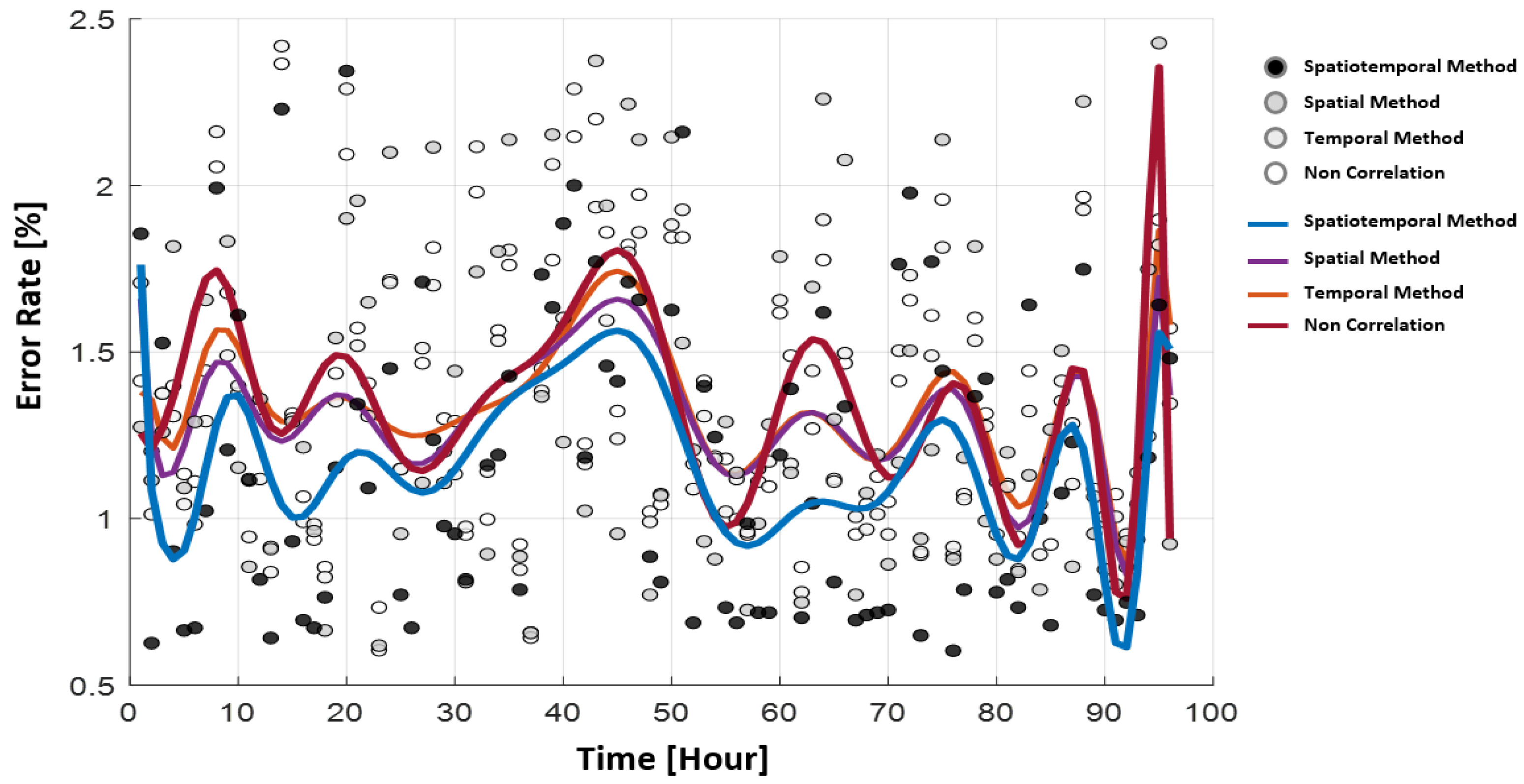
• This study proposes a methodology that creates wind power scenarios, considering temporal and spatial correlations, which improves the accuracy of scenario generation. It also solves the problem of computational complexity that arises when temporal and spatial correlation are considered simultaneously.
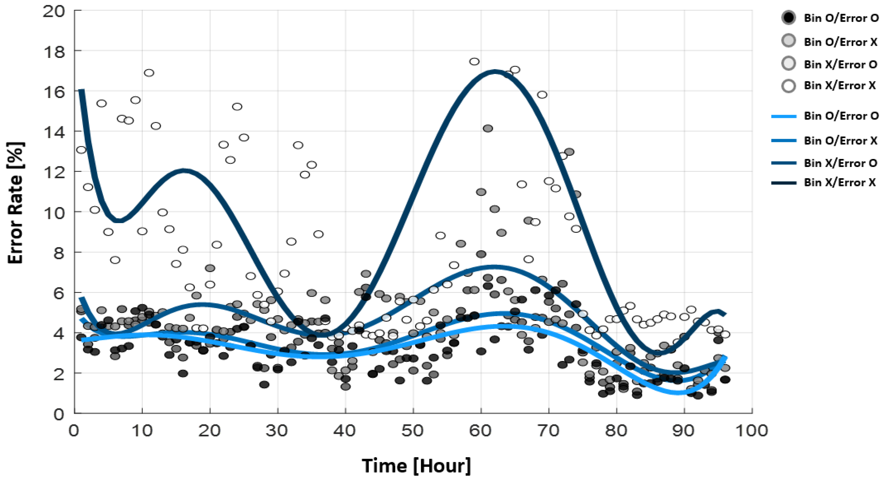
• This study models forecast errors in the scenario generation process to enhance the forecast accuracy.
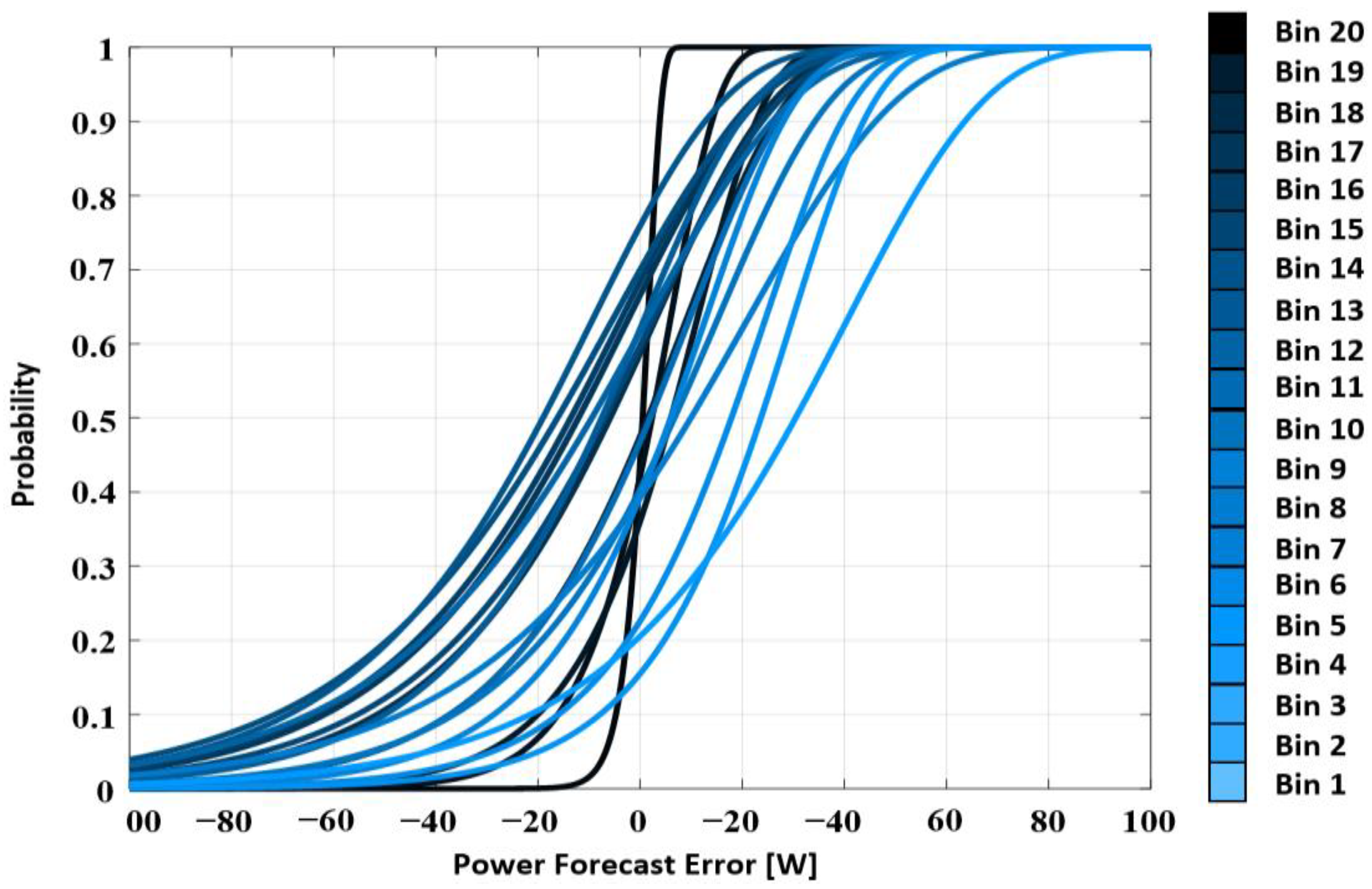
• This study analyses the stochastic properties of forecast errors in different generation bins and reveals that the stochastic properties differ among bins. Applying the result to scenario generation makes it possible to offset the forecast errors with a high probability of occurrence.
• The probabilistic analysis can utilize the scenarios generated by the proposed method to improve its reliability, eventually enhancing the efficiency and reliability of power system operation.

2. Proposed Methodology

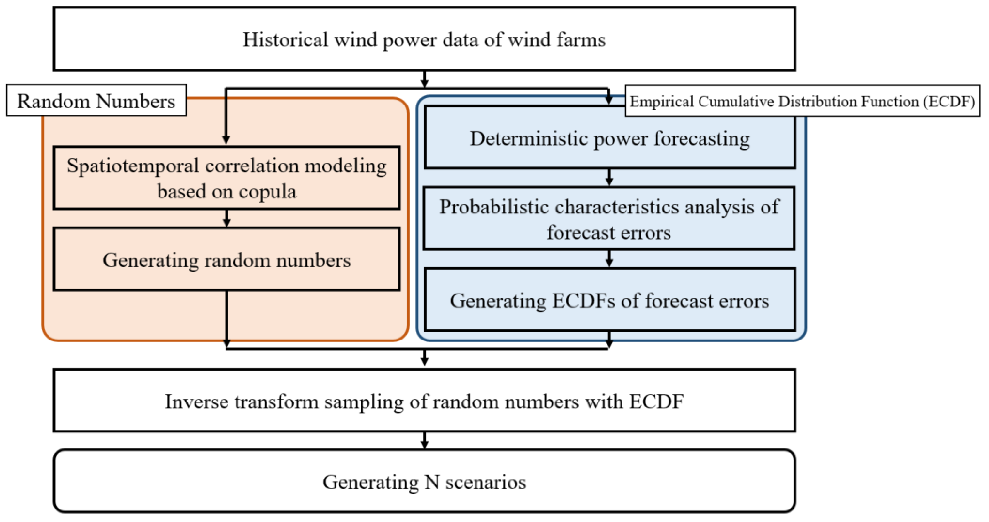
2.1. Wind Power Scenario Generation Method

The probabilistic scenario generation process consists of two processes: generating random numbers and inversely sampling the random numbers with a cumulative distribution function. When generating random numbers, a copula function reflects the spatial and temporal correlation of wind power generation. The cumulative distribution function of the forecast error is used to compensate for the forecast error during inverse sampling. Figure 1 illustrates the scenario generation process.

2.2. Generating Spatiotemporally Correlated Random Numbers

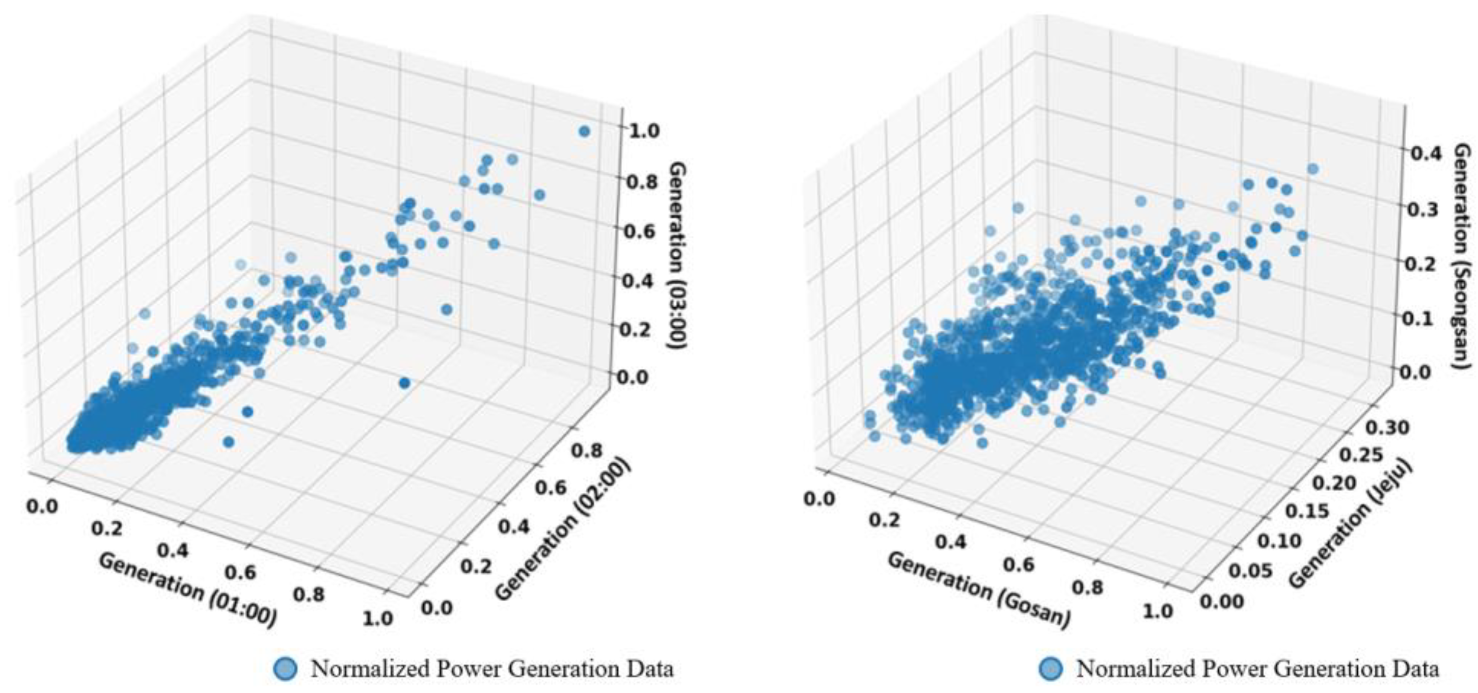
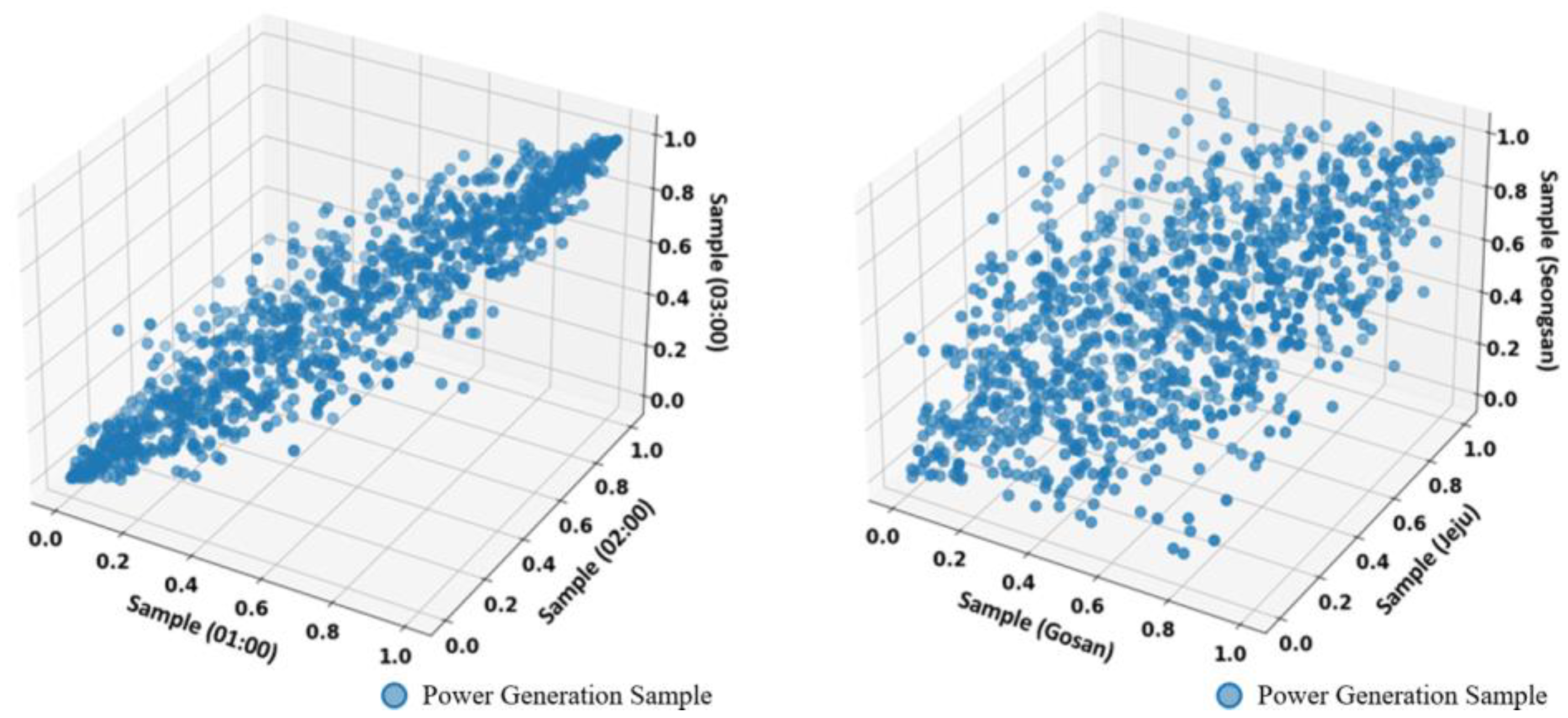
2.2.1. Generating Spatial and Temporal Samples Using Copula Function

The wind is continuous in time and space, and accordingly, wind power generation is correlated in time and space. Therefore, the spatiotemporal correlation of the wind should be considered to improve the accuracy of the scenario generation method. This correlation can be reflected in the copula function, which derives a joint probability density function through the relationships among the probability distributions of variables. The joint probability density function for $X=(x_1,\dots ,x_d)$ in d-dimensions is given by Equation (1).

$$f\left(x_1,\dots ,x_d\right)=c(F_1\left(x_1\right),\dots ,F_d(x_d)){\prod }_{i=1}^d{f}_i\left(x_i\right)$$

(1)

where $x_1,\dots ,x_d$ are the random variables, $c$ is the copula function, $F_1\left(x_1\right),\dots ,F_d\left(x_d\right)$ are the marginal probability distribution functions of variables, and $f_i\left(x_i\right)$ are the marginal probability density function of variables.

To estimate the copula density function, the log-likelihood function is used. The log-likelihood function is derived by taking the logarithm of the likelihood function and is used to estimate the parameters in order to find the most fitting probability density function for the given data. Initially, the parameters that maximize the log-likelihood function are estimated to derive the parameters for each marginal probability density function. Based on these parameters, the parameters that maximize the log-likelihood function are estimated to determine the parameters of the copula function that maximize the copula probability density function. This allows for the estimation of the joint density function.

Through the method described above, the random numbers that reflect spatiotemporal correlation can be generated. Since the spatial and temporal correlations increase dimensions, the accuracy of the scenarios may decrease. Hence, each sample for temporal and spatial correlations is generated separately. A temporally correlated wind power sample matrix is generated by Equation (2), followed by creating a spatially correlated wind power sample matrix based on Equation (3). Then, the temporal and spatial sample matrices are integrated into the spatiotemporal samples.

$$f\left(x_{m,1},\dots ,x_{m,T}\right)=c(F_{m,1}\left(x_{m,1}\right),\dots ,F_{m,T}(x_{m,T})){\prod }_{t=1}^T{f}_{m,t}(x_{m,t})$$

(2)

$$f\left(x_1,\dots ,x_M\right)=c(F_1\left(x_1\right),\dots ,F_M(x_M)){\prod }_{m=1}^M{f}_m(x_m)$$

(3)

where $x_{m,1},\dots ,x_{m,e}$ are the wind power generations of the m-th wind turbine over time $t$, indicating the data for the entire $T$ time period. $F_{m,1}\left(x_{m,1}\right),\dots ,F_{m,T}\left(x_{m,T}\right)$ are the marginal probability distribution functions of wind power generations of the m-th wind turbines over time, and $f_{m,t}\left(x_{m,t}\right)$ is the marginal probability density function of wind power generations of the m-th wind turbine at time t. Equation (2) is the copula joint probability density function of the m-th wind turbine that accounts for the temporal correlation. Assuming a total of M wind turbines, the wind power at the time t of the m-th wind turbine is set to $x_{m,t}$. The samples of the m-th wind power output for T hours are generated using Equation (2), and these samples make up the time sample matrix $T_m$, a matrix structure of N-by-T, where N is the number of scenarios to be generated.

A joint probability distribution function accounting for spatial correlations is also generated by the copula function derived from Equation (2). Because only spatial correlation is considered, the time factor t is neglected. The samples reflecting the spatial correlations are generated using the derived joint probability distribution function. These samples make up a spatial sample matrix, $S$, and the matrix has an N-by-M structure.

2.2.2. Generating Spatiotemporal Samples

The samples, generated by temporal and spatial correlations separately, are integrated, becoming samples with spatiotemporal correlations. This method involves multiplying the elements of the two matrices $T_m$ and $S$. Each column of the two matrices has a uniform distribution between zero and one; therefore, each correlation is preserved after the integration. The integration process includes the following steps.

(1)

The temporal wind power samples of each wind turbine are generated using the copula function and are used to create M matrices, $T_1, T_2,$⋯,$T_M$. The n-th row of the m-th sample matrix $T_M$ has the elements $t_{n1},t_{n2},\cdots ,t_{nT}$.

(2)

Neglecting the time series correlation of the wind power, the matrix $S$, representing the spatial correlation among the wind power plants, is generated using the copula function. Its element, $s_{nm}$, indicates the n-th row element of the m-th sample matrix S.

(3)

The random number samples are generated by multiplying the n-th row of the matrix $T_m$ and the n-th row and m-th column elements of the matrix $S$. The random number samples are generated as ($s_{nm}{t}_{n1},s_{nm}{t}_{n1},\dots , s_{nm}{t}_{n1}$). This process is repeated (N × M × T) times to generate the final wind power samples.

The final samples are created from the M matrices with a structure of N-by-T. Each sample matrix represents T-hour samples of each wind turbine. The generated sample values are fitted to the actual values by applying inverse transform sampling to the empirical cumulative distribution function (ECDF) generated with historical data.

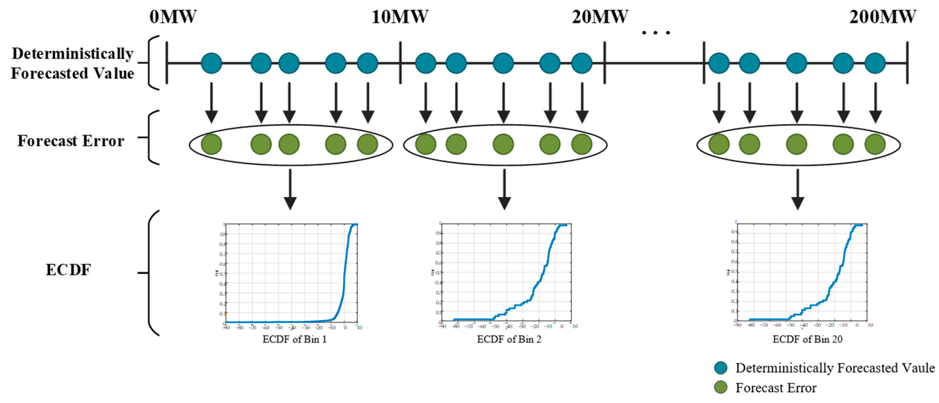
2.3. Generating ECDFs Based on the Errors of a Forecast Model

Generally, the deterministic forecast models of wind power generation have forecast errors. The probabilistic properties of these forecast errors can vary depending on the magnitude of the power generation. In other words, the probability distribution of the forecast errors in a particular bin of power generation is different from the probability distribution of other bins.

Figure 2 illustrates the cumulative probability distribution function of the forecast errors for each bin, indicating that the cumulative probability distribution functions differ by generation bins. It also shows that the mean is roughly zero for all generation bins. However, the standard deviations of the forecast errors change significantly with the magnitude of the generation. In other words, most of the forecast errors are close to zero for a large magnitude of generation, but the forecast error increases as the magnitude decreases. This change indicates that the forecast model is more accurate for large generations and less accurate for small ones. As a result, the stochastic properties of the forecast errors change with the magnitude of the generation, and thus, the properties should be considered when creating scenarios.

The process of generating empirical cumulative distribution functions is depicted in Figure 3. The magnitude of the power generation is divided into bins. When forecasting the power generation in a deterministic manner, the forecasted values (blue circles) are categorized based on the bins. The forecast errors (green circles) corresponding to these forecasted values converge within each category, and based on this, an ECDF is generated for each bin.

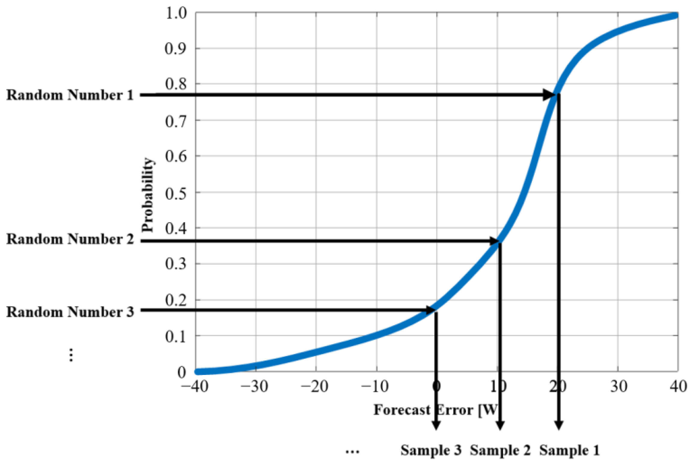
2.4. Generating Scenarios with Inverse Transform Sampling

The previous sections describe creating random numbers with spatiotemporal correlation and building ECDFs that consider the error of the forecast model. The spatiotemporally correlated random numbers are inversely sampled into the ECDFs to generate the wind power scenarios. If the deterministic forecast model predicts at a given time, the forecast will correspond to a given generation bin with an ECDF. Then, random numbers with spatiotemporal correlation are inversely sampled into this ECDF. The process of inverse transform sampling is depicted in Figure 4. Random numbers, ranging from 0 to 1, are inputted into the y-axis as probabilities. The ECDF is a function of the forecast error, and thus, the x-value where it intersects with the ECDF becomes a sample of the forecast error. Consequently, the result of the inverse sampling of random numbers becomes a forecast error, which is ultimately added to the deterministic forecasts, forming wind power scenarios. This process is repeated multiple times to generate multiple scenarios.

The ECDF is a function of the forecast errors. Hence, the inverse sampling of random numbers becomes forecast errors, which finally add to the deterministic forecasts, forming wind power scenarios. This process is repeated several times to generate multiple scenarios.

3. Case Study and Discussion

The scenario generation method based on the spatiotemporal correlation and the forecast errors was described in the previous sections. Case studies were conducted to validate the proposed method and compare it with other methods. For that purpose, a deterministic forecast was first conducted. Using weather and power generation data measured from 1 January 2021 to 31 August 2021, in three regions of Jeju Island (i.e., Gosan, Seongsan, Jeju), the DNN and LSTM algorithms were trained. Through the DNN and LSTM algorithms, wind power generations from 1 September 2021 to 31 December 2021, were forecasted. Based on these forecasts, the stacking ensemble forecast algorithm was trained. Consequently, the wind power generations from 1 January 2022 to 28 February 2022, were forecasted through the ensemble algorithm.

After the deterministic forecast, scenario generation was performed based on the deterministic forecast values. The spatiotemporal correlation of wind power generation was first obtained through the measured wind power generation data, and random numbers were generated through this correlation. The scenarios were generated by inversely transforming these random numbers to the ECDFs of the forecast errors. Here, the forecast errors refer to the forecast error of the ensemble forecast model. As a result, the scenarios for 24 h from 1 January 2022 to 28 February 2022, for each region were generated.

3.1. Verification of Scenario Generation Method

A scenario generation method is proposed in this paper that models the probabilistic characteristics of the actual data, including spatiotemporal correlation, by utilizing the probability distribution function of power generation. Therefore, an analysis is conducted to determine how similar the probabilistic characteristics of the generated scenarios are to the actual data characteristics, using two indices. Index I compares the probability distribution function of created scenarios with that of actual data, and Index II analyzes the similarity of the spatial and temporal correlations.

Index I uses mean, standard deviation, skewness, and kurtosis. The error rates of the four values are derived by comparing the probabilistic characteristics of the scenarios with the actual data. As there were 1000 scenarios, the error rates of the 1000 scenarios were calculated. The four different probabilistic characteristics needed to be compared. The error rate for each probabilistic characteristic is calculated by comparing the probabilistic characteristics of the actual data with those of each scenario. After deriving the error rate for all scenarios, the final error rate for the probabilistic characteristics can be determined by averaging these rates—the four probabilistic characteristics all equally influence the probabilistic characteristics of the data. The error rate for each probabilistic characteristic is a value normalized to a percentage. Hence, the error rates were averaged over the four values as presented in Equation (4).

$$e\_s=\frac{1}{4}·(\left|e_{mean}\_s\right|+\left|e_{std}\_s\right|+\left|e_{kurtosis}\_s\right|+\left|e_{skewnees}\_s\right|)$$

(4)

where $e_{mean}\_s$, $e_{std}\_s$, $e_{kurtosis}\_s$, and $e_{skewnees}\_s$ are the error rate of the mean, standard deviation, kurtosis, and skewness, respectively. $e\_s$ is the average value of the error rates comparing the mean, standard deviation, skewness, and kurtosis values for the s-th wind turbine scenarios with actual data. Adding these values for all wind farms yields the Index I, as described in Equation (5). Since Index I represents the error rate, a smaller value means that the probabilistic properties of the scenarios are similar to those of the actual data.

$$Index I=\left(\frac{1}{S}·\sum _{s=1}^{S}e\_s\right)\times 100 [\%]$$

(5)

Index II compares the correlations of the scenarios with those of actual data, using Pearson correlation, calculating the error rate of the temporal correlation in each region. By comparing the spatial correlation of scenarios for all regions with the spatial correlation of the actual data, the error rate of the spatial correlation, denoted by $e_{spatial}$, is calculated. At last, Index II can be obtained by averaging the four error rates by Equation (6). The smaller the value of Index II, the more similar the spatiotemporal correlation of scenarios is to that of real data.

$$Index II=\left(\frac{1}{2}·(\frac{1}{S}·\left(\left|e_{tem{p}_1}\right|+\left|e_{tem{p}_2}\right|+\cdots +\left|e_{tem{p}_S}\right|\right)+\left|e_{spatial}\right|)\right)\times 100 [\%]$$

(6)

where $e_{temp\_gosan}$, $e_{temp\_sungsan}$, and $e_{temp\_jeju}$ are the error rates of the temporal correlations in Gosan, Seongsan, and Jeju regions, respectively.

For the assessment of how accurately scenario generation reflects the probabilistic characteristics and spatiotemporal correlation of real data, comparisons were made among the indices of scenarios generated with and without the consideration of temporal and spatial correlation. Depending on the consideration, the scenarios were categorized into uncorrelated, spatially correlated, temporally correlated, and spatiotemporally correlated scenarios. Scenarios without correlation were generated by inverse sampling from a probability distribution function of the entire historical data. The index values for scenarios with or without considering correlations are summarized in

Table 1. Indices of scenarios with and without considering correlation.

Index	Non-Correlation Method (%)	Spatial Method (%)	Temporal Method (%)	Spatiotemporal Method (%)
I	12.5058	11.9763	11.9384	11.1801
II	39.2320	39.2234	38.9961	38.9237

.

When comparing the spatially correlated scenarios with the temporally correlated scenarios, the temporally correlated scenarios have lower values in both Index I and II. This result is mainly because the real data of wind power generation are more temporally correlated than spatially correlated. This observation can be explained in Figure 5, which plots normalized wind power generations. The left plot of Figure 5 shows the temporal correlation of wind power generation at 1:00, 2:00, and 3:00, and the right one shows the spatial correlation in Gosan, Seongsan, and Jeju regions. In Figure 5, the left plot is more regularly distributed than the right one, proving that the temporal correlation of power generation data used in this case study is larger than that of the spatial correlation.

As shown in Table 1, it is evident that the reflection of spatiotemporal correlation in the scenario generation method leads to the most minimized values for Index I and Index II, which are 11.1801% and 38.9237%, respectively. The more the correlations are considered, both Index I and Index II show decreasing trends. Consequently, the method of scenario generation considering the spatiotemporal correlation is the most effective in emulating the stochastic properties and spatiotemporal correlations inherent in actual data.

To generate scenarios with spatiotemporal correlation, the method uses the time and space samples shown in Figure 6. These samples, essential to the scenario generation process, are generated by a Gaussian copula function. The temporal distribution is represented in the left plot of Figure 6, illustrating samples for different times, 1:00, 2:00, and 3:00. Meanwhile, the right plot of Figure 6 captures the distribution of the spatial samples for distinct spaces, Gosan, Seongsan, and Jeju regions. Integration of these temporally and spatially derived samples, followed by inverse transformation using ECDFs, is used for scenario generation. The left and right plots of Figure 6 are derived from the correlation in the left and right plots of Figure 5, respectively.

The scenario generation method which considers the spatiotemporal correlations, generation bins and forecast errors was explained. It has also been shown through indices that this scenario generation method captures the stochastic interdependencies in the real data. It should be verified that the scenarios generated by this method are similar to the actual data and are the accurate scenarios. This verification is achieved through an error rate—an index that measures the dissimilarity between the generated scenarios and the actual data. The error rate is derived by comparing the scenarios with the actual data.

Figure 7 and Figure 8 illustrate the error rates for scenario generation using different methods, including the results of calculating the error rate for the scenario generation across other methods, presented as individual data points. A lower error rate corresponds to a higher level of accuracy in the scenario generation method. To facilitate a visual comparison among the methods, the error rate results for a representative 96 h were shown as data points, and these data points were fitted into a curve. The curve used in this process is the 7th-degree polynomial, and the optimal polynomial was generated by finding the coefficients of the polynomial for the given data points.

Figure 7 compares the error rates of scenarios generated with and without considering temporal and spatial correlation. It can be observed from the figure that error rates decrease as the total correlation is considered. When spatiotemporal correlation is considered, the distribution of power generation over time and space converges to that of actual data. The random generation of samples without considering the temporal correlation might neglect the influence of previous time points. Similarly, the random generation of samples without considering spatial correlation leads to scenario generation independent of neighboring wind farms. Consequently, with scenario generation that considers spatial and temporal correlations based on the close time and neighboring wind farms, the similarity of distributions between the scenarios and the historical data can be improved, improving the accuracy of scenarios created.

In the meantime, Figure 8 compares the error rates of scenarios generated with and without consideration of bins and errors. Note that the proposed method considers both bins and errors. In contrast, the method without considering bins generates an ECDF for the entire data without generating an ECDF for each bin, and the method without considering errors generates scenarios by generating an ECDF for power generation instead of an ECDF for errors.

Figure 8 proves that error rates are minimized when the scenario is generated while accounting for errors and bins. Conversely, the error rates are maximized when the scenario is generated without considering errors and bins. The use of forecast errors in the prediction model can mitigate the errors by subtracting the forecast error from the deterministically predicted power generation. It has also been shown that the probability distribution of the forecast errors differs for each bin. By taking these bins into account, it becomes possible to extract the forecast errors that are more likely to occur within each bin. This extraction allows for the compensation of errors in the power generation forecast. Consequently, incorporating the forecast errors and generation bins into the scenario generation process can significantly reduce the discrepancy between the generated scenario and the actual generation.

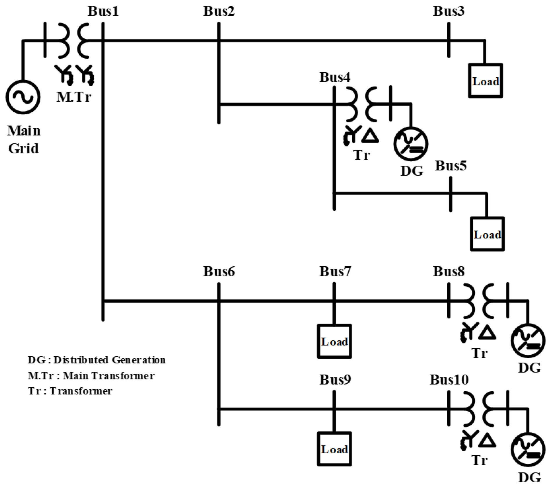
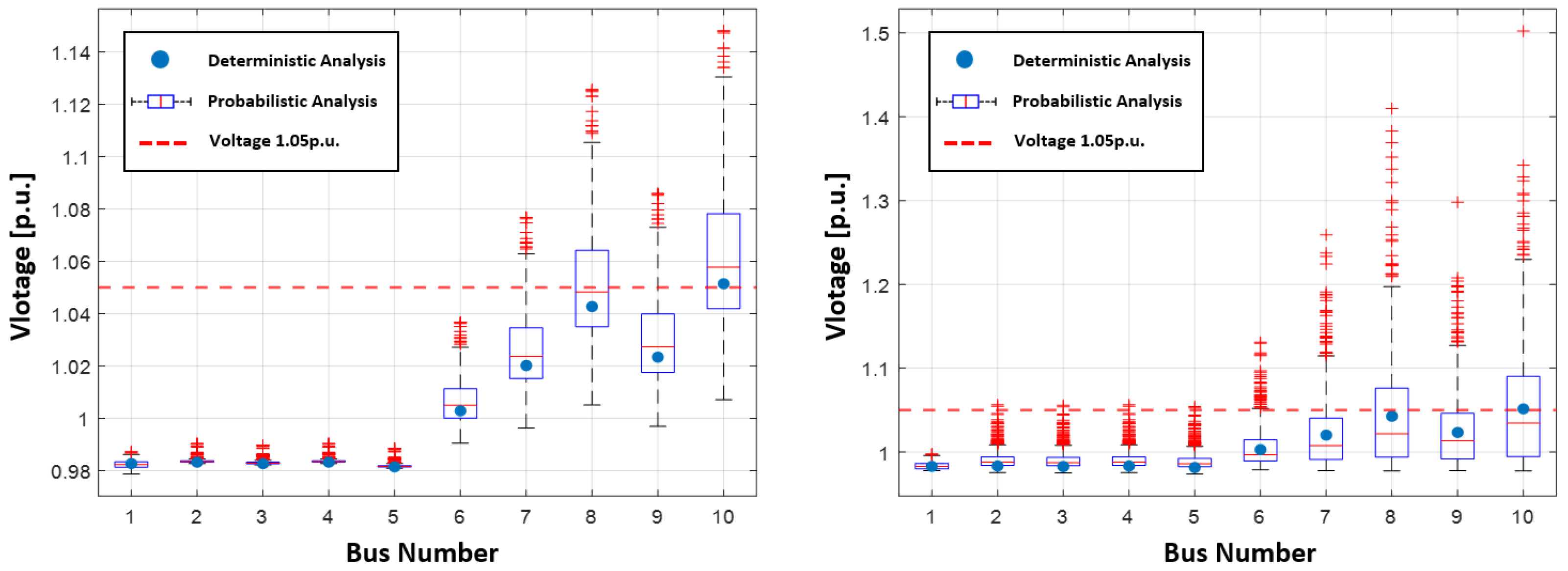
3.2. Probabilistic Distribution System Analysis

A probabilistic analysis of the distribution system was performed by inputting the generated renewable energy generation scenarios into the distribution system model. In this case study, a voltage analysis and a fault current analysis were subsequently conducted. The results of probabilistic analysis and deterministic analysis were compared. Moreover, the results of probabilistic analysis using scenarios generated by the proposed method were compared with those derived from scenarios generated by other methods.

The test system was modeled using Matlab/Simulink, as shown in Figure 9. The substation transformer, connected to the main grid, reduces voltage from 154 kV to 22.9 kV. This model represents a radial distribution system, incorporating four loads and three distributed generations. The generation scenarios of the distributed generations correspond to 1 o’clock on 1 January 2022. Each distributed generation’s output is based on the generation scenarios from Jeju, Seongsan, and Gosan areas.

The probabilistic voltage analysis of the distribution system was based on power flow analysis. The power flow analysis was iteratively executed, using the generation scenarios as input. The voltage values, derived from the recurrent power flow analyses, allow for the identification of any violations of voltage standards. Here, the voltage standard was set to 1.05 p.u.

Figure 10 shows the voltages derived from probabilistic and deterministic analyses, represented according to the bus. The results of the probabilistic voltage analysis are represented as a box plot, while the results of the deterministic voltage analysis are marked with blue dots. Furthermore, the left image in the figure represents the analysis results for the scenarios generated by the proposed method, while the right image represents the analysis results for the scenarios generated by a simple method. The scenarios generated by the simple method were derived by generating random numbers through a Gaussian normal distribution function, using the hourly average and standard deviation of past generation data. In other words, the scenario generated by the simple method did not take into account the spatiotemporal correlation and prediction error of the generation.

The deterministic analysis assessed the system to be more stable, while the probabilistic analysis showed that higher voltages could occur in the system (Figure 10 (Left)). For example, the deterministic analysis predicted a voltage violation at Bus 16, whereas the probabilistic analysis indicated the possibility of voltage violations at four different buses. The deterministic analysis has limitations in preparing for voltage violations at Buses 7, 8, 9, and 10 when the generation increases. This is due to the inability of deterministic predictions to model the variability of renewable energy. Consequently, it is confirmed that the probabilistic distribution system analysis, which takes into account the variability of renewable energy, allows for the consideration of various likely situations.

When analyzing scenarios generated by the simple method, it is observed that the range of voltage analysis results is larger (Figure 10 (Right)). In other words, the analysis based on the simple method indicates that the voltage could increase up to 1.5 p.u. Since the method uses a theoretical probability distribution function to generate a wide range of generation scenarios, it produces a wide range of distribution system analysis results. In such cases, it may be assumed that higher voltage occurs than what actually occurs in the system, leading to more system reinforcements than necessary. This could result in significant economic losses.

By performing the probabilistic distribution system analysis using scenarios as input, a comparison was made between probabilistic analysis and deterministic analysis. Since the deterministic prediction is unable to model the uncertainty of renewable energy, the deterministic analysis is proved to be unsuitable for distribution system analysis interconnected with volatile renewable energy. Furthermore, a comparison was made between the proposed scenario generation method and the simple scenario generation method. When analyzing the distribution system with scenarios generated by the simple method, the analysis results can be broadly derived, which could reduce the reliability of the results. Consequently, it was shown that by conducting the probabilistic distribution system analysis through the proposed method, it is possible to consider both the volatility of renewable energy sources and only the situations with a high probability of occurrence.

4. Conclusions

Probabilistic distribution system analysis is suitable for analyzing distribution systems with numerous interconnected renewable energy sources, as it takes into account the volatility of these sources. The probabilistic distribution system analysis is based on power generation scenarios, and these scenarios significantly impact the outcome of the probabilistic distribution system analysis. Consequently, this study has proposed a method aimed at enhancing the precision of these scenarios.

For this purpose, the spatiotemporal correlation of renewable energy generation was analyzed, and it was confirmed that there is a correlation between adjacent times and spaces. A copula function was used to create scenarios that reflect this spatiotemporal correlation. Through the copula function, a joint probability distribution function of power generation variables was derived, and scenarios with spatiotemporal correlation were generated by creating random numbers through this function. Additionally, the probabilistic characteristics of the prediction error of the power generation prediction model were analyzed, and it was confirmed that the probabilistic characteristics of prediction errors differ based on the power generation interval. To reflect these characteristics, a cumulative distribution function for prediction errors was established for each power generation interval, and scenarios were created by offsetting prediction errors by sampling random numbers through this function.

The scenario generation method was assessed through indicators that compare the probabilistic characteristics and magnitude of the power generation scenarios and the actual data. The probabilistic characteristics of the scenarios, based on the proposed method, were found to be similar to the actual data when analyzed through the indicator comparing probabilistic features. Moreover, the indicator comparing magnitudes revealed that the scenarios derived from the proposed method had minor discrepancies from the actual data. Subsequently, a probabilistic distribution system analysis was carried out using the generated scenarios as input, and the results were analyzed. When the results of the probabilistic distribution system analysis were compared with those of the deterministic distribution system analysis, the probabilistic approach, which accommodates the fluctuation of renewable energy, proved suitable for the analysis of distribution systems interconnected with renewable energy. Furthermore, when the proposed scenario generation method was compared with a simplistic method, the proposed method enabled more economical system operation by taking into account only situations with a high probability.

The scenario generation method presented in this paper will provide sustainable solutions from various perspectives. This method is capable of modeling the volatility of renewable energy sources, making it suitable for analyzing distribution systems interconnected to renewable energy sources. Therefore, through this method, even if numerous renewable energy sources are interconnected, the distribution system can be maintained stably. As a result, this method provides a sustainable solution for the expansion of renewable energy sources. In addition, this method allows for the precise analysis of future situations, such as line reconfiguration and power facility reinforcement. This allows for the provision of strategies that can minimize the cost of operating the distribution system while ensuring its stability. Ultimately, the proposed method is expected to provide a solution that can enhance the operational efficiency of the distribution system.

The authors persistently aim to improve the present techniques of probabilistic power generation forecasting and probabilistic distribution system analysis. To advance the probabilistic forecasting method, the forecasts based on various algorithms have been studied. Furthermore, various stability analyses through the forecasting method are planned to be studied by developing distribution system stability analysis techniques.

References

1. Ahmed, F.; Al Kez, D.; McLoone, S.; Best, R.J.; Cameron, C.; Foley, A. Dynamic Grid Stability in Low Carbon Power Systems with Minimum Inertia. Renew. Energy 2023, 210, 486–506. [Google Scholar] [CrossRef]
2. Beltrán, J.C.; Aristizábal, A.J.; López, A.; Castaneda, M.; Zapata, S.; Ivanova, Y. Comparative Analysis of Deterministic and Probabilistic Methods for the Integration of Distributed Generation in Power Systems. Energy Rep. 2020, 6, 88–104. [Google Scholar] [CrossRef]
3. Hasan, K.N.; Preece, R.; Milanović, J.V. Existing Approaches and Trends in Uncertainty Modelling and Probabilistic Stability Analysis of Power Systems with Renewable Generation. Renew. Sustain. Energy Rev. 2019, 101, 168–180. [Google Scholar] [CrossRef]
4. Li, Y.; Peng, X.; Zhang, Y. Forecasting Methods for Wind Power Scenarios of Multiple Wind Farms Based on Spatio-Temporal Dependency Structure. Renew. Energy 2022, 201, 950–960. [Google Scholar] [CrossRef]
5. Tu, Q.; Miao, S.; Yao, F.; Li, Y.; Yin, H.; Han, J.; Zhang, D.; Yang, W. Forecasting Scenario Generation for Multiple Wind Farms Considering Time-Series Characteristics and Spatial-Temporal Correlation. J. Mod. Power Syst. Clean Energy 2021, 9, 837–848. [Google Scholar] [CrossRef]
6. Sweeney, C.; Bessa, R.J.; Browell, J.; Pinson, P. The Future of Forecasting for Renewable Energy. Wiley Interdiscip. Rev. Energy Environ. 2020, 9, e365. [Google Scholar] [CrossRef]
7. Li, J.; Zhou, J.; Chen, B. Review of Wind Power Scenario Generation Methods for Optimal Operation of Renewable Energy Systems. Appl. Energy 2020, 280, 115992. [Google Scholar] [CrossRef]
8. Löhndorf, N. An Empirical Analysis of Scenario Generation Methods for Stochastic Optimization. Eur. J. Oper. Res. 2016, 255, 121–132. [Google Scholar] [CrossRef]
9. Aslett, L.J.M. Sampling from Complex Probability Distributions: A Monte Carlo Primer for Engineers; Springer: Cham, Switzerland, 2022; ISBN 9783030836399. [Google Scholar]
10. Xie, S.; Wang, X.; Qu, C.; Wang, X.; Guo, J. Impacts of Different Wind Speed Simulation Methods on Conditional Reliability Indices. Int. Trans. Electr. Energy Syst. 2013, 20, 1–6. [Google Scholar]
11. Cui, M.; Feng, C.; Wang, Z.; Zhang, J.; Wang, Q.; Florita, A.; Krishnan, V.; Hodge, B.-M. Probabilistic Wind Power Ramp Forecasting Based on a Scenario Generation Method. In Proceedings of the 2017 IEEE Power & Energy Society General Meeting, Chicago, IL, USA, 16–20 July 2017. [Google Scholar]
12. Rodríguez-Pajarón, P.; Hernández, A.; Milanović, J.V. Probabilistic Assessment of the Impact of Electric Vehicles and Nonlinear Loads on Power Quality in Residential Networks. Int. J. Electr. Power Energy Syst. 2021, 129, 106807. [Google Scholar] [CrossRef]
13. Kim, S.O.; Hur, J. Probabilistic Power Output Model of Wind Generating Resources for Network Congestion Management. Renew. Energy 2021, 179, 1719–1726. [Google Scholar] [CrossRef]
14. Bu, S.Q.; Du, W.; Wang, H.F.; Chen, Z.; Xiao, L.Y.; Li, H.F. Probabilistic Analysis of Small-Signal Stability of Large-Scale Power Systems as Affected by Penetration of Wind Generation. IEEE Trans. Power Syst. 2012, 27, 762–770. [Google Scholar] [CrossRef]
15. Rahman, S.; Saha, S.; Haque, M.E.; Islam, S.N.; Arif, M.T.; Mosadeghy, M.; Oo, A.M.T. A Framework to Assess Voltage Stability of Power Grids with High Penetration of Solar PV Systems. Int. J. Electr. Power Energy Syst. 2022, 139, 107815. [Google Scholar] [CrossRef]
16. Wang, H.; Xu, X.; Yan, Z.; Yang, Z.; Feng, N.; Cui, Y. Probabilistic Static Voltage Stability Analysis Considering the Correlation of Wind Power. In Proceedings of the 2016 International Conference on Probabilistic Methods Applied to Power Systems (PMAPS), Beijing, China, 16–20 October 2016. [Google Scholar]
17. Bourcet, J.; Kubilay, A.; Derome, D.; Carmeliet, J. Representative Meteorological Data for Long-Term Wind-Driven Rain Obtained from Latin Hypercube Sampling–Application to Impact Analysis of Climate Change. Build. Environ. 2023, 228, 109875. [Google Scholar] [CrossRef]
18. Zhao, J.; Bao, Y.; Chen, G. Probabilistic Voltage Stability Assessment Considering Stochastic Load Growth Direction and Renewable Energy Generation. In Proceedings of the 2018 IEEE Power & Energy Society General Meeting (PESGM), Portland, OR, USA, 5–10 August 2018. [Google Scholar]
19. Saraninezhad, M.; Ramezani, M.; Falaghi, H. Probabilistic Assessment of Wind Turbine Impact on Distribution Networks by Using Latin Hypercube Sampling Method. In Proceedings of the2022 9th Iranian Conference on Renewable Energy & Distributed Generation (ICREDG), Mashhad, Iran, 23–24 February 2022; pp. 1–7. [Google Scholar]
20. Ding, X.; Peng, M.; Shen, M.; Zhu, L.; Che, H.; Zhou, S.; Li, G.; Liu, R. Wind Power Forecasting Based on Extended Latin Hypercube Sampling. In Proceedings of the 2016 International Conference on Energy, Power and Electrical Engineering, Shenzhen, China, 30–31 October 2016; pp. 57–60. [Google Scholar]
21. Deng, J.; Li, H.; Hu, J.; Liu, Z. A New Wind Speed Scenario Generation Method Based on Spatiotemporal Dependency Structure. Renew. Energy 2021, 163, 1951–1962. [Google Scholar] [CrossRef]
22. Leng, R.; Li, Z.; Xu, Y. Two-Stage Stochastic Programming for Coordinated Operation of Distributed Energy Resources in Unbalanced Active Distribution Networks with Diverse Correlated Uncertainties. J. Mod. Power Syst. Clean Energy 2023, 11, 120–131. [Google Scholar] [CrossRef]
23. Ma, X.Y.; Sun, Y.Z.; Fang, H.L. Scenario Generation of Wind Power Based on Statistical Uncertainty and Variability. IEEE Trans. Sustain. Energy 2013, 4, 894–904. [Google Scholar] [CrossRef]
24. Krishna, A.B.; Abhyankar, A.R. Time-Coupled Day-Ahead Wind Power Scenario Generation: A Combined Regular Vine Copula and Variance Reduction Method. Energy 2023, 265, 126173. [Google Scholar] [CrossRef]
25. Lee, R.; Kim, G.; Hur, J.; Shin, H. Advanced Probabilistic Power Flow Method Using Vine Copulas for Wind Power Capacity Expansion. IEEE Access 2022, 10, 114929–114941. [Google Scholar] [CrossRef]
Figure 1. The process of scenario generation method.
Sustainability 15 16536 g001
Figure 2. Difference in cumulative distribution functions of forecast errors over generation bins.
Sustainability 15 16536 g002
Figure 3. The process of generating ECDFs for each bin.
Sustainability 15 16536 g003
Figure 4. Inverse transform sampling.
Sustainability 15 16536 g004
Figure 5. The temporal correlation of real wind power generation data at 1:00, 2:00, and 3:00 (Left) and the spatial correlation in Gosan, Seongsan, and Jeju regions (Right).
Sustainability 15 16536 g005
Figure 6. The correlation of wind power scenarios at 1:00, 2:00, and 3:00 (Left) and the correlation of wind power scenarios in Gosan, Jeju and Seongsan region (Right).
Sustainability 15 16536 g006
Figure 7. Error rates of scenarios with and without considering spatial and temporal correlations. Each error rate is expressed as a point, and lines are the results of curve-fitting data points.
Sustainability 15 16536 g007
Figure 8. Error rates of scenarios with and without considering bins and errors. Each error rate is expressed as a point, and lines are the results of curve-fitting data points.
Sustainability 15 16536 g008
Figure 9. 10 bus radial distribution system.
Sustainability 15 16536 g009
Figure 10. The box plots of voltage outputted through the scenarios generated using the proposed method (Left) and the simple method (Right).
Sustainability 15 16536 g010