1. Introduction
The issue of urban sprawl has attracted attention and criticism from multiple perspectives, encompassing both urban-related concerns, such as the efficiency of energy consumption [
1,
2,
3,
4,
5,
6,
7] and infrastructure management [
8,
9,
10,
11], and environmental considerations, including its impact on surrounding ecosystems [
12,
13,
14,
15] and the preservation of agricultural land [
16,
17,
18,
19]. Despite these acknowledged concerns, urban sprawl continues to proliferate in numerous cities globally. The underlying factors contributing to this phenomenon may vary among cities and regions, influenced by diverse factors such as land-use regulations, transportation infrastructure, and the concentration of population within urban centers. However, in general, urban sprawl is commonly attributed to the combined influences of population growth [
20,
21,
22,
23] and economic expansion [
24].
Japan has witnessed the expansion of urban areas over the past decade, despite experiencing a declining population and economic stagnation [
25]. Much of this expansion can be attributed to urban sprawl development, characterized by the progression of development based on specific conditions related to transportation and land use. In Japan, zoning regulations were introduced during a period of population and economic growth to control land use in the 1960s [
26,
27]. However, as the country entered a phase of population decline, the pressure for development lessened, leading to increased demands from landowners for the relaxation of land-use regulations in suburban areas. Nevertheless, urban sprawl continues to advance, even in the absence of the typical driving factors of population growth and economic expansion [
28]. This phenomenon raises concerns about its negative externalities for both local and global environments.
Traditionally, the extent of sprawl has been measured using indicators such as population density, urban land-use area, spatial dispersion of urban facilities, and polycentricity [
29]. However, these indicators often provide aggregated information, and obtaining a spatial understanding of sprawl requires more detailed data.
In contrast, research has advanced in the use of satellite imagery and other remote sensing data to assess sprawl [
30,
31,
32,
33,
34]. Particularly in recent years, there has been research attempting to estimate urban areas using nighttime light data observed by satellites. The method of measuring urban areas using nighttime light data is simpler and more readily applicable compared to methods using Landsat, for example. Many studies have utilized the long-term time series observations obtained from the Defense Meteorological Satellite Program’s Operational Linescan System (DMSP-OLS) [
35,
36,
37,
38,
39,
40,
41,
42]. Furthermore, in recent years, there have been studies using the Visible Infrared Imaging Radiometer Suite (VIIRS)—Day Night Band (DNB) to detect urban structures [
43,
44].
In studies employing DMSP-OLS, expanded urban areas are detected based on temporal and spatial changes in observed nighttime light, and their impacts are examined. However, the causes of sprawl have not been sufficiently verified.
The objective of this study is to detect sprawl development in agricultural regions within the Kansai region of Japan using nighttime light data and subsequently infer the underlying causes by analyzing related spatial data. Recently, Japan’s urban areas, as previously noted, have been experiencing a decline in population, and the scale of sprawl development remains relatively limited. To effectively identify such small-scale developments, it becomes imperative to capture variations in nighttime light intensity within narrower geographical areas and more refined spatial ranges. Consequently, this research utilizes data from VIIRS-DNB.
Previous studies utilizing the aforementioned satellite imagery have successfully detected urban expansion. However, for the estimation of land-use classification based on satellite imagery, significant effort is often required [
30], or existing land-use data are used as ground truth, to set a discrimination threshold to determine the urban expansion using nighttime lights [
42]. On the other hand, there are studies that compare different land-use data, verifying considerable differences in classification [
45]. In particular, there is often a classification issue between agricultural land and urban areas. In cases like the present study, aiming to capture urbanization within agricultural land, caution is needed when using existing land-use data due to the potential for misclassification.
Sprawl is often discussed qualitatively, but there is no formal definition [
46]. In other words, there are no ground truth data for sprawl provided worldwide with a unified definition. Therefore, to assess the accuracy of detecting sprawl development areas using nighttime lights, it is necessary to create ground truth data in the first place. On the other hand, this study aims to construct a method to detect sprawl areas based on changes in nighttime lights. As a first step, in this paper, we identify locations within agricultural areas where changes in spatial data for nighttime lights, land use, and population are significant. Assuming the possibility of sprawl development in these locations, the study organizes the relationship between these three indicators. As mentioned later, when viewed in a cross section, there is a certain correlation between these indicators. However, the correlation of the change in indicators between two points in time is low, and they can be considered independent indicators. Subsequently, places with significant changes of these indicators are extracted, and the characteristics of each indicator of these places are illustrated using aerial photographs. In summary, our research provides reference information on the utilization of nighttime light data for detecting sprawl development, contributing to the academic fields of urban planning and geographic spatial analysis.
It should be emphasized that agricultural regions inherently serve as areas where urban development is meant to be restricted. In Japanese national land policy, the Basic Law for Promoting Urban Agriculture was enacted in 2015, aiming to appropriately preserve urban farmland. Additionally, in the Urban Green Space Law, farmland is defined as green space, incorporated into policies as a space where nature can be intimately appreciated in urban areas. At locations exhibiting changes in nighttime light patterns, a thorough examination is carried out to ascertain the nature of these developments, including alterations in land use and facility establishment. Subsequently, the study delves into an analysis of the causes and associated issues pertaining to sprawl development within the designated study area. It should be noted that there are cases where planned urban development takes place in agricultural areas, including instances where revisions or exceptions to urbanization control areas are made under the Urban Planning Law. However, in this study, all such cases are also categorized as sprawl development.
The subsequent sections of this study will provide a detailed account of the data and methodologies employed in
Section 2, present the results in
Section 3, and engage in a comprehensive discussion and conclusion in
Section 4.
2. Data and Methods
2.1. Data
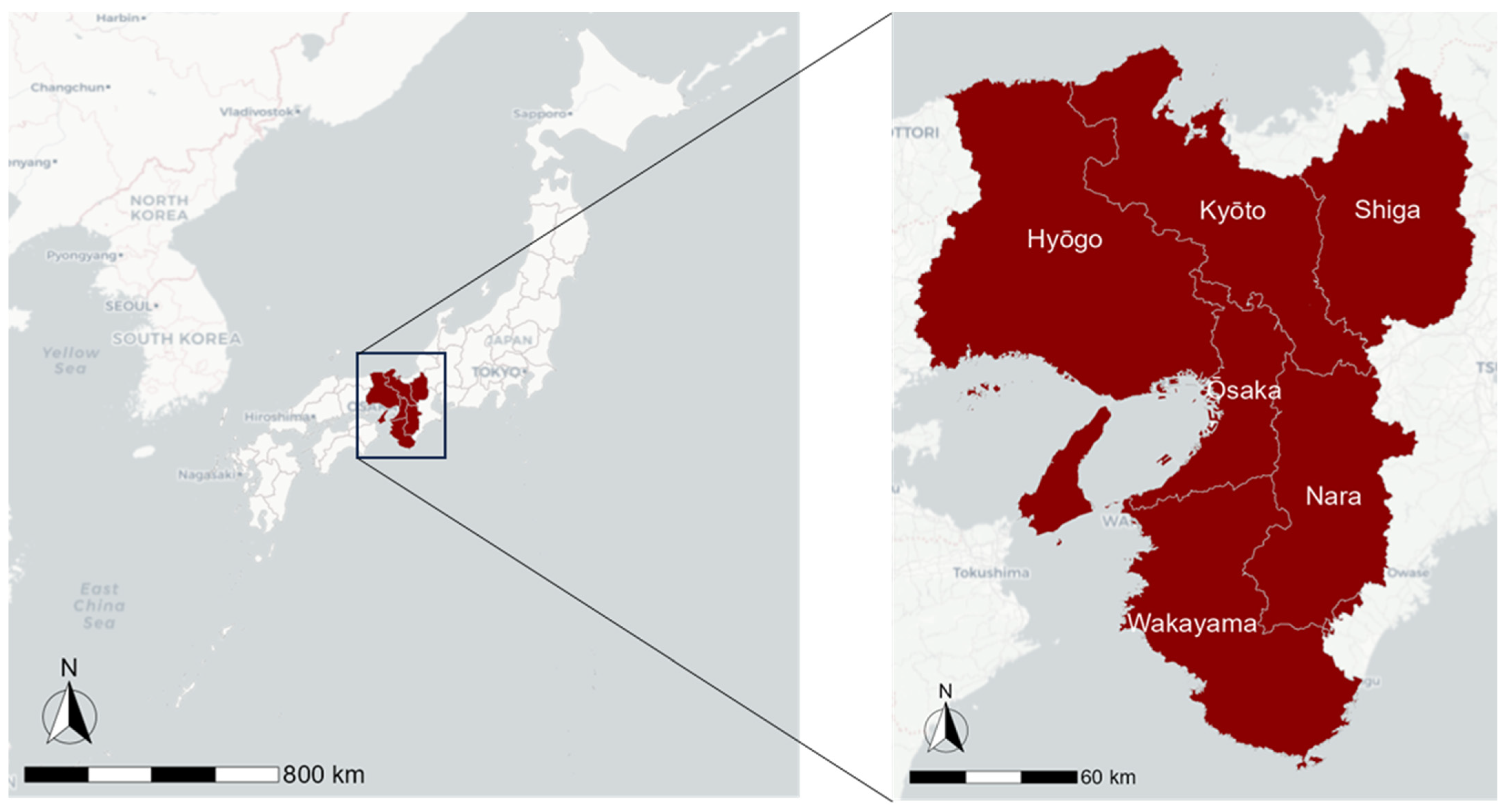
This study focuses on the Kansai region in Japan. The Kansai region comprises six prefectures: Shiga, Kyoto, Osaka, Hyogo, Nara, and Wakayama (see
Figure 1). The population in 2010 was 20.8 million, which decreased to 20.5 million by 2020. It covers an area of approximately 27,000 km
2, with about 70% of the region consisting of forests and mountains. In terms of urban land use, it was 13.1% in 2009, but it increased to 14.0% by 2021. Additionally, there are approximately 7200 km
2 of designated agricultural areas that require comprehensive promotion of agricultural land. However, not all of this land is utilized for agriculture. In 2009, 11.5% of this area was used for urban land, which increased to 13.6% by 2021, indicating a conversion of agricultural land into urban land use.
In this study, we attempt to detect urban sprawl using nighttime light data. Furthermore, to verify the conditions of the detected areas, we utilize land-use mesh data and mesh population statistics.
For the nighttime light data, we use the annual product of the VIIRS nighttime lights (VNL) V2 [
35]. VNL V2 is based on a cloud-free monthly composite generated from the VIIRS-DNB, which provides 12-month mean and median values after solar and moonlight reflections and outliers are removed. The grid size is 15 arc seconds, and it covers the range from 75 degrees north to 65 degrees south. The content of the record is nighttime light radiance, whose unit is nW/cm
2/sr. The VIIRS sensor has been in operation from 2012 to the present, and the annual product of VNL V2 provides yearly data. In the following, nighttime light data are denoted by VNL.
Land-use mesh data were provided by the Ministry of Land, Infrastructure, Transport, and Tourism (MLIT). These data record land-use classifications for each mesh, with a resolution of 3 s in latitude and 4.5 s in longitude. They are created through satellite image interpretation. The data for this study were collected for the years 2009 and 2021. The land-use mesh data are provided irregularly. In this research, urban land use includes classifications such as build-up area, roads, railways, and other developed land uses, which are combined for analysis. The accuracy information of these data is not provided. However, it should be noted that the creation of these data involved 1:25,000 topographic maps and satellite images, meaning they are considered the most accurate land-use data for Japan.
Mesh population statistics are obtained from the national census provided by the Ministry of Internal Affairs and Communications. The mesh population statistics used in this study record residential populations for about 500 m by 500 m meshes, with a resolution of 15 s in latitude and 22.5 s in longitude. The data are collected every five years, and for this research, data from the years 2010 and 2020 are utilized.
Agricultural area data were obtained from the national land numerical information provided by MLIT. The data are from the year 2015 and are provided in polygon format. Subsequent analyses involve converting these data into raster format to match the resolution of each mesh data.
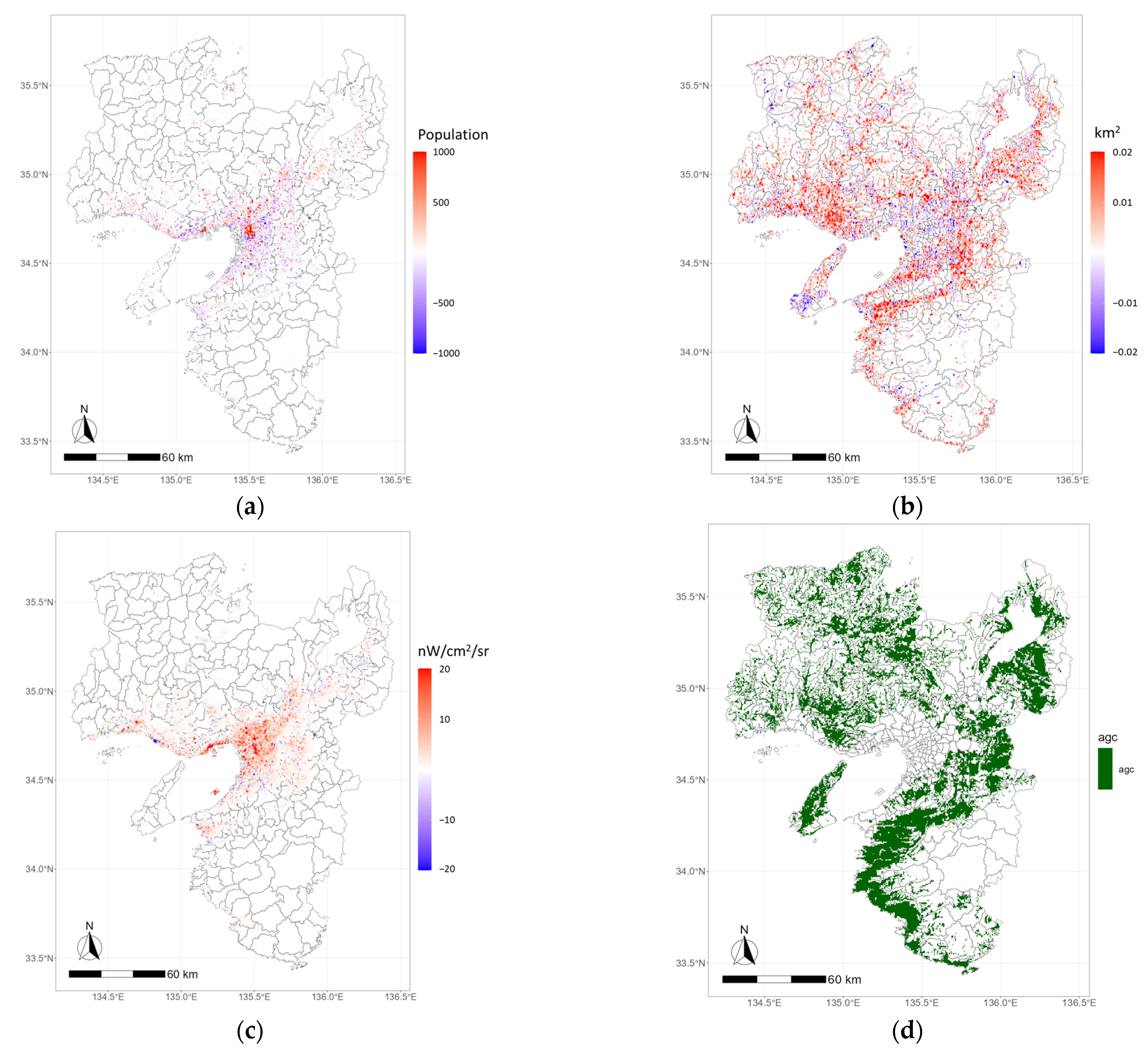
These data for the study area are presented in
Figure 2a, which illustrates population changes from 2010 to 2020, showing significant population growth in urban centers like Osaka, Kobe, Kyoto, and others, as well as a tendency for population growth in some suburban areas. Conversely, there are regions in the near-suburbs of cities where populations are decreasing.
Figure 2b represents land-use changes, aggregated at the 500 m mesh level for clarity. It reveals that while there are some areas where urban land use is decreasing, in many locations, excluding mountainous regions, urban land use is increasing.
Figure 2c displays changes in nighttime lights from 2012 to 2022, indicating increased intensity in many areas, with particularly significant growth in city centers.
Figure 2d represents designated agricultural areas, covering a large region except for urban and mountainous areas.
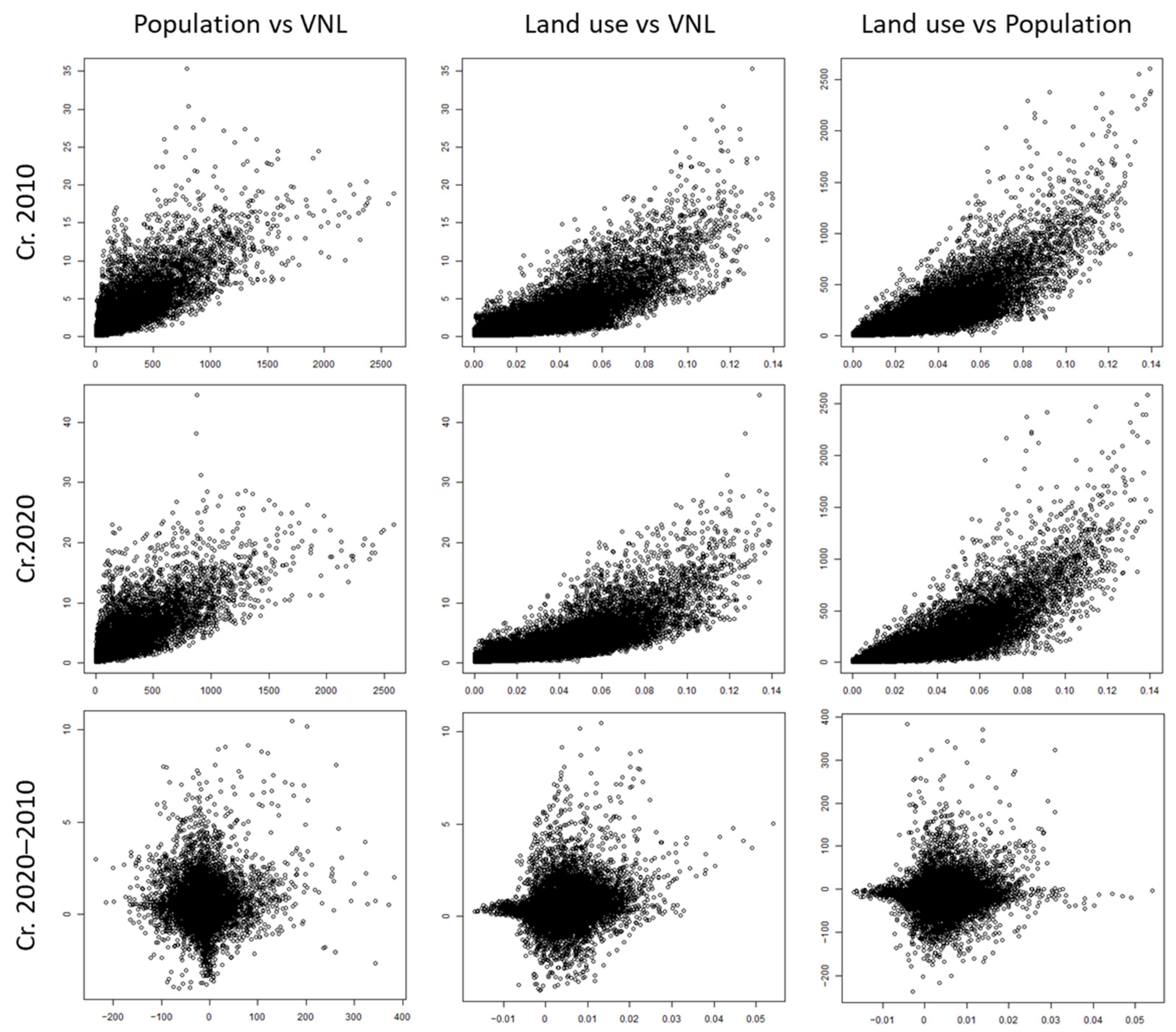
Figure 3 illustrates the correlation of each index in the grids within agricultural areas. These indices utilize data with noise removed by applying a Gaussian smoothing filter, as shown in the workflow of
Figure 4 later. The upper, middle, and lower sections of the figure represent around 2010, around 2020, and the change between 2010 and 2020, respectively. The left side illustrates the relationship between population and nighttime lights, the middle displays the relationship between land use and nighttime lights, and the right side illustrates the relationship between population and land use. Furthermore,
Table 1 presents the corresponding correlation coefficients. It can be inferred that there is a consistent correlation between population, land use, and nighttime lights when viewed in a cross section for each year, all presumed to be associated with urban activities. However, examining the relationship between indices for the change between 2010 and 2020, the correlation coefficients are considerably low. In other words, to detect the progression of sprawl development using this data, there is a suggested need to understand the characteristics of each dataset and combine them appropriately.
Therefore, in this study, we do not consider land-use data as ground truth. Instead, we attempt to extract points with significant changes from the three indicators and verify the characteristics of these locations using aerial photographs. This approach aims to understand the features of each indicator.
2.2. Methods
In this study, we focus on sprawl development within agricultural areas to examine its impact on regional sustainability. For the sake of comparison, all data were converted to a 15 s grid resolution, which corresponds to the VNL resolution, and were used for analysis.
Regarding the land-use grids, we aggregated the urban land use area within each grid. Even within agricultural areas, grids with more than half of their area designated as urban land use at the 2009 baseline were assumed to be urban grids and excluded from the analysis. This resulted in the exclusion of 2% (144 km2) of agricultural grids at the 2010 baseline.
Next, we extracted sprawl points from the changes in population, land use, and nighttime lights. First, for each set of raster data, we applied Gaussian smoothing filters to remove noise and then extracted the top 1% of grids. Subsequently, we detected clumps of extracted grids. Clumps smaller than 5 grids (approximately 1 km
2, assuming extraction of an area larger than the standard neighborhood unit) were excluded, and IDs were assigned based on the sum of raster values within each clump by descending order. This process allowed us to identify areas with significant changes in each indicator. The above workflow is illustrated in
Figure 4.
It is worth noting that the analysis was conducted using R version 4.2.3, and raster data processing utilized the raster_3.6-20 and spatialEco_2.0-1 packages.
3. Results
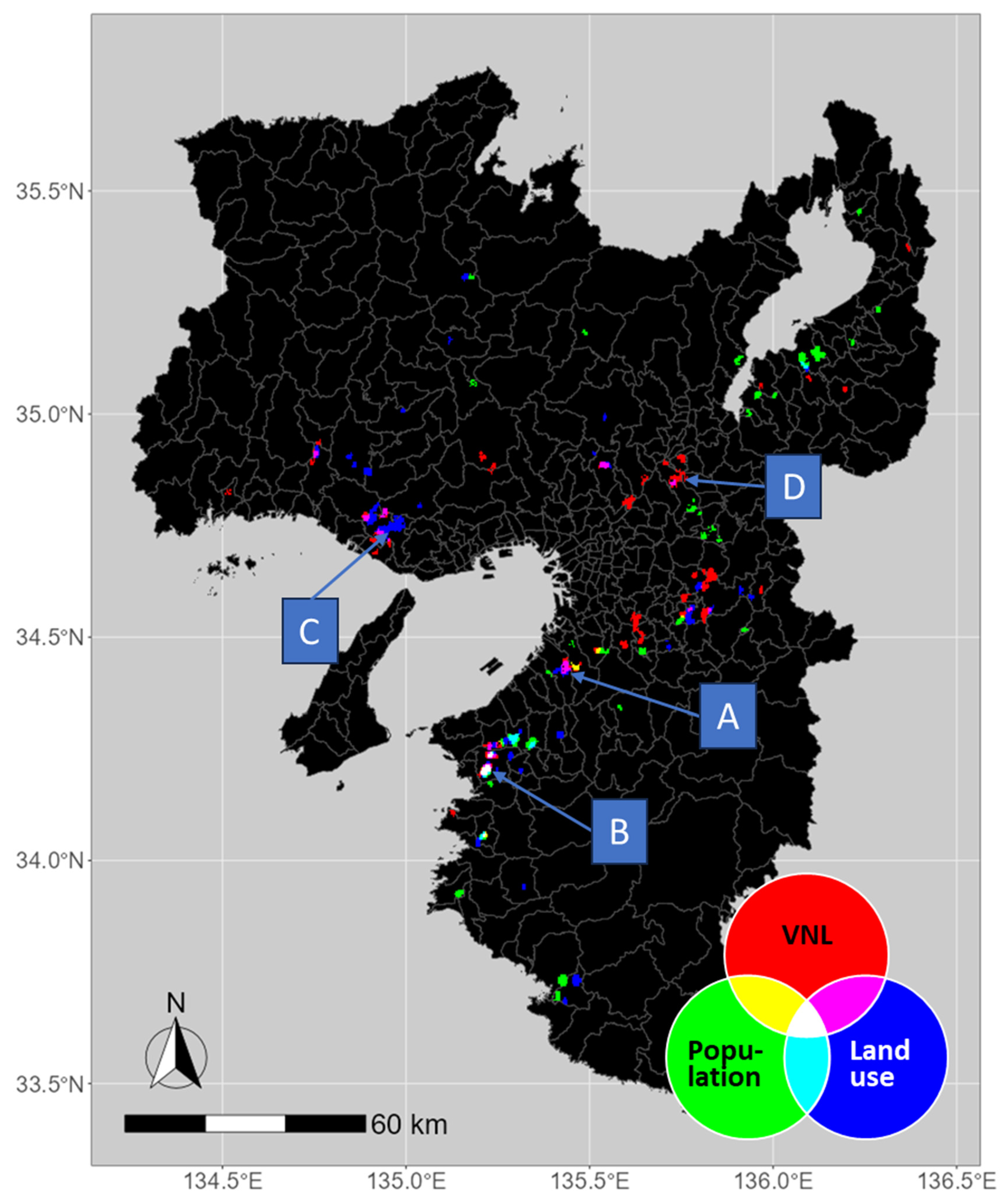
The sprawl areas detected from the population, land-use, and nighttime lights data are presented in
Figure 5. Clumps shown in blue represent areas detected from land use, those in red from nighttime lights, and those in green from population meshes. These locations are represented in RGB color, and grids with overlapping clumps are indicated with the colors in the legend’s Venn diagram. It is worth noting that the number of detected sprawl areas is 34 from land-use data, 36 from nighttime lights, and 33 from population data.
Table 2 shows the aggregated values and areas of the top 10 locations for each indicator among these extracted clumps.
From this, it can be observed that many of the major detected areas are located on the outskirts of urban areas. Among these, this study focuses on four points labeled with letters. “A” is Kishiwada City, Osaka Prefecture, which ranks third in land-use change and VNL change but does not rank within the top 10 in population change. “B” is Wakayama City, Wakayama Prefecture, which ranks fifth in land-use change, seventh in VNL change, and third in population change. Both areas are ranked highly in sprawl intensity across multiple indicators. On the other hand, “C” is Kobe City, Hyogo Prefecture, which ranks first in land-use change but is not ranked in the other indicators. Finally, “D” is Yawata City, Kyoto Prefecture, which ranks first in nighttime lights change but is not ranked within the top 10 in land-use and population change.
The following sections will provide an overview of the situations in these areas.
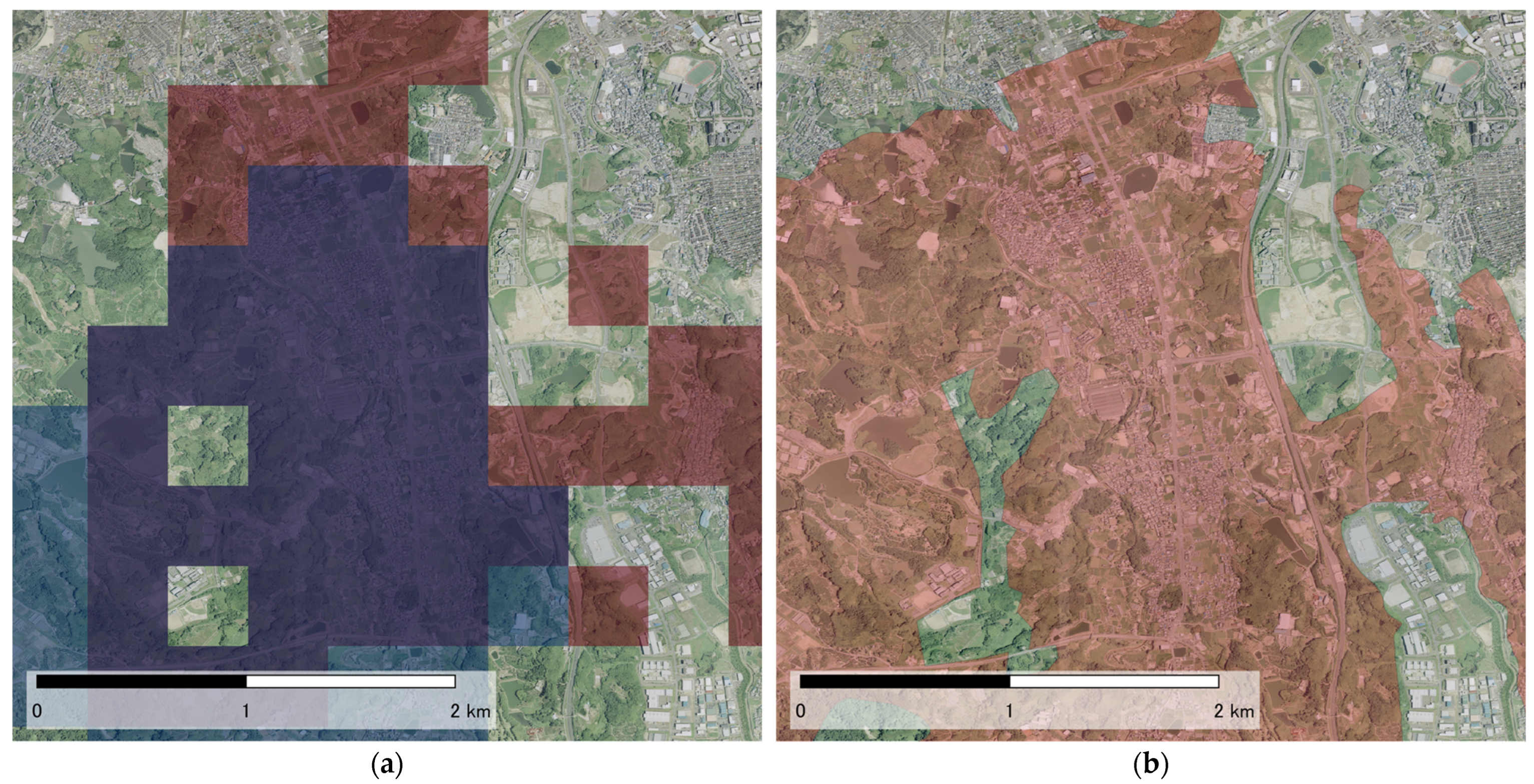
First, the situation at point A is presented in
Figure 6a shows the detected sprawl areas, with blue representing land use, red representing VNL, and green representing grids detected from population data. However, the green grids overlap with all the red grids. Grids where red and blue overlap are indicated in dark blue. On the other hand, green and blue grids do not overlap. At this location, there is a highway interchange within agricultural land, and numerous shopping malls and logistics facilities are located in adjacent non-agricultural land, as shown in
Figure 6b. When comparing the aerial photos from 2007 (
Figure 6c) and 2021 (
Figure 6d), it can be seen that in the agricultural area, forests have been cleared, and large-scale land development has taken place. It is worth noting that even in 2007, significant urbanization had already occurred within the agricultural area. In such areas, development within agricultural land can be captured by the land-use map, nighttime lights, and population mesh used in this study. However, the population data do not capture development for commercial purposes, leading to the detection of points different from the development areas detected from land use.
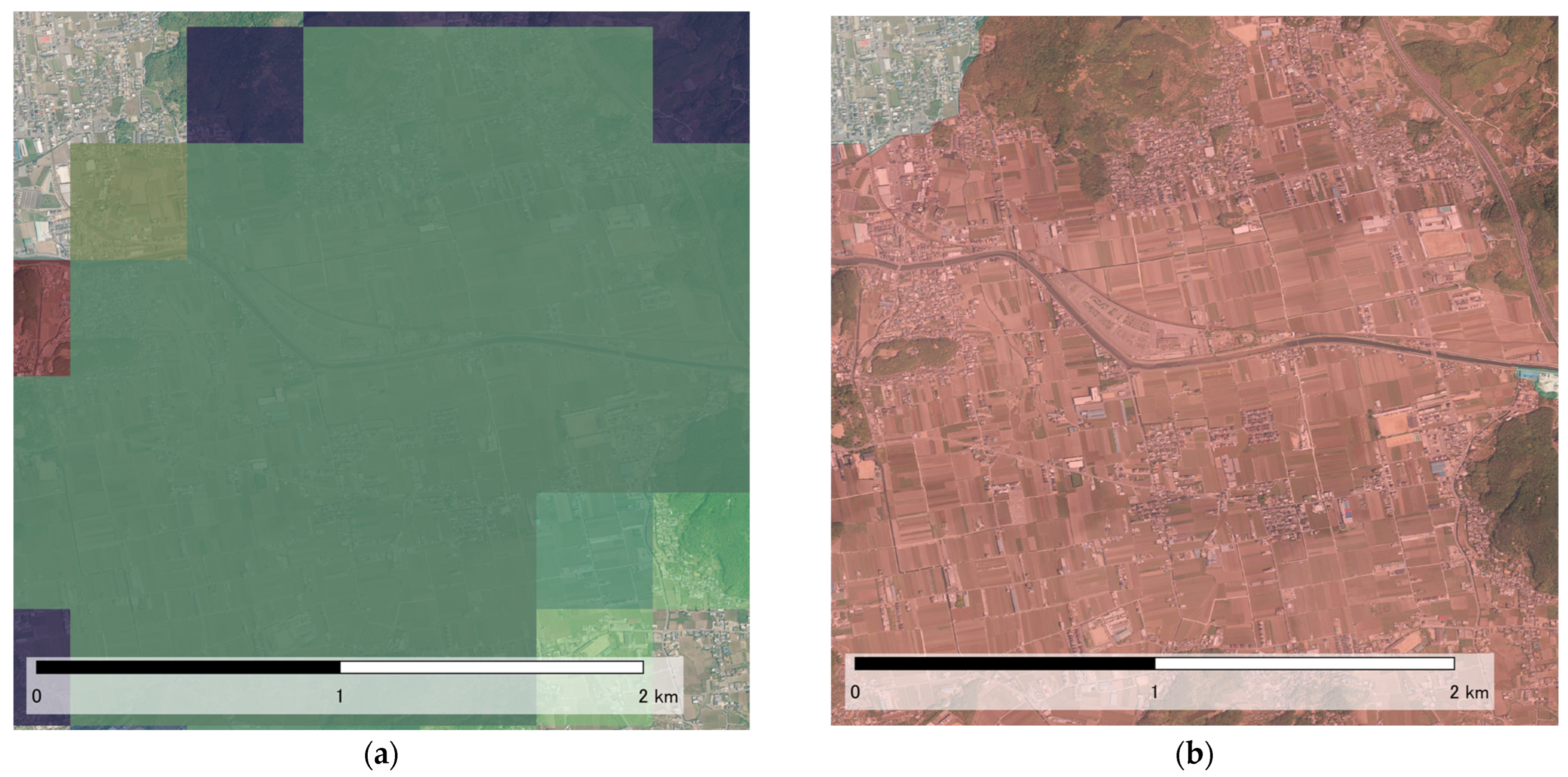
Next, the situation at point B is presented in
Figure 7a, which shows the sprawl areas, similar to
Figure 6, detected from nighttime lights, land use, and population overlap. From aerial photos, it can be seen that residential development has progressed in this area. Additionally, road infrastructure has also been constructed. As a result, sprawl is detected by all indicators.
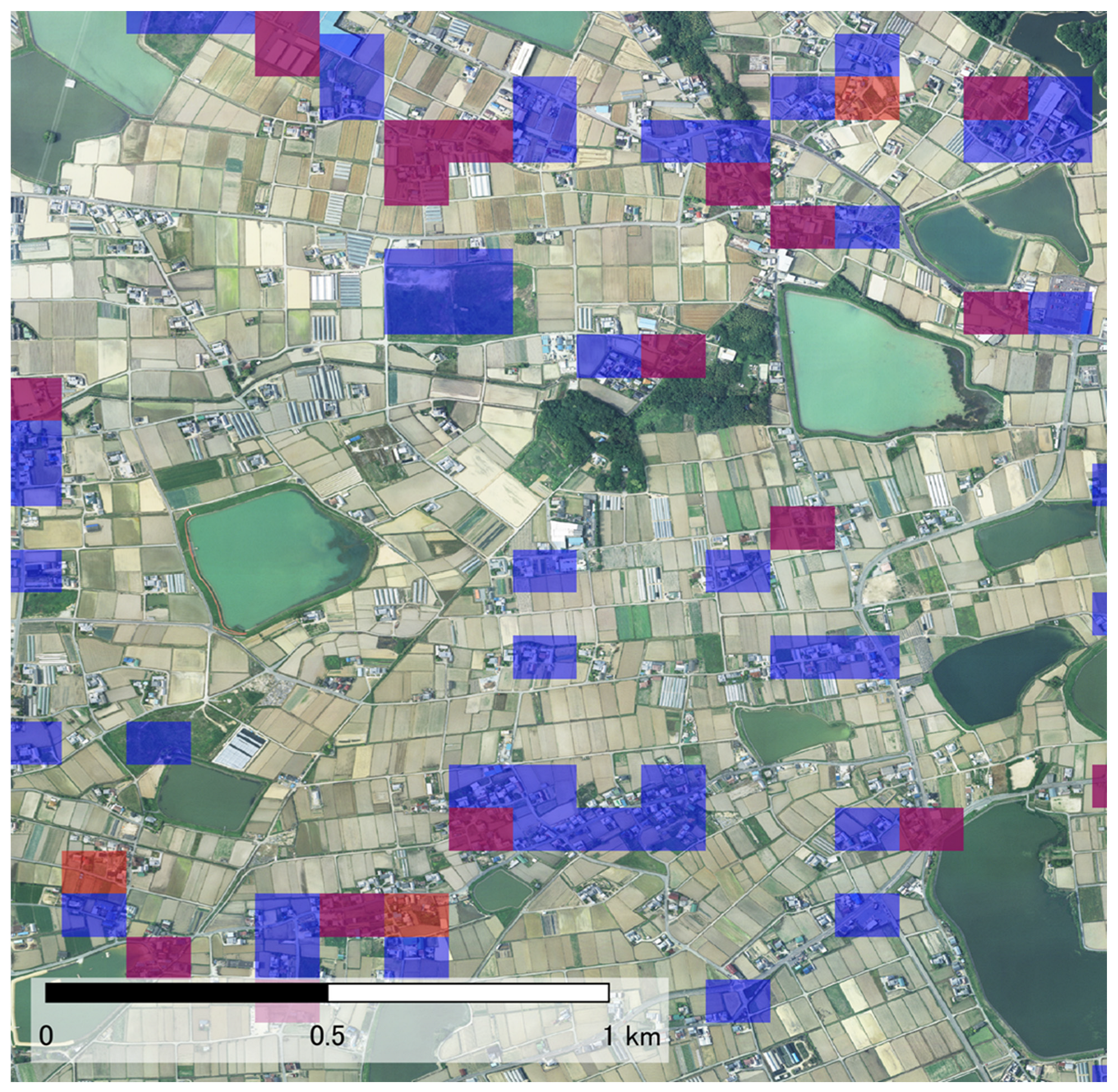
Figure 8 overlays the 2009 aerial photograph of point C with the 2009 and 2021 urban land-use grids in transparent red and blue, respectively. Here, the abundance of blue grids suggests that sprawl occurred in this area according to land-use data. However, upon closer inspection, it becomes evident that in most of the blue grids in 2009, houses are found. Furthermore, it can be inferred that a considerable number of buildings were present even in areas not classified as urban land use. This suggests that in this particular area, sprawl development did not actually progress, but it was estimated as such due to the comparison of data judged under different criteria in different years for classification.
The data source also provides a disclaimer, stating, “The method of land use determination may vary depending on the creation year, therefore users should consider this fact when conducting overlay analysis over multiple years.” This specific area consists of scattered residences within agricultural land, and the small clusters of building plots make satellite image interpretation challenging. To comprehend the development status in such areas, it is likely necessary to reference multiple sources of information.
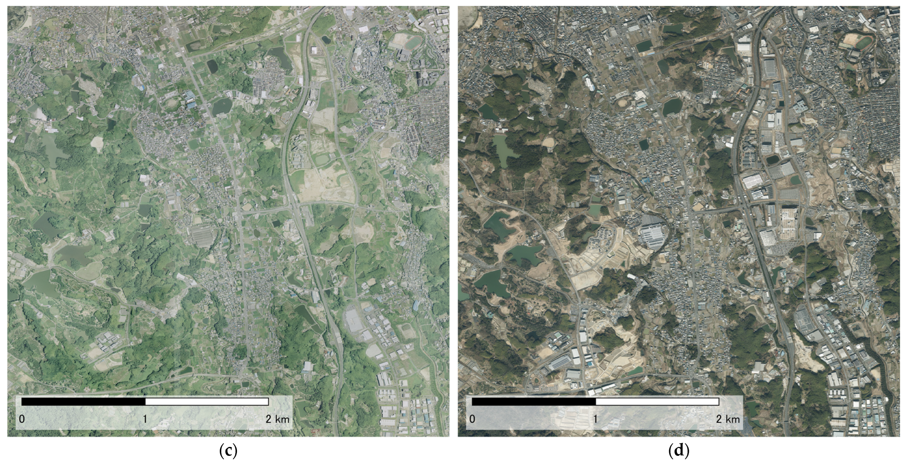
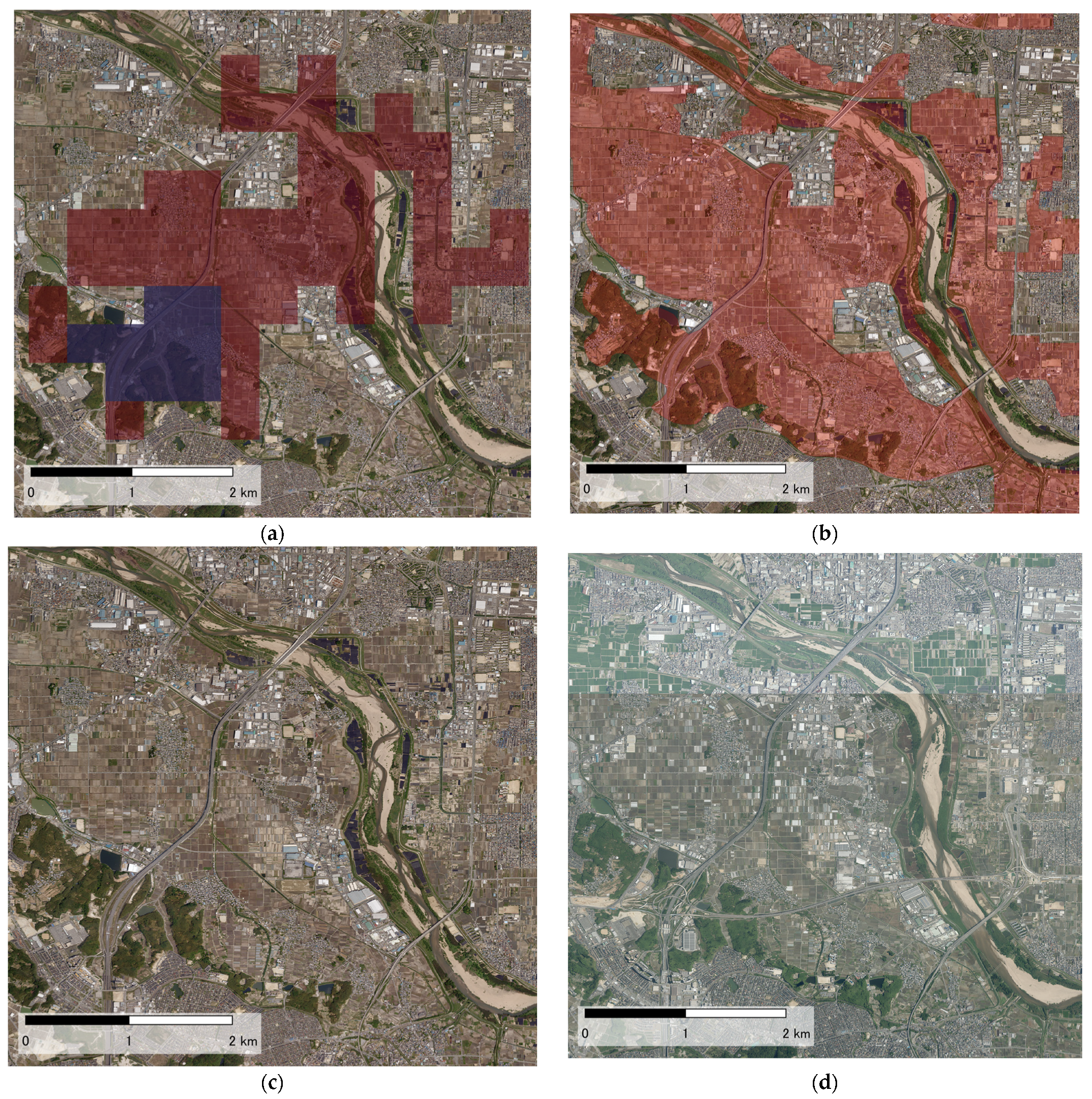
The situation at point D as illustrated in
Figure 9a indicates that sprawl has been determined from nighttime light data across a wide area, although land-use categorization restricts sprawl identification to only a portion of this region. Conversely, population data do not designate this area as sprawl. Examination of land use within the targeted agricultural region using aerial photographs reveals minimal change between 2008 and 2021, with much of the farmland remaining intact, suggesting that sprawl development has not occurred.
The primary divergence in this period pertains to the construction of east–west highways and two interchanges. One of these interchanges is indeed classified as a development site in the land-use dataset. The fact that nighttime light data identify a sprawling area even though land use has not changed substantially can potentially be attributed to an increase in street lighting due to road construction, concomitant with a rise in automobile traffic volume. Consequently, sprawl is detected not only in grids associated with newly established roads and interchanges but also in grids along existing highways. Furthermore, there is a possibility of an increase in areal traffic volume along routes other than the expressways.
It should be noted that the method employed in this study applies Gaussian smoothing for noise reduction, potentially resulting in the classification of surrounding areas of grids with high radiance increases in nighttime light as sprawl development zones. Furthermore, it is worth considering the possibility that the increased use of lighting for purposes such as greenhouse cultivation in agricultural practices to adjust harvesting schedules could lead to an expansion in nighttime light radiance.
4. Discussion
In this study, we attempted to detect sprawl development in designated agricultural areas of the Kansai region during the 2010s using nighttime light data and compared the results with those obtained using land-use and population data. The findings revealed that the regions detected using these indicators do not always overlap perfectly, and different areas are detected based on the characteristics of each dataset. The results indicate that despite population decline, there are many areas that should be preserved as agricultural land but are experiencing sprawl development.
Sprawl development is fundamentally understood as the transition from natural land use to urban land use. However, spatial data regarding land use based on registration information are limited, necessitating reliance on satellite imagery and similar sources for broad-scale assessments. Nevertheless, our study highlights the potential for misjudging land-use changes when comparing datasets with differing classification criteria. Therefore, it can be argued that detecting sprawl requires the comparison of multiple sources of information.
Nighttime light data directly measure the intensity of light and do not directly quantify land-use changes. However, in many contemporary urban areas, light is emitted from streetlights and buildings, making nighttime light data a potential surrogate indicator for urban development. It is important to note, though, that changes in the amount of light emitted at night do not necessarily correspond solely to urban development. They can also result from increased automobile traffic or the addition of lighting to existing facilities, among other factors. In such cases, detection may occur even when sprawl development is not occurring.
For instance, in the case of Location D in
Section 3, it is possible that increased traffic due to the construction of highways and interchanges is being captured. However, this may be indicative of improved regional accessibility and increased activity levels, which could be interpreted as an increase in the area’s utility and the potential for future urban development. Such areas may warrant closer attention in terms of controlling sprawl development.
From the mesh population data, population increases due to residential development can be captured, but they cannot supplement developments for commercial purposes. Moreover, instances where buildings become taller may result in population increases without necessarily involving land-use conversion. Therefore, spatial population data are considered insufficient as an indicator to capture sprawl development.
Furthermore, the frequency of data maintenance varies depending on the data source. In the case of land-use mesh data in Japan, they are updated at irregular intervals, with data provided for 2009, 2014, 2016, and 2021. While specific details about the interpretation method are not disclosed, it is known to make use of image products like SPOT and RapidEye. Satellite imagery usually requires adjustments for interpretation due to variations in observation times and conditions, and it is generally not fully automated. Therefore, data maintenance is presumed to incur significant costs, and regular updates are not conducted in Japan.
Mesh population data in Japan are updated every five years based on the national census. However, few countries regularly publish such spatial population statistics. On the other hand, nighttime light data provide composite images on a monthly basis, and annual average composite images are available based on the median of cloud-free nighttime light radiance. Consequently, nighttime light data offer features with a higher frequency compared to land-use and population mesh data. However, it is important to exercise caution when comparing monthly images in regions with snowfall, as snow cover can affect radiance levels, causing them to be higher during the winter months.
Land-use mesh data are secondary data obtained through classification processing based on satellite imagery, while population mesh data are created based on statistical surveys. Consequently, the maintenance status of these data varies from country to country. The European Space Agency Climate Change Initiative Land Cover data (
https://www.esa-landcover-cci.org/, accessed on 19 November 2023) provide annual global land cover data from 1992 to 2020. However, the spatial resolution is 10 s. In this study, we used data with a higher spatial resolution. Still, such data may be useful when targeting countries where detailed land cover data is not available.
On the other hand, nighttime light data target nearly all terrestrial areas inhabited by humans and are accessible for use worldwide. The summarized characteristics are presented in
Table 3.
In a previous study, [
47], the authors attempted to detect sprawl using population grid data with K-means clustering and local spatial entropy. They estimated sprawl areas straightforwardly from population data, considering it a convenient method. However, this study defined sprawl exploratively based on population and its grid arrangement, requiring empirical judgment to identify sprawl areas. Additionally, it did not compare with other indicators such as land use.
The authors of [
48] defined the degree of sprawl based on the entropy index using the ratio of build-up areas. They calculated the extent of sprawl in urban areas based on this index. Land-use data in this study were estimated using Landsat satellite images with 150 ground truth data and adjusted to reproduce ground data using field knowledge. Consequently, considerable effort was invested in data creation.
The authors of [
40] estimated urban spatial changes using DMSP-OLS nighttime light images, validating it by comparison to detected build-up areas from Landsat TM images used as ground truth. The discernment accuracy of urban pixels was reported to be just under 70% in terms of the geometric mean measure. However, this evaluation was a cross-sectional accuracy assessment, and the reproducibility of changes in urban areas was not assessed.
In this study, we confirmed the relationships between changes in each indicator. While there is high correlation between indicators when viewed cross-sectionally, we found very low correlation regarding changes. This suggests that these indicators can be utilized as independent measures to capture changes in urban areas, providing a novel insight in this study.
In summary, it can be said that nighttime light data are useful for complementarily understanding sprawl, even when time-series land-use data and spatial population data are available. Furthermore, in areas where land-use data and spatial population data are not available, the nighttime light data can be useful for capturing spatial changes in urban activities. The method used in this study is simple, and the computational requirements are minimal, making it easily applicable.
However, in this study, we only extracted and verified locations with significant changes in nighttime light and other indicators. For each of these indicators, we extracted the top 1% of grids and further selected the top 10 locations within those clumps. We then verified the land use conditions based on aerial photographs, especially for locations with particularly significant changes. Therefore, the insights presented in
Table 3 are specific to the study area, and it should be noted that different characteristics may be observed in other regions.
In the future, it is necessary to investigate whether land-use changes can be observed even in locations where lower-level changes are detected, and research on the lower limits of sprawl detection is required. When detecting fixed or steady sources, it may also be useful to examine the temporal stability of nighttime light intensity. The VNL data targeted in this study are consistently observed, organized, and publicly available, allowing for verification of temporal stability. Furthermore, in this study, Gaussian smoothing was used for noise reduction and area identification. However, this can introduce bias in estimates around grids with high nighttime light intensity. Therefore, it is necessary to consider the application of more sophisticated methods, such as topological data analysis of point sets in clump detection.
This study focused on extracting areas with a high likelihood of sprawl in agricultural land. Despite a decrease in the overall population in the region, it was estimated that there is still a considerable possibility of sprawl development in many areas. As seen in
Figure 2, the continued new urban development on the fringes of the city, even though there are other areas where infrastructure is already in place and the population is decreasing, could potentially reduce the population density of the region and decrease the efficiency of the city in terms of increased travel distances and decreased efficiency of urban activities. In addition, residential development in agricultural areas may lead to decreased agricultural productivity, disruption of ecosystems, and environmental degradation, as discussed in previous studies [
7,
12,
13,
15,
21,
49].
If such sprawl development continues, it could lead to a decline in the sustainability of the region. To control this, monitoring of local spot development situations alone may not be sufficient, and observation on a regional scale is required. In this regard, the wide-area detection method proposed in this study could be effective.


