Development and Analysis of Optimization Algorithm for Demand-Side Management Considering Optimal Generation Scheduling and Power Flow in Grid-Connected AC/DC Microgrid

Abstract

The world energy sector is experiencing many challenges, such as maintaining a demand–supply balance with continuous increases in demand, reliability issues, and environmental concerns. Distributed energy resources (DERs) that use renewable energy sources (RESs) have become more prevalent due to environmental challenges and the depletion of fossil fuel reserves. An increased penetration of RESs in a microgrid system facilitates the establishment of a local independent system. However, these systems, due to the uncertainties of RESs, still encounter major issues, like increased operating costs or operating constraint violations, optimal power management, etc. To solve these issues, this paper proposes a stochastic programming model to minimize the total operating cost and emissions and improve the operational reliability with the help of a generalized normal distribution optimization (GNDO). A day-ahead demand response is scheduled, aiming to shift loads to enhance RES utilization efficiency. Demand-side management (DSM) with RESs is utilized, and battery energy storage systems in low-voltage and medium-voltage microgrids are shown. Mathematical formulations of each element in the microgrids were performed. Optimal and consumer-friendly solutions were found for all the cases. Environmental concerns based on the amount of harmful emissions were also analyzed. The importance of demand response is demonstrated vividly. The aim is to optimize energy consumption and achieve optimum cost of operation via DSM, considering several security constraints. A comparative analysis of operating costs, emission values, and the voltage deviation was carried out to prove and justify their potential to solve the optimal scheduling and power flow problem in AC/DC microgrids.

1. Introduction

Demand-side management (DSM) represents a set of widely used strategies for satisfying the electricity demand of consumers such that their cost of energy consumption is minimized. The demand of the consumers under a DSM can be scheduled given time-varying electricity prices (e.g., day-ahead market prices). This DSM approach will be referred to as a demand response (DR) program. Alternatively, the demand of the consumers under a DSM can be satisfied by combining the power bought from the grid and the power locally produced/stored by the consumers [1]. This DSM approach will be referred to as a renewable energy sources (RESs) deployment problem. In this paper, we develop and analyze novel DSM strategies for residential and industrial owners.

In recent years, the issue of minimizing the cost of energy consumption for electricity consumers has emerged as an important research topic. The strategies for reducing the energy consumption cost for consumers can be broadly classified as demand response (DR) programs and the deployment of renewable energy sources (RESs). These strategies can be collectively referred to as demand-side management (DSM) [2].

The present paper concentrates on the usage of DSM in various aspects, viz., in residential, commercial, and industrial areas of low- and medium-voltage MGs. The impact of DR is evaluated under different conditions. The intelligent charging of BESSs is also shown. An environmentally friendly and customer-comfort-centric analysis is presented. All these evaluations were carried out using appropriate optimization algorithms, and the capability of the algorithms has been validated.

1.1. Literature Review

Microgrid analysis is mainly focused on control and energy management strategies, both in the islanding and grid-connected modes. The study also includes the integration of generators, renewables, storage systems, and various loads, along with their uncertainties and design modeling [2]. Energy management includes the optimal dispatch of energy, scheduling, modeling, and their solving methods [3]. Meanwhile, the control problem includes the voltage, frequency, and power as crucial variables [4]. In some cases, the impact of the unique components of the grid is also investigated. In particular, for sustainable microgrid implementation, the influence of BESSs was reviewed in a cost-effective and efficient way. Also, various uncertainties have been considered, along with their analytical and approximation techniques to observe the renewables’ impact on system control and monitoring [5]. Thus, it has been observed that the development of the microgrid is primarily influenced by the energy DSM, renewable energy penetration, and its integration into the utility grid. In [6], a standalone microgrid was developed economically with renewable and energy storage systems for remote communities. However, the islanding system’s development issues and challenges were analyzed in regard to the utility power grid [7], whereas with residential loads, a demand response strategy was implemented with a grid-connected microgrid [8]. The inclusion of renewable energy sources (RESs), BESSs, demand-side management (DSM), and SPVs are addressed with economic assessment in these initiatives.

DSM is a powerful tool to facilitate the process of transforming traditional microgrids (MGs) into green systems [9]. MGs, which are self-sufficient energy systems that serve a small geographical area’s energy needs, are generally discussed in association with renewable energy sources (RESs). DSM with MGs allows the grid managers to observe the difference in the performance of conventional MGs to those powered by renewable energy. It helps with the instability of RESs. DSM allows the grid managers to observe and carry out the efficient utilization of RESs and an economic consumption of power by the consumers. The inclusion of RESs helps in meeting growing power demand and reducing emissions, which eventually make the system sustainable and environmentally friendly, respectively. DSM promotes generation through distributed energy resources (DERs), as it facilitates the avoidance of long-distance transport. Locally generated energy may be consumed by local loads, immediately. DERs majorly include RESs, battery energy storage systems (BESSs), and controllable loads, which benefit both electricity consumers and the electric utility if the integration is properly engineered. BESSs help mitigate the volatility of RESs and reduce additional stress on the grid. Industrial experts refer to DSM-coupled BESSs as the bare bones of smart grids. Time-of-use pricing with storage helps in flattening the load curve, while the strategic installation of BESSs saves significant costs for operators [10,11].

The deployment of AC/DC microgrids has become an emerging area of research. Energy trading with locally generated power by consumers has been discussed in the literature [12]. There has been tremendous support for the installation of PV units and BESS units in several countries [13,14]. This helps consumers reduce their cost of energy consumption. Residential consumers have opportunities to share their common rooftop areas to install solar units and BESSs. Many works in the literature have focused on the problem of energy trading (including demand scheduling) using PV generation (e.g., [15,16]). In these works, it was assumed that PV generation was available. In other words, PV units were pre-installed at the consumer premises. The objective of energy sharing is to minimize the cost incurred for buying power minus the revenue from selling locally generated/stored power (referred to as the net cost) over an operating day. However, it is important to find the optimal number of PV units and BESS units to be installed in order to satisfy the energy requirements of the consumers and achieve annual cost savings for the consumers. In other words, the real advantages of energy trading by the consumer will be realizable only when the investment problem and the energy trading problem are jointly considered. Hence, the combination of microgrid investments and energy-sharing options becomes an important research topic. In recent years, few works have dealt with investments in PV generation or BESSs for reducing the expected energy consumption costs incurred during the investment period. The majority of the works have considered a single consumer’s investment problem (e.g., building owner [17], microgrid operator [18]). Very few works have considered the shared investment model combined with the energy trading problem for multiple consumers based on only BS units [18,19].

A two-stage SMIP for determining the optimal capacities of the energy storage system and fuel-based generation for an islanded microgrid was proposed in [19]. The operational cost under different random scenarios was minimized based on the year of installation of the BESS. Owing to binary variables in both stages, a new decomposition method was developed for finding a sub-optimal solution. A two-stage stochastic program was proposed to design an energy hub consisting of energy storage, photovoltaic power, combined heat and power generator, and various heat and electricity loads in [20]. In [21], a microgrid operator determined the optimal capacities of renewable energy resources such as solar power and wind power, and capacity of energy storage based on the predicted values of the meteorological data. A two-period stochastic linear problem was proposed for this purpose in [21]. In the first period, the investment decisions were found, whereas in the second period, supply demand matching within the microgrid was performed. The operator bought power from the grid whenever the harvested energy plus stored energy was insufficient in real-time. Online DSM has been utilized in [22] to study the effects of uncertainties in MG for DSM. A framework has been developed in [23] to control and optimize an MG with a photovoltaic (PV) system, load, electrical vehicle (EV) charging stations, and a storage unit while using model predictive control. For a non-deferrable load facility with the ability to harvest and store renewable energy, a demand management strategy was suggested in [24]. In [25] have proposed a two-stage price-based DR strategy for the coordination of DG. The model has been framed considering hourly operation, customer bills, and demand energy quantity and voltage regulation to maximize customer benefits.

A DSM framework has been designed in [26] that acknowledges the interconnection of smart users, non-controllable loads, energy, and comfort-based controllable loads, and individual PEVs. In [27], the authors have modelled hybrid MG by utilizing the concept that each home has to be equipped with more solar PVs than are required for normal operation. In [28], the authors have introduced a DSM model specifically for rural areas. Renewable energy’s inherent stochastic behavior and the difficulty in predicting electric load have been tackled in [29] for the proposed DSM modelling. In [30], the authors have analyzed different of DSM approaches to shift the AC devices optimally in the presence of DC MG. In [31], the authors have proposed a feeble power handling scheme in hybrid MG where AC and DC loads have been bifurcated and are supplied by utility and PV along with a battery, respectively. Optimization algorithms provide a large premise for solving several engineering problems. In [32], the authors used PSO for energy scheduling of the IEEE 14-bus system in the form of virtual power plant which constitutes RESs integrated MGs. In [33], compared several optimization algorithms such as binary PSO, wind-driven optimization, GA, ant colony optimization, and bacterial foraging algorithm while analyzing energy management systems for residential areas. In [34], the authors used a hybrid of GA, PSO, and wind-driven optimization algorithms to design appliance schedulers and energy management controllers. Robust optimization methods proposed in [35,36,37,38,39,40] to solve practical engineering problems consider uncertainties.

1.2. Research Gap and Scope

DSM (demand-side management) in a microgrid is considered for both the utility side as well as the consumer’s side. Along with DSM, BESS is reviewed with renewable energy sources in the literature. SPV and BESS application to home energy management as both load and source are considered. In this paper, DSM is also considered along with renewable energies in a microgrid environment. The major shortcomings are as follows; (i) Microgrid energy management is much more focused on supply-side management. So, operational constraints such as voltage and losses are taken as the primary objective. The load control is to be performed from the utility side; (ii) Pricing schemes designed for system control rather than customer feedback interpretation; (iii) BESS are mostly categorized in home loads, and the charging scenario is considered. BESSs are to be analyzed in a microgrid environment; (iv) Simultaneous coordination between RESs and BESSs is missing. The impact of one on another is not addressed yet; (v) Many researchers are focused on the one-way direction optimization of solar PV. PV can be addressed to mitigate the effect of BESS injection. However, the reverse is not quantified; (vi) Home load energy management is only focused on consumption pattern. A gap is established between home and grid interaction.

The following scope of research has been framed as objectives of the research work: (i) A bidirectional mode of operation is established for DSM. The demand response is designed for valley filling and peak clipping methods. BESS with solar PV is used to fulfil the above scenarios for maintaining the flat demand profile. The effect of SPVs inclusion conditions along with the BESSs is considered simultaneously in load management. (ii) Primarily, the impression of RESs integrations into the microgrid system is analyzed with proper BESS load modeling in order to incorporate the research objective. The SPVs and BESSs are considered, and their impact on the grid is analyzed with different levels of penetration. The integration is also characterized by its position in the grid. The use of photo-voltaic power generation is also coordinated to integrate BESSs that retain the stability of the system with a minimum incurred cost. (iii) A metaheuristic search approach has been adopted for DSM setup to schedule smart appliances with minimum energy bills by utilizing the bidirectional energy flow of BESS. This study mainly includes two issues: (a) a framework is proposed in a decentralized manner to schedule the loads using DSM, and (ii) the population-based optimization algorithm is applied to find optimized perdurance. The method with a reduced bill for the customer along with their comfort and BESS integration in a microgrid is also implemented in this case.

1.3. Contributions

The futuristic needs of MGs and their demand management have inspired the author to explore opportunities for potential consumers. The motivation behind the proposed work is to analyze the operation of an interconnected AC/DC microgrid when DGs are connected to it, and when DR is applied to the same, DR helps in covering up the uncertainties of PV. The motive is to provide a cost-effective solution to the consumers through the usage of the generalized normal distribution optimization (GNDO) algorithm. The GNDO algorithm has been chosen as it is robust, simpler to implement and does not require any specific tuning parameters, unlike contemporary algorithms. The prime contribution of the paper is to introduce an intelligent solution for the DSM problem for different modes of MGs through metaheuristic optimization techniques. The specific contributions of the present research work are as follows:

• This paper provides the complete scheduling of the grid-connected AC/DC microgrid. The response has been evaluated after imposing DR on the system. This is to assess the potential of the generalized normal distribution optimization (GNDO) algorithm in the process of determining the optimal operating cost of AC/DC MG. The GNDO has been used for the first time for the chosen power system-related optimization problem, as it is the most recent optimization algorithm and does not require any tuning parameter. A comparative hourly cost analysis has been conducted for the test system between contemporary algorithms and GNDO. Generation and load demand balance and active power constraints have been maintained for the AC/DC MG test system. A reduction in the amount of CO₂, SO₂, and NOx emissions has been presented.
• Unlike the existing works, the proposed shared RES investment problem deals with the sharing of PV units. Further, the proposed shared investment problem also deals with the sharing of BESS units. The proposed problem optimally determines the virtual share of every residential consumer in the co-owned BESS units and PV units.
• This paper demonstrates a day-ahead DSM through the use of the load shifting technique and presents the novel GNDO algorithm, as an efficient tool for optimizing cost in the context of demand management on SG framework. The efficacy of the proposed GNDO algorithm is demonstrated in comparison to contemporaries for the present application.

The framework of this paper is carried forward as follows: grid-connected AC/DC microgrid is presents in Section 2; modelling of DSM is reported in Section 3; the formulation of problems with security constraints are presented in Section 4 with a subsection for the different cost model of power–generating units, the renewable uncertainties cost model of solar, and BESS; the objective functions and several types of security constraints for the proposed model are reported in Section 4; the optimization algorithm GNDO and its implementation process is described in Section 5; the simulation results of study systems with different cases and findings are discussed in Section 6; and finally, concluding remarks are presented in Section 7.

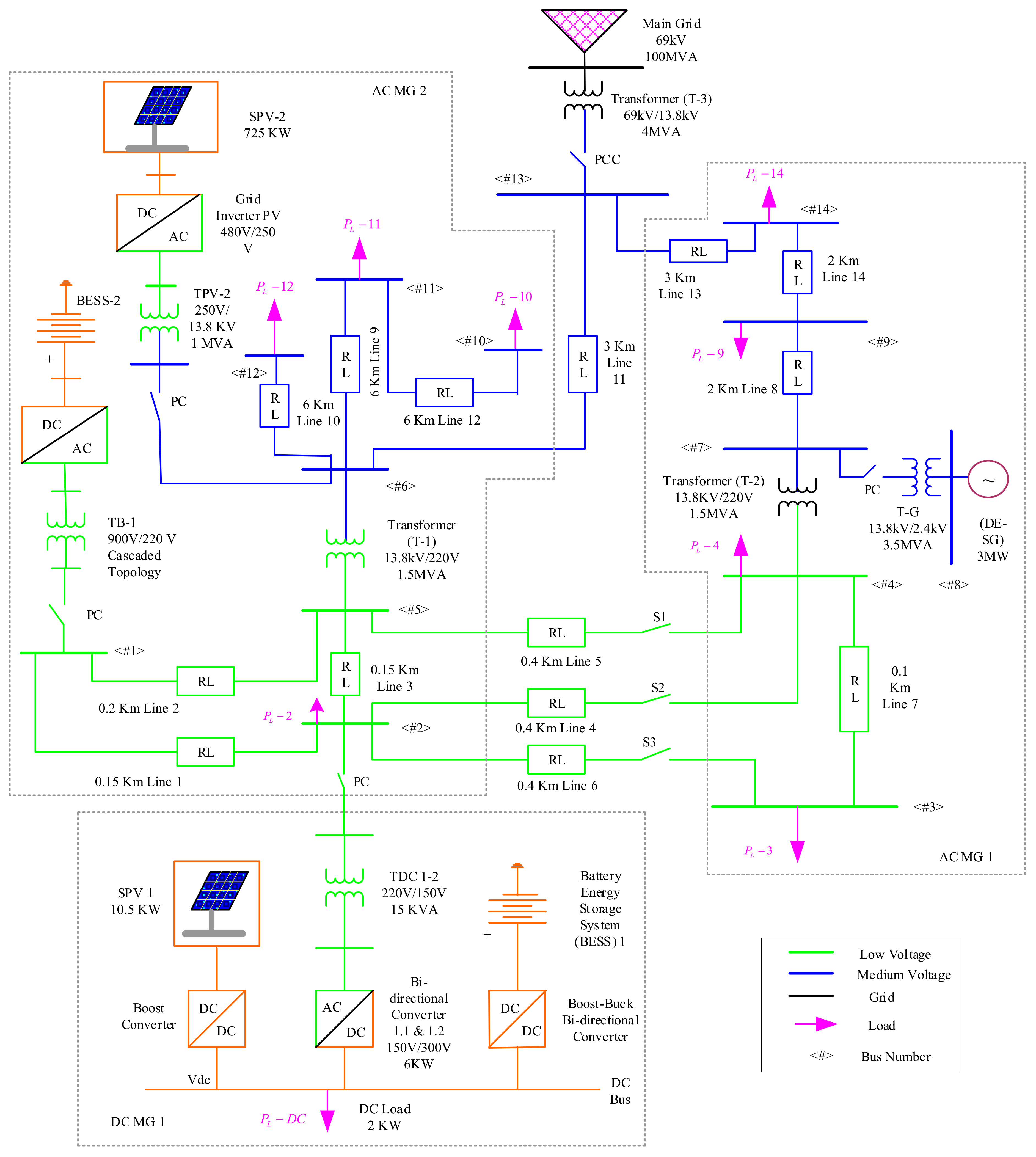
2. AC/DC Microgrid System

The AC/DC MG system shown in Figure 1 consists of two AC and one DC interconnected microgrids and is connected to a 69 KV grid sub-system through PCC, which is similar to the IEEE 14-bus distribution system. The first AC microgrid (AC MG 1) consists of a 3 MW diesel generator (DE-SG) which is coupled through 13.8 KV/2.4 KV, 3.5 MVA transformer to the system. The second AC microgrid (AC MG 2) consists of a 725 KW solar system (SPV-2) and a battery energy storage system1 (BESS-2). SPV-2 is coupled through a 480 V/250 V grid converter and 250 VV/13.8 KV, 1 MVA transformer to the system. BESS-2 (3 nickel-metal-hydride, 650 V) is connected through a bi-directional converter and a 900 VV/220 V transformer to the system. The DC microgrid (DC MG) consists of a 10.5 KW solar system (SPV-1) and a battery energy storage system1 (BESS-1). SPV-1 is coupled through a 150 V/300 V grid converter and 220 VV/1150 V, 15 KVA transformer to the system. BESS-1 (lithium-ion battery, 120 V) is connected through a bi-directional converter to the system. The operational frequency of the system is 60 Hz. The whole system consists of 7 transformers, 14 power lines, 14 AC buses (some buses are low voltage, and some buses are medium voltage, as shown in Figure 1), and 1 DC bus. The AC/DC MG is designed according to [41,42,43]. The line data and load data are given in

Table 1. Line data of AC/DC microgrid.

Line No.	$\mathit{R}\left(\mathit{\Omega }\right)$	$\mathit{X}\left(\mathit{\Omega }\right)$	Length (km)
@1	0.0297	0.016335	0.15
@2	0.0396	0.02178	0.2
@3	0.0297	0.016335	0.15
@4	0.0792	0.04356	0.4
@5	0.0792	0.04356	0.4
@6	0.0792	0.04356	0.4
@7	0.0198	0.01089	0.1
@8	0.788	0.2336	2
@9	2.364	0.7008	6
@10	2.364	0.7008	6
@11	1.182	0.3504	3
@12	2.364	0.7008	6
@13	1.182	0.3504	3
@14	0.788	0.2336	2

and

Table 2. Load data of AC/DC microgrid [35].

Bus No.	Load	High Load (kVA)	Low Load (kVA)	Power Factor
<#2>	$P_L-2$	40	12	0.9
<#3>	$P_L-3$	30	9	0.85
<#4>	$P_L-4$	50	15	0.9
<#10>	$P_L-10$	320	96	1
<#11>	$P_L-11$	800	240	0.8
<#12>	$P_L-12$	400	120	0.8
<#13>	$P_L-13$	800	240	0.8
<#15>	$P_L-15$	1600	480	0.8
<DC>	$P_L-DC$	2	0.6	0.9

, respectively.

2.1. Battery Energy Storage System

It is difficult for renewable energy to meet the consistent load demand because its output reacts slowly and has a limited duration and availability. By adding a storage device, a hybrid energy system can become more efficient and capable. In an AC/DC microgrid system, excess power produced by the systems is stored in the battery, which can be used when the systems are not producing energy. When an MG system’s power generation is insufficient, battery energy is used to support energy consumption.

In the case of renewable energy, the charging phenomena of the batteries require more energy generation than the daily energy requirement. For this study, nickel metal hydride (NMH) and lithium-ion batteries were selected since they are well known for their suitability for storage of renewable energy resources. Their battery storage has a voltage rating of 650V and 120V DC and a capacity rating of 1.5 and 800 Ah. Depending on the type of battery storage, their rated efficiency values are between 20% and 80% [44]. The BESS data are given in

Table 3. BESS data.

Unit	No. of Battery	Initial SOC (%)	Rated Capacity (Ah)	Nominal Voltage (V)
BESS-1	1	80	800	120
BESS-2	3	80	1.5	650

. The charging and discharging operation of the NMH and Li-IO batteries can be represented [45] as follows

$$E_{C,NMH}=E_0-p\left(\frac{Q}{\left|Q^{*}\right|-0.1Q}\right)\widehat{i}-p\left(\frac{Q}{Q-Q^{*}}\right)Q^{*}+e^t;\widehat{i}<0$$

(1)

$$E_{DC,NMH}=E_0-p\left(\frac{Q}{Q-Q^{*}}\right)\widehat{i}-p\left(\frac{Q}{Q-Q^{*}}\right)Q^{*}+e^t;\hspace{0.17em}\widehat{i}>0$$

(2)

$$E_{C,LI-IO}=E_0-p\left(\frac{Q}{\left|Q^{*}\right|-0.1Q}\right)\widehat{i}-p\left(\frac{Q}{Q-Q^{*}}\right)Q^{*}+A{e}^{\left(-Bit\right)};\widehat{i}<0$$

(3)

$$E_{DC,LI-IO}=E_0-p\left(\frac{Q}{Q-Q^{*}}\right)\widehat{i}-p\left(\frac{Q}{Q-Q^{*}}\right)Q^{*}+A{e}^{\left(-Bit\right)};\hspace{0.17em}\widehat{i}>0$$

(4)

Here, $E_{C,NMH}\hspace{0.17em}\&\hspace{0.17em}{E}_{DC,NMH}$ indicate the charging and discharging of nickel metal hydride batteries, respectively; $E_{C,LI-IO}\hspace{0.17em}\&\hspace{0.17em}{E}_{DC,LI-IO}$ indicate the charging and discharging of lithium-ion batteries, respectively; $E_0$ is the constant voltage; $p$ is the polarization constant (Ah⁻¹); $Q$ is the highest rated capacity (Ah); $Q^{*}$ is the taken-out capacity (Ah); $\widehat{i}$ is the filtered small-frequency current (A); $A\&B$ are the exponential voltage (V) and capacity ${\left(\mathrm{A}\mathrm{h}\right)}^{-1}$.

2.2. Diesel Generator

The diesel generator is used as a backup unit to fulfil the load demand when an AC/DC microgrid system or battery storage device’s power output cannot meet the load requirement. A diesel generator’s size should be determined primarily by its peak load demand. The rated capacity of DE-SG is 3 MW. The generator capacity is calculated by multiplying the maximum demand by 10% (maximum demand plus 10%). A DE-SG plays a critical role in the setup and operation of the AC/DC microgrid system. While analyzing the power production of AC/DC microgrid system systems, the duty factor is one of the most important factors to be considered [46]. The aggregate of fuel consumed by the DE-SG relates to its output power at time intervals [47] and can be represented as follows

$$D{E}_f\left(t\right)=x_{DE}{P}_{DE}\left(t\right)+y_{DE}{P}_{DE,R}$$

(5)

Here, $D{E}_f$ is the fuel consumption hourly of the DE-SG; $x_{DE}$ and $y_{DE}$ are the coefficients; and $P_{DE,R}$ is the rated power of DE-SG.

2.3. Solar PV System

Solar PV systems generate electricity from sunlight by using the photovoltaic effect. When semiconducting materials are exposed to light, they generate voltage and current. Electrical characteristics of solar cells alter in response to light, and this property of solar cells has been exploited for real-world applications. Depending on the desired value of voltage/current, series or parallel connections are made between the panels. PV cells are composed of polycrystalline or monocrystalline silicon. These are commercially available as solar modules or solar panels, which are basically groups of solar cells crammed into a metal frame. In a PV system, the solar panel receives sunlight and converts incident photons into electrical energy. As PV is an unregulated dc power source, DC-to-AC conversion in required for usage of power in day-to-day applications. Thus, solar inverter becomes an integral part of the system. The maximum power point technique tracks and captures the maximum energy possible. This work uses solar photovoltaics for hybrid energy production. Therefore, the mathematical modelling of the solar PV component becomes more relevant. The characteristics data of the considered polycrystalline SPV array are shown in

Table 4. Solar energy system parameters and PDF parameters.

Array of Solar Unit	Current at MPPT (Amp)	Maximum Power (W)	Open Circuit Voltage (V)	Short- Circuit Current (Amp)	Voltage at MPPT (V)	$\begin{array}{l}{\mathit{Z}}_{\mathit{S}\mathit{P}\mathit{V}}^{\mathit{C}}\hspace{0.17em}\\ \left(\mathbf{w}/{\mathbf{m}}^2\right)\end{array}$	$\begin{array}{l}{\mathit{Z}}_{\mathit{S}\mathit{P}\mathit{V}}^{\mathit{S}\mathit{t}}\\ \left(\mathbf{w}/{\mathbf{m}}^2\right)\end{array}$	${\mathit{P}}_{\mathit{S}\mathit{P}\mathit{V},\mathit{k}}^{\mathit{m}\mathit{a}\mathit{x}}$ (KW)	${\mathit{P}}_{\mathit{S}\mathit{P}\mathit{V},\mathit{k}}^{\mathit{m}\mathit{i}\mathit{n}}$ (KW)	Log-Normal PDF		Cost Coefficients
										$\mathit{\partial }$	$\mathit{\sigma }$	${\mathit{\zeta }}_{\mathit{S}\mathit{P}\mathit{V}\mathit{,}\mathit{k}}$	${\mathit{C}}_{\mathit{S}\mathit{P}\mathit{V}\mathit{,}\mathit{k}}^{\mathit{U}\mathit{E}}$	${\mathit{C}}_{\mathit{S}\mathit{P}\mathit{V}\mathit{,}\mathit{k}}^{\mathit{O}\mathit{E}}$
SPV-1 (42 modules)	8.59	251	37.6	8.59	30.6	180	800	10.5	0	5.2	0.6	1.70	1.65	3
SPV-2 (1750 modules)	5.59	414.9	85.4	6.11	71.9	185	1000	725	0	5.1	0.6	1.70	1.65	3

. The fundamental cell temperature and irradiance dependent equation are used to calculate the output power of a PV generator. The SPV system’s power output $P_{SPV}$ can be represented as follows [48,49]

$$P_{SPV}={{\rm P}}_{SPV,R}{f}_{SPV}\left(\frac{G}{G_{ref}}\right)\left[1+0.001\ast {\alpha }_p\left({\theta }_{cell}-{\theta }_{cell,ref}\right)\right]$$

(6)

Here, $G$ represents the irradiation, and $\alpha$ indicates the temperature coefficient. The solar PV system (SPV-1 and SPV-2) data are given in Table 4.

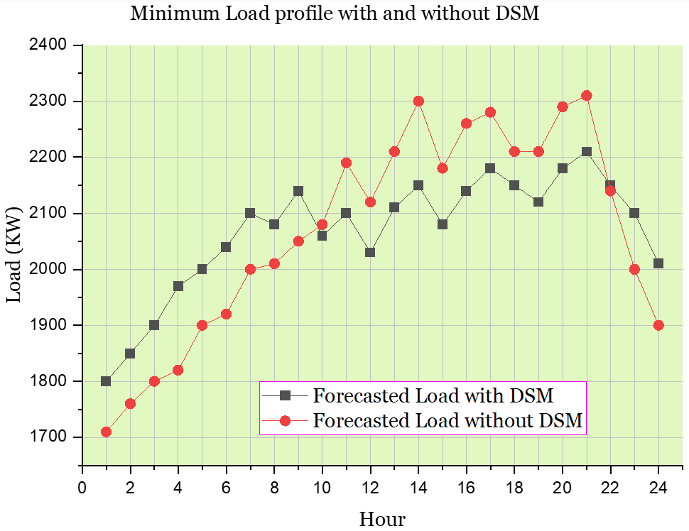
3. Demand-Side Management Modelling

For microgrid consumers, the daily electricity rates are scheduled one day in advance. Consumers are anticipated to alter their load demand in accordance with the pricing, following the price-elastic demand attributes, specified in these electricity costs. The equation that accounts for the responding load demand $P_D$ to switching power prices $P_r^e$ is [50].

$$P_D=\varphi \times P_r^e$$

(7)

Here, $\varphi$ is constant and using historic load information, and an individual may determine the price elasticity of load demand $\left(e\right)$. After demand response implementation, the anticipated actual and reactive energy use of loads can be calculated as follows

$${\stackrel{⌢}{P}}_{i,t}^{D_P}=\left[{\displaystyle \sum _{t=1}^T{\displaystyle \sum _{j=1}^J{\gamma }_{j,t}{Ŗ}_j}}\right]{\stackrel{⌢}{P}}_{i,t}^D$$

(8)

$${\stackrel{⌢}{Q}}_{i,t}^{D_P}=\left[{\displaystyle \sum _{t=1}^T{\displaystyle \sum _{j=1}^J{\gamma }_{j,t}{Ŗ}_j}}\right]{\stackrel{⌢}{Q}}_{i,t}^D$$

(9)

Here, load demand with demand response is expressed by ${\stackrel{⌢}{P}}_{i,t}^{D_P},\&{\stackrel{⌢}{Q}}_{i,t}^{D_P}$; and without demand response, it is ${\stackrel{⌢}{P}}_{i,t}^D,\&{\stackrel{⌢}{Q}}_{i,t}^D$. Binary selection ${\gamma }_{j,t}$ and the rate of DR on the cost status ${Ŗ}_j$. $\left(\stackrel{⌢}{•}\right)$ are unpredictability factors. Power grid dynamics are positively impacted by the introduction of battery energy storage systems (BESS) in combination with distributed generation (DG). BESS helps maintain the equilibrium between the irregular power generated by renewable systems and the load demand that uses the power, supporting the stability of the grid network. By supporting grid network operations like voltage stability control, load shifting, load levelling, and peak shaving, BESS facilitates the demand-side management (DSM) process. Customers who use BESS benefit from the ability to store electricity and discharge it as needed. The quantity of extra electricity required from the grid eventually decreases. SoC and DoD are two scientific abbreviations commonly used to describe the BESS state. The DoD is computed with BESS power $P_{BESS,k,t}$ as follows

$$DoD=\left(\left|P_{BESS,k,t}\right|t\right)/\left(E_{cap,k}\right)$$

(10)

Here, $E_{cap,k}$ is capacity of BESS. In [51], it is stated that the following might be used to express the connection between the BESS cycle life and DoD.

$$L\left(DoD\right)=x\times {\left(DoD\right)}^{-y}\mathit{exp}\left(-z\times DoD\right);x,y,z>0$$

(11)

Here, $x,y,z$ are factors and $L\left(DoD\right)$ is BESS life cycle function. The cost of battery degradation for the DoD is calculated as

$$C{F}_{\mathrm{de}r}\left(DoD\right)=\frac{C{F}_{BESS,k}\left|P_{BESS,k,t}\right|t}{2L\left(DoD\right)E_{cap}DoD{\eta }_c{\eta }_d}$$

(12)

Here, $C{F}_{BESS,k}$ is BESS substitute price, ${\eta }_c,{\eta }_d$ is efficiency of charging and discharging, and $C{F}_{\mathrm{de}r}\left(DoD\right)$ is a function of DoD to compute the degradation price of BESS. The conceptual framework for the overall BESS operating limitations is as follows:

$${ß}_{c,k,t}{P}_{c,k,min,t}\le P_{c,k,t}\le {ß}_{c,k,t}{P}_{c,k,max,t};t\in T,k\in N_{BESS}$$

(13)

$${ß}_{d,k,t}{P}_{d,k,min,t}\le P_{d,k,t}\le {ß}_{d,k,t}{P}_{d,k,max,t};t\in T,k\in N_{BESS}$$

(14)

$${ß}_{c,k,t}+{ß}_{d,k,t}\le 1;t\in T,k\in N_{BESS}$$

(15)

$$P_{BESS,k,t}=P_{c,k,t}{\eta }_c-\left(\frac{P_{d,k,t}}{{\eta }_d}\right);t\in T$$

(16)

$$E_{BESS,k,t}=E_{BESS,k,t-1}+P_{BESS,k,t};t\in T,k\in N_{BESS}$$

(17)

$$So{C}_{BESS,down,t}\le \left(E_{BESS,t}/E_{cap,t}\right)\le So{C}_{BESS,up,t};t\in T,k\in N_{BESS}$$

(18)

$$E_{BESS,k,24}=E_{BESS,k,o};k\in N_{BESS}$$

(19)

Here, the charge–discharge of the k^th battery in time t judgment is indicated by ${ß}_{c,k,t}$, ${ß}_{d,k,t}$; $P_{c,k,min,t}$, $P_{d,k,max,t}$, $P_{d,k,min,t}$, and $P_{c,k,max,t}$, are the min–max discharge–charge limits; $So{C}_{BESS,down,t}$, $So{C}_{BESS,up,t}$ are the lower and upper limits of state of charge; $E_{BESS,k,o}$ is the starting stored charge in the k^th BESS unit; $E_{BESS,k,24}$ is the remnant power in the final time interval; and $E_{BESS,k,t}$ denotes the BESS energy.

4. Problem Formulation

In the optimum problem solving situation, several state variables involving slack bus power $P_{slack}$, load bus voltage $V_{\mathcal{L},\mathcal{P}\mathcal{Q}}$, reactive power delivered by the DE-SG unit $Q_{\mathcal{D}\mathcal{E}-\mathcal{S}\mathcal{G},{\mathcal{N}}_{\mathcal{D}\mathcal{E}-\mathcal{S}\mathcal{G}}}$, solar unit $Q_{SP\mathcal{V},{\mathcal{N}}_{SP\mathcal{V}}}$, BESS unit $Q_{BESS,{\mathcal{N}}_{BESS}}$, and line loading ${\mathcal{S}}_{\mathcal{L},\mathcal{T}\mathcal{L}}$ are identified as follows

$$S^T=\left[\begin{array}{l}{P}_{slack},V_{\mathcal{L},1},\dots ,V_{\mathcal{L},{\mathcal{N}}_{\mathcal{P}\mathcal{Q}}},Q_{DE-SG,1},\dots ,Q_{DE-SG,{\mathcal{N}}_{DE-SG}},Q_{SP\mathcal{V},1},\dots ,\\ Q_{SP\mathcal{V},{\mathcal{N}}_{SP\mathcal{V}}},Q_{BESS,1},\dots ,Q_{BESS,{\mathcal{N}}_{BESS}},{\mathcal{S}}_{\mathcal{L},1},\dots ,{\mathcal{S}}_{\mathcal{L},{\mathcal{N}}_{\mathcal{T}\mathcal{L}}}\end{array}\right]$$

(20)

In addition, control variables involving DE-SG generator real power output $P_{\mathcal{D}\mathcal{E}-\mathcal{S}\mathcal{G},{\mathcal{N}}_{\mathcal{D}\mathcal{E}-\mathcal{S}\mathcal{G}}}$ excluding the slack bus, power of the solar PV units $P_{SP\mathcal{V},{\mathcal{N}}_{SP\mathcal{V}}}$, power of the BESS units $P_{BESS,{\mathcal{N}}_{BESS}}$, generator bus voltage $V_{G,\mathcal{P}\mathcal{V}}$, and transformer tap setting $T_{\mathcal{N}\mathcal{T}}$ are identified as follows

$$C^T=\left[\begin{array}{l}{P}_{\mathcal{D}\mathcal{E}-\mathcal{S}\mathcal{G},2},\dots P_{\mathcal{D}\mathcal{E}-\mathcal{S}\mathcal{G},{\mathcal{N}}_{\mathcal{D}\mathcal{E}-\mathcal{S}\mathcal{G}}},P_{SP\mathcal{V},1},\dots ,P_{SP\mathcal{V},{\mathcal{N}}_{SP\mathcal{V}}},\\ P_{BESS,1},\dots ,P_{BESS,{\mathcal{N}}_{BESS}},V_{G,1},\dots ,V_{G,{\mathcal{N}}_{\mathcal{P}\mathcal{V}}},T_1,\dots ,T_{{\mathcal{N}}_{\mathcal{N}\mathcal{T}}}\end{array}\right]$$

(21)

Here, ${\mathcal{N}}_{\mathcal{P}\mathcal{Q}}$ indicates the number of load buses, ${\mathcal{N}}_{\mathcal{P}\mathcal{V}}$ indicates the generator buses, ${\mathcal{N}}_{\mathcal{T}\mathcal{L}}$ indicates the power lines, and ${\mathcal{N}}_{\mathcal{N}\mathcal{T}}$ indicates the tap changing transformers in the system. Also indicated are the total number of power-generating units of DE-SG units ${\mathcal{N}}_{\mathcal{D}\mathcal{E}-\mathcal{S}\mathcal{G}}$, solar units ${\mathcal{N}}_{SP\mathcal{V}}$, and BESS units ${\mathcal{N}}_{\mathcal{B}\mathcal{E}\mathcal{S}\mathcal{S}}$.

The first objective of the work is to find the optimum total operational cost of AC/DC MG. The work focuses on the grid-connected mode of operation of MGs, which is also connected to DE-DG, SPV, and BESS for fulfilling the power demand. The objective function examines the hourly demand management by scheduling the generated power from the AC/DC MG power sources and utility optimally and economically. An objective function to be minimized, i.e., the optimum total operational cost, which comprises the minimum hourly generation cost and operational and maintenance (O&M) cost of power sources, can be represented as follows

$${ƒ}_{Obj,1}=min\hspace{0.17em}\hspace{0.17em}\mathcal{C}F\left(P\right)={\displaystyle \sum _{t=1}^{\mathcal{T}}\left[\begin{array}{l}\mathcal{C}{F}_{{\mathcal{D}\mathcal{E}}_{⬝}\mathcal{S}\mathcal{G}}\left(P_{{\mathcal{D}\mathcal{E}}_{⬝}\mathcal{S}\mathcal{G},k}\right)+\mathcal{C}{F}_{\mathcal{S}\mathcal{P}\mathcal{V}}\left(P_{\mathcal{S}\mathcal{P}\mathcal{V},k}\right)+\\ \mathcal{C}{F}_{\mathcal{B}\mathcal{E}\mathcal{S}\mathcal{S}}\left(P_{\mathcal{B}\mathcal{E}\mathcal{S}\mathcal{S},k}\right)+\mathcal{C}{F}_{\mathcal{G}rid}\left(P_{\mathcal{G}rid}\right)-\mathcal{C}{F}_{rev}\left(P_{rev}\right)\end{array}\right]}$$

(22)

Here, CF denotes the price or income of various microgrid components; $P_{{\mathcal{D}\mathcal{E}}_{⬝}\mathcal{S}\mathcal{G},k}$, $P_{\mathcal{S}\mathcal{P}\mathcal{V},k}$, $P_{\mathcal{B}\mathcal{E}\mathcal{S}\mathcal{S},k}$, $P_{\mathcal{G}rid}$, and $P_{rev}$ are the output power of DE-SG, SPV, BESS, Grid, and reserve, respectively. The DE-SG cost function can be represented as follows

$$\mathcal{C}{F}_{DE-SG}\left(P_{{\mathcal{D}\mathcal{E}}_{⬝}\mathcal{S}\mathcal{G},k}\right)={\displaystyle \sum _{k=1}^{{\mathcal{N}}_{{\mathcal{D}\mathcal{E}}_{⬝}\mathcal{S}\mathcal{G}}}\left(a_k+b_k{P}_{{\mathcal{D}\mathcal{E}}_{⬝}\mathcal{S}\mathcal{G},k}+c_k{P}_{{\mathcal{D}\mathcal{E}}_{⬝}\mathcal{S}\mathcal{G},k}^2\right)}$$

(23)

The renewable uncertainties cost model can be described by two cost models, the underestimation model and the overestimation model. A surplus of solar generation because of underestimation may create a problem relating to utility, like transmission line crowding, which tends to solar generator power restriction during routine operation. As per electricity market structure, solar farm operators are compensated, which is known as the underestimated cost. The overestimation of solar costs occurs when the real wind-generated energy is undersized with respect to the planned solar energy. As a consequence, there is insufficient electricity to meet the load’s requirement. A spinning reserve can be used to meet that need, whereas the underestimation of solar costs occurs when the real solar-generated energy is oversized with respect to the scheduled or planned solar energy. The system must be balanced to accommodate this additional energy. The cost functions are formulated as

$$\mathcal{C}{F}_{\mathcal{S}\mathcal{P}\mathcal{V}}\left(P_{\mathcal{S}\mathcal{P}\mathcal{V},k}\right)=\mathcal{D}\mathcal{C}F\left(P_{SP\mathcal{V},k}\right)+UC{F}_{SP\mathcal{V},k}^{UE}+OC{F}_{SP\mathcal{V},k}^{OE}\left(P_{SP\mathcal{V},k}\right)$$

(24)

$$min\hspace{0.17em}\hspace{0.17em}\mathcal{D}\mathcal{C}F\left(P_{SP\mathcal{V},k}\right)={\displaystyle \sum _{k=1}^{{\mathcal{N}}_{SP\mathcal{V}}}\left[\mathcal{D}\mathcal{C}F\left(P_{SP\mathcal{V},k}\right)\right]}={\displaystyle \sum _{k=1}^{{\mathcal{N}}_{SP\mathcal{V}}}\left[{\zeta }_{SP\mathcal{V},k}\times P_{SP\mathcal{V},k}\right]}$$

(25)

$$UC{F}_{SP\mathcal{V},k}^{UE}\left(P_{SP\mathcal{V},k}\right)=C_{SP\mathcal{V},k}^{UE}\left(P_{SP\mathcal{V},k}^A-P_{SP\mathcal{V},k}^S\right)$$

(26)

$$UC{F}_{SP\mathcal{V},k}^{UE}\left(P_{SP\mathcal{V},k}\right)=C_{SP\mathcal{V},k}^{UE}{\displaystyle {\int }_{P_{SP\mathcal{V},k}^S}^{P_{SP\mathcal{V},k}^R}\left(P_{SP\mathcal{V},k}-P_{SP\mathcal{V},k}^S\right){ƒ}_{SP\mathcal{V}}\left(P_{SP\mathcal{V},k}\right)d{P}_{SP\mathcal{V},k}}$$

(27)

$$OC{F}_{SP\mathcal{V},k}^{OE}\left(P_{SP\mathcal{V},k}\right)=C_{SP\mathcal{V},k}^{OE}\left(P_{SP\mathcal{V},k}^S-P_{SP\mathcal{V},k}^A\right)$$

(28)

$$OC{F}_{SP\mathcal{V},k}^{OE}\left(P_{SP\mathcal{V},k}\right)=C_{SP\mathcal{V},k}^{OE}{\displaystyle {\int }_{P_{SP\mathcal{V},k}^S}^{P_{SP\mathcal{V},k}^R}\left(P_{SP\mathcal{V},k}^S-P_{SP\mathcal{V},k}\right){ƒ}_{SP\mathcal{V}}\left(P_{SP\mathcal{V},k}\right)d{P}_{SP\mathcal{V},k}}$$

(29)

Here, $\mathcal{D}\mathcal{C}F\left(P_{SP\mathcal{V},k}\right)$, $P_{SP\mathcal{V},k}$, and ${\zeta }_{SP\mathcal{V},k}$ are described as the direct cost function of solar PV, generated solar PV power, and uncertainties cost coefficient of the $k^{th}$ PV unit of solar farm, respectively. $UC{F}_{SP\mathcal{V},k}^{UE}\left(P_{SP\mathcal{V},k}\right)$ is the stated underestimation cost; $OC{F}_{SP\mathcal{V},k}^{OE}\left(P_{SP\mathcal{V},k}\right)$ is the stated overestimation cost of $k^{th}$ solar PV unit; $C_{SP\mathcal{V}}^{UE}$ and $C_{SP\mathcal{V}}^{OE}$ define the uncertainties cost factors; $P_{SP\mathcal{V},k}^S$, $P_{SP\mathcal{V},k}$, $P_{SP\mathcal{V},k}^R$ and $P_{SP\mathcal{V},k}^A$ define the scheduled, generated, rated, and exciting PV power of the $k^{th}$ solar PV unit, respectively. Lognormal distribution accurately describes the distribution of irradiance $\left(Z_{SP\mathcal{V}}\right)$. To model the solar irradiation uncertainty, the Log-Normal probability distribution function is used which is function of solar irradiation $Z_{SP\mathcal{V}}$ can be indicated by following equation

$${ƒ}_{SP\mathcal{V}}\left(Z_{SP\mathcal{V},k}\right)=\left(\frac{1}{Z_{SP\mathcal{V}}\sqrt{2\pi \ast ln\left(1+\frac{{\partial }^2}{{\sigma }^2}\right)}}\right)exp\left[-0.5{\left\{\frac{ln\left(Z_{SP\mathcal{V}}\right)-ln\left(\sigma \right)+0.5ln\left(1+\frac{{\partial }^2}{{\sigma }^2}\right)}{\sqrt{ln\left(1+\frac{{\partial }^2}{{\sigma }^2}\right)}}\right\}}^2\right]\hspace{0.17em};\hspace{0.17em}\{Z_{SP\mathcal{V}}>0\}$$

(30)

Here, $\partial$ and $\sigma$ represent the mean and standard deviation, respectively, which are specified in Table 4. The solar PV output power $P_{SP\mathcal{V},k}$ is described by the following equation for irradiation $Z_{SP\mathcal{V}}$

$$P_{SP\mathcal{V},k}=\left\{\begin{array}{l}{P}_{SP\mathcal{V},k}^R\times \frac{{\left(Z_{SP\mathcal{V}}\right)}^2}{Z_{SP\mathcal{V}}^{St}\times Z_{SP\mathcal{V}}^C}\hspace{0.17em}\hspace{0.17em}\hspace{0.17em};\hspace{0.17em}\left(0<Z_{SP\mathcal{V}}<Z_{SP\mathcal{V}}^C\right)\\ P_{SP\mathcal{V},k}^R\left(\frac{Z_{SP\mathcal{V}}}{Z_{SP\mathcal{V}}^{St}}\right)\hspace{0.17em}\hspace{0.17em}\hspace{0.17em}\hspace{0.17em}\hspace{0.17em};\hspace{0.17em}\left(Z_{SP\mathcal{V}}\ge Z_{SP\mathcal{V}}^C\right)\end{array}\right.\hspace{0.17em}\hspace{0.17em}$$

(31)

Here, $Z_{SP\mathcal{V}}^{St}$ and $P_{SP\mathcal{V},k}^R$ define the standard solar irradiation and rated power of the $k^{th}$ solar PV unit, which are specified in Table 2. $Z_{SP\mathcal{V}}^C$ is a certain irradiance select as $180\hspace{0.17em}\hspace{0.17em}\mathrm{w}/{\mathrm{m}}^2$. For the estimation of solar power probabilities, the following equation are used

$${\rm P}r\left(P_{SP\mathcal{V},k}\right)=\frac{0.5}{\sqrt{\frac{P_{SP\mathcal{V},k}^R\times P_{SP\mathcal{V},k}}{Z_{SP\mathcal{V}}^{St}\times Z_{SP\mathcal{V}}^C}}}\left[{\rm P}{r}_Z\left(\sqrt{\frac{P_{SP\mathcal{V},k}\times Z_{SP\mathcal{V}}^{St}\times Z_{SP\mathcal{V}}^C}{P_{SP\mathcal{V},k}^R}}\right)+{\rm P}{r}_Z\left(-\sqrt{\frac{P_{SP\mathcal{V},k}\times Z_{SP\mathcal{V}}^{St}\times Z_{SP\mathcal{V}}^C}{P_{SP\mathcal{V},k}^R}}\right)\right]$$

(32)

The BESS cost function can be represented as follows

$$\mathcal{C}F\left(P_{\mathcal{B}\mathcal{E}\mathcal{S}\mathcal{S}}\right)={\displaystyle \sum _{k=1}^{{\mathcal{N}}_{\mathcal{B}\mathcal{E}\mathcal{S}\mathcal{S},k}}\left[{\mathcal{B}}_{\mathcal{B}\mathcal{E}\mathcal{S}\mathcal{S},k}\times {\chi }_{\mathcal{B}\mathcal{E}\mathcal{S}\mathcal{S},k}\times P_{\mathcal{B}\mathcal{E}\mathcal{S}\mathcal{S},k}\right]}$$

(33)

Here, ${\chi }_{\mathcal{B}\mathcal{E}\mathcal{S}\mathcal{S},k}$ indicate the status of BESS; ${\mathcal{B}}_{\mathcal{B}\mathcal{E}\mathcal{S}\mathcal{S},k}$ is the bid for BESS.

$$\mathcal{T}\mathcal{C}F\left(P_{\mathcal{B}\mathcal{E}\mathcal{S}\mathcal{S}}\right)=\frac{\mathcal{C}{F}_{\mathcal{B}\mathcal{E}\mathcal{S}\mathcal{S},max}}{365}\left[\frac{\mathcal{R}{\left(1+\mathcal{R}\right)}^{LT}}{{\left(1+\mathcal{R}\right)}^{LT}-1}\mathcal{C}{F}_{\mathcal{B}\mathcal{E}\mathcal{S}\mathcal{S}}+M\mathcal{C}{F}_{\mathcal{B}\mathcal{E}\mathcal{S}\mathcal{S}}\right]$$

(34)

The total cost per day of BESS is again an essential component of an optimum cost function. Here, BESS cost has been formulated by the fact that the cost of BESS depends on two essential elements. The first is the fixed cost of BESS, which includes the price of small battery blocks for setting up BESS and is only taken into consideration once. Annual maintenance cost (MC) is the second element that varies directly with BESS’s size. The cost function complies with the concepts mentioned above to calculate the total cost of BESS (in USD/day). $\mathcal{C}{F}_{\mathcal{B}\mathcal{E}\mathcal{S}\mathcal{S},max}$ is the size of BESS, which is subsequently optimized during the process, and LT is the lifetime, while $\mathcal{R}$ is the rate of interest for financing the installed BESS.

The cost function of the utility grid can be represented as follows

$$\mathcal{C}{F}_{\mathcal{G}rid}\left(P_{\mathcal{G}rid}\right)={\displaystyle \sum _{t=1}^T\left[\mathcal{C}{F}_{\mathcal{G}rid}^{buy}\left(t\right)P_{\mathcal{G}rid}^{lac}\left(t\right)-\mathcal{C}{F}_{\mathcal{G}rid}^{sell}\left(t\right)P_{\mathcal{G}rid}^{exs}\left(t\right)\right]}$$

(35)

The cost function of the reserve power can be represented as follows

$$\mathcal{C}{F}_{rev}\left(P_{rev}\right)={\displaystyle \sum _{t=1}^T{\displaystyle \sum _{i=1}^I{\displaystyle \sum _{j=1}^J\left[\mathcal{C}{F}_{r,j}\left(t\right)P_{i,t}^D{\gamma }_{j,t}{Ŗ}_{j}t\right]}}}\hspace{0.17em};\hspace{0.17em}{\gamma }_{j,t}\in \left\{0,1\right\}\forall j,t$$

(36)

$$\mathcal{C}{F}_{rev}\left(P_{rev}\right)\le {\displaystyle \sum _{t=1}^{\mathcal{T}}{\displaystyle \sum _{i=1}^{\mathcal{I}}\left[\mathcal{C}{F}_{r,0}\left(t\right)P_{i,t}^{D}t\right]}}$$

(37)

$${\displaystyle \sum _{t=1}^T{\displaystyle \sum _{i=1}^I{\displaystyle \sum _{j=1}^J\left[P_{i,t}^{LD}{\gamma }_{j,t}{Ŗ}_{j}t\right]}}}\ge {\displaystyle \sum _{t=1}^T{\displaystyle \sum _{i=1}^I\left[P_{i,t}^{D}t\right]}}$$

(38)

$$P_{i+1,t}=P_{i,t}-P_{i,t}^{lat}-{\stackrel{⌢}{P}}_{i,t}^{D_P}-P_{i,t}^{ch}-P_{i,t}^{dis}+{\stackrel{⌢}{P}}_{i,t}^{SPV};\forall i,t$$

(39)

$$Q_{i+1,t}=Q_{i,t}-Q_{i,t}^{lat}-{\stackrel{⌢}{Q}}^{D_P};\forall i,t$$

(40)

$$V_{i+1,t}=V_{i,t}-\frac{R_{i,}{P}_{i,,t}+X_i{Q}_{i,,t}}{V_0};\forall i,,t$$

(41)

$$P_{1,t}=P_t^{def}-P_t^{sur};P_t^{def}\ge 0;P_t^{sur}\ge 0;\forall t$$

(42)

$$P_{i,t}^2+Q_{i,t}^2\le S_i^2;\forall i,t$$

(43)

Here, $\mathcal{C}{F}_{\mathcal{G}rid}^{buy}$ and $\mathcal{C}{F}_{\mathcal{G}rid}^{sell}$ denote the cost of buying/selling power from/to the utility grid. $\mathcal{C}{F}_{r,0}$ is authentic cost for consumers without DSM. $P_{\mathcal{G}rid}^{lac}$ and $P_{\mathcal{G}rid}^{exs}$ are the lack of and excess power of AC/DC MG. $P_{i,t}^{lat}$ and $Q_{i,t}^{lat}$ are the real/reactive power transfer from bus i through the lateral branch $i$. $P_{i,t}^{ch}$ and $P_{i,t}^{dis}$ are the BESS power before DSM. $\stackrel{⌢}{P}$ denote the power after DSM. $R_{i,}$ and $X_i$ are the line impedance (ohm). $V_{i,t}$ is the bus voltage. The goal is to reduce the overall AC/DC MG running costs. The entire O&M costs of DE-SG, SPV, and BESS are calculated, accordingly, in Equation (30) through (31)–(42). The transaction cost using the primary grid is calculated in Equation (43). Additionally, Equation (44), with the demand response in place, computes the revenues from selling electricity to the subscribers. Constraint (45) states that the binary nature of the demand response decision variables, and Constraint (46) establishes a limit on the number of active demand response levels per hour. Security limits (47) and (48) state that customers’ electricity usage cannot be negatively influenced by the demand response and that electricity bills for consumers after the implementation of the demand response cannot be higher than the initial bills. A linearized distribution load flow model is shown in Equations (47)–(51).

Mathematically, an improved objective function can be stated as follows

$$min\hspace{0.17em}\hspace{0.17em}{ƒ}_{Obj,2}=\left\{\begin{array}{l}{f}_{Obj}+{\lambda }_{P_{slack}}{\left(P_{slack}-P_{slack}^{lim}\right)}^2+{\lambda }_{{\mathcal{Q}}_{{\mathcal{N}}_{\mathcal{D}\mathcal{E}-\mathcal{S}\mathcal{G}}}}{\displaystyle \sum _{k=1}^{{\mathcal{N}}_{\mathcal{D}\mathcal{E}-\mathcal{S}\mathcal{G}}}{\left(Q_{\mathcal{D}\mathcal{E}-\mathcal{S}\mathcal{G},k}-Q_{\mathcal{D}\mathcal{E}-\mathcal{S}\mathcal{G},k}^{lim}\right)}^2}+{\lambda }_{\mathcal{V}\mathcal{P}\mathcal{Q}}{\displaystyle \sum _{k=1}^{{\mathcal{N}}_{\mathcal{P}\mathcal{Q}}}{\left(V_{\mathcal{L},k}-V_{\mathcal{L},k}^{lim}\right)}^2+}\\ {\lambda }_{{\mathcal{Q}}_{{\mathcal{N}}_{SP\mathcal{V}}}}{\displaystyle \sum _{k=1}^{{\mathcal{N}}_{SP\mathcal{V}}}{\left(Q_{SP\mathcal{V},k}-Q_{SP\mathcal{V},k}^{lim}\right)}^2}+{\lambda }_{{\mathcal{Q}}_{{\mathcal{N}}_{BESS}}}{\displaystyle \sum _{k=1}^{{\mathcal{N}}_{BESS}}{\left(Q_{BESS,k}-Q_{BESS,k}^{lim}\right)}^2}+{\lambda }_{\mathcal{Q}{\mathcal{S}}_{\mathcal{L}}}{\displaystyle \sum _{k=1}^{{\mathcal{N}}_{\mathcal{N}\mathcal{T}}}{\left({\mathcal{S}}_{\mathcal{L},k}-{\mathcal{S}}_{\mathcal{L},k}^{lim}\right)}^2}\end{array}\right\}$$

(44)

$$x^{lim}=\left\{\begin{array}{l}{x}^{max}x>x^{max}\\ x^{min}x<x^{min}\end{array}\right.$$

(45)

Here, ${\lambda }_{P_{slack}}, {\lambda }_{{\mathcal{Q}}_{{\mathcal{N}}_{\mathcal{D}\mathcal{E}-\mathcal{S}\mathcal{G}}}}, {\lambda }_{\mathcal{V}\mathcal{P}\mathcal{Q}}, {\lambda }_{{\mathcal{Q}}_{{\mathcal{N}}_{SP\mathcal{V}}}}, {\lambda }_{{\mathcal{Q}}_{{\mathcal{N}}_{BESS}}},\hspace{0.17em}\&\hspace{0.17em}{\lambda }_{\mathcal{Q}{\mathcal{S}}_{\mathcal{L}}}$ are penalty components, set as 1000. $x^{lim}$ is the limiting value of control parameter, x. If x is greater than the upper limit, $x^{lim}$ keeps to the upper limit, and if x is less than the lower limit, $x^{lim}$ keeps to the lower limit point.

4.1. Total Emission Minimization Model

For the minimization of emissions, the objective function of the cost model inclusive of tax is represented as follows

$$min\hspace{0.17em}\hspace{0.17em}{ƒ}_{Obj,2}={ƒ}_{Obj,1}+\left[{\mathcal{C}}_{\lambda }\ast EF\left(P_{\mathcal{D}\mathcal{E}-\mathcal{S}\mathcal{G},k}\right)\right]$$

(46)

4.2. Total Active Power Losses Minimization

Toward the objective of a reduction in the active power losses of the power system, an objective function can be expressed as follows

$$min\hspace{0.17em}\hspace{0.17em}{ƒ}_{Obj,3}=P_L=\left[{\displaystyle \sum _{k=1}^{{\mathcal{N}}_{\mathcal{D}\mathcal{E}-\mathcal{S}\mathcal{G}}}\left(P_{\mathcal{D}\mathcal{E}-\mathcal{S}\mathcal{G},k}\right)}+{\displaystyle \sum _{k=1}^{{\mathcal{N}}_{BESS}}\left(P_{BESS,k}\right)}+{\displaystyle \sum _{k=1}^{{\mathcal{N}}_{SP\mathcal{V}}}\left(P_{SP\mathcal{V},k}\right)}\right]-{\displaystyle \sum _{k=1}^{{\mathcal{N}}_{\mathcal{P}\mathcal{Q}}}\left(P_{D,k}\right)}$$

(47)

In the above relation, the total load demand is defined by $P_D$ and the loss of the transmission loss by $P_L$. The total number of buses in the system is denoted by ${\mathcal{N}}_{bus}$. $G_m$ denotes the conductance of the line $m$ connecting buses $r\hspace{0.17em}\&\hspace{0.17em}t$; $V_r^{}\hspace{0.17em}\&\hspace{0.17em}{V}_t^{}$ are the voltage at bus buses $r\hspace{0.17em}\&\hspace{0.17em}t$ respectively; ${\Phi }_{rt}$ is the angle between buses.

4.3. Voltage Deviation Minimization

The next objective is to consider the reduction in deviation in the voltage at $\mathcal{P}\mathcal{Q}$ buses from the reference voltage of $1\hspace{0.17em}p.u.$ and can be represented as follows [52]

$$min\hspace{0.17em}\hspace{0.17em}{ƒ}_{Obj,4}=VD={\displaystyle \sum _{m=1}^{{\mathcal{N}}_{\mathcal{P}\mathcal{Q}}}\left[V_m-V_m^{ref}\right]}$$

(48)

Here, $V_m^{ref}$ is the reference voltage at the $m^{th}$ load bus and is set at $1\hspace{0.17em}p.u.$ generally.

4.4. Security Constraints

In this study, we considered several realistic security constraints for solving the scheduling and optimal power flow problem. Equality limits usually consist of active and reactive power balance equations at every node. These constraints equations are given below.

$${\displaystyle \sum P_k}=0\hspace{0.17em};\hspace{0.17em}and\hspace{0.17em}{\displaystyle \sum Q_k}=0$$

(49)

Here $P_k$ and $Q_k$ represent, respectively, the net real and imaginary power injections at the $k^{th}$ node.

(a)

Generators limits

The operating limits of the thermal generators may be stated as below

$$P_{\mathcal{D}\mathcal{E}-\mathcal{S}\mathcal{G},k}^{min}\le P_{\mathcal{D}\mathcal{E}-\mathcal{S}\mathcal{G},k}\le P_{\mathcal{D}\mathcal{E}-\mathcal{S}\mathcal{G},k}^{max}\hspace{0.17em}\hspace{0.17em}\hspace{0.17em}\forall k\in {\mathcal{N}}_{\mathcal{D}\mathcal{E}-\mathcal{S}\mathcal{G}}$$

(50)

$$Q_{\mathcal{D}\mathcal{E}-\mathcal{S}\mathcal{G},k}^{min}\le Q_{\mathcal{D}\mathcal{E}-\mathcal{S}\mathcal{G},k}\le Q_{\mathcal{D}\mathcal{E}-\mathcal{S}\mathcal{G},k}^{max}\hspace{0.17em}\hspace{0.17em}\hspace{0.17em}\forall k\in {\mathcal{N}}_{\mathcal{D}\mathcal{E}-\mathcal{S}\mathcal{G}}$$

(51)

$$P_{SP\mathcal{V},k}^{min}\le P_{SP\mathcal{V},k}\le P_{SP\mathcal{V},k}^{max}\hspace{0.17em}\hspace{0.17em}\hspace{0.17em}\forall k\in {\mathcal{N}}_{SP\mathcal{V}}$$

(52)

$$Q_{SP\mathcal{V},k}^{min}\le Q_{SP\mathcal{V},k}\le Q_{SP\mathcal{V},k}^{max}\hspace{0.17em}\hspace{0.17em}\hspace{0.17em}\forall k\in {\mathcal{N}}_{SP\mathcal{V}}$$

(53)

$$P_{Grid}^{min}\le P_{Grid}\le P_{Grid}^{max}\hspace{0.17em}\hspace{0.17em}\hspace{0.17em}$$

(54)

$$V_{G,k}^{min}\le V_{G,k}\le V_{G,k}^{max}\hspace{0.17em}\hspace{0.17em}\hspace{0.17em}\forall k\in {\mathcal{N}}_{\mathcal{P}\mathcal{V}}$$

(55)

(b)

Security limits

While minimizing objective function, it is necessary that the min and max limits of the voltage magnitude at load buses should remain within certain limits. Furthermore, the complex power in all transmission lines should not exceed their maximum limit. The boundary conditions associated with these variables are mathematically formulated in the following equations

$$V_{\mathcal{L},k}^{min}\le V_{\mathcal{L},k}\le V_{\mathcal{L},k}^{max}\hspace{0.17em}\hspace{0.17em}\hspace{0.17em}\forall k\in {\mathcal{N}}_{\mathcal{P}\mathcal{Q}}$$

(56)

$${\mathcal{S}}_{\mathcal{L},k}\le {\mathcal{S}}_{\mathcal{L},k}^{max}\hspace{0.17em}\hspace{0.17em}\forall k\in {\mathcal{N}}_{\mathcal{T}\mathcal{L}}$$

(57)

where ${\mathcal{S}}_{\mathcal{L},k}$ and ${\mathcal{S}}_{\mathcal{L},k}^{max}$ represent the apparent power flow limit of the transmission line, while superscripts, namely min and max, are associated with the different variables’ corresponding variable. Similarly, $V_{\mathcal{L},k}^{min}$ and $V_{\mathcal{L},k}^{max}$ represent the voltage values at load buses. An objective function equation is a quadratic penalty term. In the function given below, penalty terms represent the extent of the limit violation. The degree of the limit violation is positive when limits are violated and zero when they are not violated [53].

(c)

Constraints of DSM

To incorporate DSM into the problem, fresh demand has been created by shifting demand from one hour to another according to the need of the hour. The latest demand after the demand response, where the relocated demand is either connected $\left(dVa{r}_{i,t}^{up}\right)$ or deducted $\left(dVa{r}_{i,t}^{dn}\right)$ from the base load demand, can be expressed as follows

$$d{P}_{i,t}=P_{D_{i,t}}+dVa{r}_{i,t}^{up}-dVa{r}_{i,t}^{dn}$$

(58)

The load demand response is executed such that the share of the demand detached during the peak hours of the day should be identical to the share of the demand joined during off-peak hours and can be expressed as follows

$${\displaystyle \sum _{t=1}^{T}dVa{r}_{i,t}^{up}}={\displaystyle \sum _{t=1}^{T}dVa{r}_{i,t}^{dn}}$$

(59)

The part of the load demand to be attached or detached relies on the ratio of the demand response and can be expressed as follows

$$0\le dVa{r}_{i,t}^{up}\le B^{up}\times P_{D_{i,t}}$$

(60)

$$0\le dVa{r}_{i,t}^{dn}\le B^{dn}\times P_{D_{i,t}}$$

(61)

The load demand to be locomoted at someone’s chosen hour can be as undersized as zero and as great as the ratio demand response of the load to be satisfied.

(d)

Constraints of BESS

This section briefly discusses the limitations of storage devices for the proper functioning during the specified time span. The following equations and constraints have been formulated for the BESS system. The calculation of the amount of energy stored during the discharging and charging mode of the BESS can be expressed as follows

$$C_{BESS,t+1}=max\left\{\left(\frac{C_{BESS,t}-\Delta t{P}_{BESS,t}}{{\eta }_d}\right),C_{BESS,min}\right\};t=1,2,3,\dots ,T$$

(62)

$$C_{BESS,t+1}=min\left\{\left(C_{BESS,t}-\Delta t{P}_{BESS,t}{\eta }_c\right),C_{BESS,max}\right\};t=1,2,3,\dots ,T$$

(63)

The state of BESS (either charging or discharging) depends on the charge left in the previous hour after contributing power according to the demand. The power discharged or charged should be within the maximum and the minimum discharging/charging rates (in kW) and can be represented as follows

$$\underset{¯}{{\mathcal{R}}_{\mathcal{B}\mathcal{E}\mathcal{S}\mathcal{S},t}}\le P_{\mathcal{B}\mathcal{E}\mathcal{S}\mathcal{S},t}\le \overline{{\mathcal{R}}_{\mathcal{B}\mathcal{E}\mathcal{S}\mathcal{S},t}}$$

(64)

$$\underset{¯}{{\mathcal{R}}_{\mathcal{B}\mathcal{E}\mathcal{S}\mathcal{S},t}}=max\left\{\left(P_{\mathcal{B}\mathcal{E}\mathcal{S}\mathcal{S},min},\frac{\left(C_{\mathcal{B}\mathcal{E}\mathcal{S}\mathcal{S},t}-C_{\mathcal{B}\mathcal{E}\mathcal{S}\mathcal{S},max}\right)}{{\eta }_c\Delta t}\right)\right\}$$

(65)

$$\overline{{\mathcal{R}}_{\mathcal{B}\mathcal{E}\mathcal{S}\mathcal{S},t}}=min\left\{\left(P_{\mathcal{B}\mathcal{E}\mathcal{S}\mathcal{S},max},\frac{\left(C_{\mathcal{B}\mathcal{E}\mathcal{S}\mathcal{S},t}-C_{\mathcal{B}\mathcal{E}\mathcal{S}\mathcal{S},min}\right){\eta }_d}{\Delta t}\right)\right\}$$

(66)

(e)

Constraints of Operating Reserve

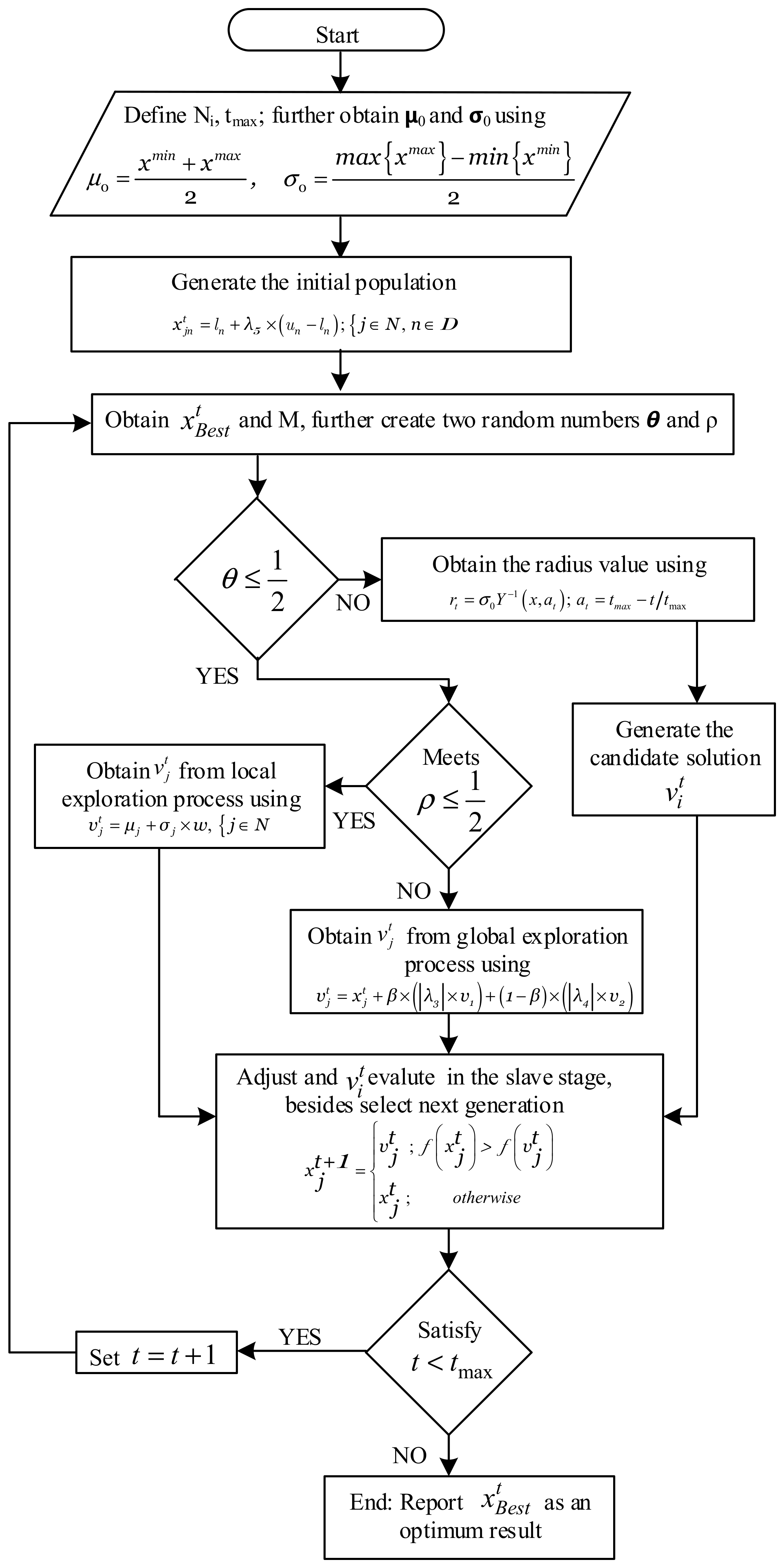
Operating reserve (OR) from SPV and BESS plays a significant role in the reliability enhancement of the AC/DC MG. It is defined as the hourly sum of the reserved capacity of power generation from BESS, SPV, and utility (when their status is ON). The maximum response time of OR to be fed to the MG is 10 min has been formulated as follows

$$P_{SPV,k,max}{u}_{SP\mathcal{V},k}+\overline{{\mathcal{R}}_{\mathcal{B}\mathcal{E}\mathcal{S}\mathcal{S},t}}{u}_{\mathcal{B}\mathcal{E}\mathcal{S}\mathcal{S},t}+P_{Grid,max}\ge O{R}_t+P_{D,t};t\in T$$

(67)

The load demand is obtained via the combination of all generators of AC/DC microgrids; however, from an economic perspective, the contribution is decided by values of the penalty cost. To validate the results of the minimum cost with the application of the generalized normal distribution optimization (GNDO) algorithm in terms of the best factor of the objective function obtained, result time, and total iterations, it is compared with the results of similar research work.

5. GNDO Algorithm

Normal distribution is a probability function that can be completely described with its mean and variance. Its wide adoption has to do with its simplicity in the formulation, and basically, every sample distribution that we would encounter in most situations would eventually follow a normal distribution if the sample size were large enough, and that is a nice property when we are modeling the stochastic behavior [38]. The normal distribution is a continuous probability distribution choosing a PDF specified by two parameters, $\mu$ and $\sigma$. The Greek symbol $\mu$ is the mean (arithmetic average) of the normal distribution. The Greek symbol $\sigma$ is the standard deviation which measures the spread of the distribution. The standard deviation is measured if the individual differences in the observations. Every normal distribution is characterized by the following facts: Approximately 66% of the data values in a normal distribution fall between $\left(\mu -1\sigma \right)$ and $\left(\mu +1\sigma \right)$. Approximately 95% of the data values in a normal distribution fall between $\left(\mu -2\sigma \right)$ and $\left(\mu +2\sigma \right)$. Approximately 99.7% of the data values in a normal distribution fall between $\left(\mu -3\sigma \right)$ and $\left(\mu +3\sigma \right)$. A lot of phenomena follow a similar distribution. That distribution turns out to be normal. So, we can look at it as the familiar bell-shaped curve (although not all bell-shaped curves are normal) but, for math and statistics, we need a formula. It turns out that the formula for the normal is rather messy [39]. For a random variable $x$, the probability density function (PDF) of normal distribution is expressed as

$$ƒ\left(x,\mu ,\sigma \right)=\frac{1}{\sqrt{2\pi }\sigma }exp\left(-\frac{{\left(x-\mu \right)}^2}{2{\sigma }^2}\right)$$

(68)

Figure 2 demonstrated the characteristics of the normal distribution of random variables against several values of $\mu$ and $\sigma$. An effective and simple optimization approach based on normal distribution, termed generalized normal distribution optimization (GNDO), is first proposed by Zhang 2020 [40], with special characteristics. Figure 3 demonstrates the methodology and search strategies of the GNDO.

GNDO has a very straightforward framework whose design consists of mainly two statistics-transferring approaches: the first is local exploitation, and the second is global exploration. In exploitation, a wide search is carried out to observe the greatest results established thus far to assay whether there are superior solutions in an effort to speed up convergence. Furthermore, in the generalized normal distribution model, local exploitation is assisted through the present average position and the present optimum position, whereas global exploration is associated with three randomly chosen agents.

In the local exploitation stage, an optimization model of the generalized normal distribution is a correlation between a normal distribution and the allocation of populations (individualistic) that can be formulated as

$$v_j^t={\mu }_j+{\sigma }_j\times w, \hspace{0.33em}\hspace{0.17em}\left\{j\in N\right\}$$

(69)

Here, $v_j^t$ is the trail vector of the $j^{th}$ individualistic at time $t$. ${\mu }_j$ and ${\sigma }_j$ define the generalized average location and the standard variance. $w$ is the penalty factor.

$${\mu }_j=\frac{1}{3}\left(x_j^t+x_{Best}^t+M\right)$$

(70)

$${\sigma }_j=\sqrt{\frac{1}{3}\left[{\left(x_j^t-\mu \right)}^2+{\left(x_{Best}^t-\mu \right)}^2+{\left(M-\mu \right)}^2\right]}$$

(71)

$$w=\left\{\begin{array}{l}\left(\sqrt{-\log \left({\lambda }_1\right)}\right)\cos \left(2\pi {\lambda }_2\right)\hspace{0.17em}\hspace{0.17em}\hspace{0.17em}\hspace{0.17em}\hspace{0.17em}\hspace{0.17em}\hspace{0.17em}\hspace{0.17em}\hspace{0.17em};\hspace{0.33em}if\hspace{0.33em}a\le b\\ \left(\sqrt{-\log \left({\lambda }_1\right)}\right)\cos \left(2\pi {\lambda }_2+\pi \right);\hspace{0.33em}otherwise\end{array}\right.$$

(72)

Here, $x_{Best}^t$ is the current optimum position; $a,\hspace{0.17em}b,\hspace{0.17em}{\lambda }_1,\hspace{0.17em}\&\hspace{0.17em}{\lambda }_2$ are random quantities $\left[0,\hspace{0.17em}1\right]$; and $M$ is the mean or average position of the present population that can be evaluated as

$$M=\frac{{\displaystyle \sum _{j=1}^N\left[x_j^t\right]}}{N}$$

(73)

The global exploration related to choosing three random populations can be described as

$$v_j^t=x_j^t+\underset{\mathrm{Locally} \mathrm{information}-\mathrm{sharing}}{\underbrace{\beta \times \left(\left|{\lambda }_3\right|\times v_1\right)}}+\hspace{0.17em}\underset{\mathrm{Globally} \mathrm{information}-\mathrm{sharing}}{\underbrace{\left(1-\beta \right)\times \left(\left|{\lambda }_4\right|\times v_2\right)}}$$

(74)

Here, ${\lambda }_3\hspace{0.17em}\&\hspace{0.17em}{\lambda }_4$ specify two random parameters associated with normal distribution; $\beta$ is the modifying constant, which is a random number $\left[0,\hspace{0.17em}1\right]$; $v_1\hspace{0.17em}\&\hspace{0.17em}{v}_2$ are the specified train vectors that can be assessed using following equation

$$v_1=\left\{\begin{array}{l}{x}_j^t-x_{k1}^t\hspace{0.33em};\hspace{0.33em}ƒ\left(x_j^t\right)<ƒ\left(x_{k1}^t\right)\\ x_{k1}^t-x_j^t\hspace{0.17em}\hspace{0.17em};\hspace{0.33em}otherwise\end{array}\right.$$

(75)

$$v_2=\left\{\begin{array}{l}{x}_{k2}^t-x_{k3}^t\hspace{0.33em}\hspace{0.33em};ƒ\left(x_{k2}^t\right)<ƒ\left(x_{k3}^t\right)\\ x_{k3}^t-x_{k2}^t\hspace{0.33em}\hspace{0.33em};\hspace{0.33em}\hspace{0.33em}otherwise\end{array}\right.$$

(76)

Here, $k_1,\hspace{0.17em}{k}_2,\hspace{0.17em}\&\hspace{0.17em}{k}_3$ are three random numbers $\left[1,\hspace{0.17em}N\right]$ that match $k_1\ne k_2\ne k_3\ne j$. In order to guarantee the viability of all generations in the solution area, the following equation is utilized

$$v_{j,r}^t=\left\{\begin{array}{l}{v}_{j,r}^t\hspace{0.17em}\hspace{0.17em}\hspace{0.17em};\hspace{0.33em}min\left(x_r^t\right)\le v_{j,r}^t\le max\left(x_r^t\right)\\ x_{best,r}^t\hspace{0.33em};\hspace{0.33em}\hspace{0.33em}\hspace{0.33em}\hspace{0.33em}\hspace{0.33em}\hspace{0.33em}\hspace{0.33em}\hspace{0.33em}otherwise\end{array}\right.$$

(77)

Here, $min\left(x_r^t\right),\hspace{0.17em}\&\hspace{0.17em}max\left(x_r^t\right)$ are the lowest and highest integer values associated with the set of decision variables, which are assessed from the initial position to next position of the vector $v_{j,r}^t$ using the decision variable $r$. $x_{best,r}^t$ refers to the value of the decision variable $r$ for the best present solution observed so far.

The execution of GNDO is related to the configured local exploitation and global exploration approaches. These approaches have the aforementioned significance to GNDO, which has an identical probability to be chosen. Therefore, similarly to other developed optimization techniques such as GWO, TLBO, PSO, WOA, CO, etc., the GNDO population is initialized using following equation

$$x_{jn}^t=l_n+{\lambda }_5\times \left(u_n-l_n\right)\hspace{0.17em};\hspace{0.17em}\hspace{0.17em}\left\{j\in N,\hspace{0.17em}\hspace{0.17em}n\in D\right\}\hspace{0.33em}$$

(78)

Here, $D$ defines the total numbers design variables; $l_n,\hspace{0.17em}\&\hspace{0.17em}{u}_n$ are the lower and upper boundary of the $n^{th}$ design variable; and ${\lambda }_5$ is a random number $\left[0,\hspace{0.17em}1\right]$. If a better solution cannot be found in a local exploitation strategy or a global exploration approach, then it is necessary to make better solutions for the succeeding generation, and thus, a screening technique is developed, which can be expressed as

$$x_j^{t+1}=\left\{\begin{array}{l}{v}_j^t\hspace{0.17em}\hspace{0.17em};\hspace{0.33em}ƒ\left(x_j^t\right)>ƒ\left(v_j^t\right)\\ x_j^t\hspace{0.33em};\hspace{0.33em}\hspace{0.33em}\hspace{0.33em}\hspace{0.33em}\hspace{0.33em}\hspace{0.33em}\hspace{0.33em}\hspace{0.33em}otherwise\end{array}\right.$$

(79)

Here, $x_j^{t+1}$ is the best solution, and $t,\hspace{0.17em}\hspace{0.17em}t+1$ indicate the current and next iteration value, respectively. The execution of GNDO is explained in a flowchart [54], as demonstrated in Figure 4.

6. Simulation Results Case Studies

In this section, to solve the proposed problems of Section 3, the GNDO algorithm is tested on grid-connected AC/DC microgrid study systems which including solar PV and BESS units. Figure 1 shows the study system. The simulations are run on a personal computer with three processors running at 3.0 GHz, with 1 TB of storage and 8 GB of RAM, and the algorithm is written in MATLAB. The population size is set at 50, the highest iteration number is set at 500, and 30 runs have been fixed for the algorithm, accordingly. Different cases are considered for the simulation study to verify the performance of the suggested GNDO algorithm. Furthermore, to ensure a fair comparative analysis among the achieved simulation solutions from the optimization methods, parameter settings of competing algorithms are taken uniformly such as the maximum number of iterations $T_{max}$, population size $N$, etc. The case simulations are prescribed as follows

Case 1:

Minimization optimum total operational cost without DSM.

Case 2:

Minimization emissions without DSM.

Case 3:

Minimization active power loss without DSM.

Case 4:

Minimization of voltage deviation (VD) without DSM.

Case 5:

Minimization optimum total operational cost with DSM.

Case 6:

Minimization emissions with DSM.

Case 7:

Minimization active power loss with DSM.

Case 8:

Minimization of voltage deviation (VD) with DSM.

6.1. Implementation of GNDO Algorithm for DSM of Grid-Connected AC/DC MGs

The GNDO algorithm has been used to find the optimum total operational cost, emissions, active power loss, and voltage deviation (VD) of a MG by optimally scheduling the power generated by DGs and utility on an hourly basis. The following steps discuss the process of implementing GNDO algorithm for the present work.

Step 1

All the essential input data (viz., power demand, upper and lower limits of power from DE-SG, SPV, BESS and utility, hourly output power of DE-SG, SPV and BESS, forecasted market price for an entire day, hourly bid for utility, and bids for SPV, BESS, and DE-SG) have been defined. Set the initial parameters of solution algorithm.

Step 2

The initial population (i.e., power generated by each element), adhering with (50)–(55) and (62)–(68) has been initialized.

Step 3

Generated power has been scheduled such that all security constraints are satisfied.

Step 4

The cost of the generated power of utility and each DE-SG, SPV, and BESS unit has been calculated using (22)–(37); emission is calculated using (46); total active power loss is calculated using (47); and voltage deviation is calculated using (48).

Step 5

Establish $x_j^{t+1}$ and set the iteration $itr=1$.

Step 6

The best solutions from the population for each element have been selected. Obtained new results utilizing (77)–(79) and rectify the results.

Step 7

Check whether the updated values of the specific problem are within the operating limits or not. The independent variable is considered as the least value, if it less with respect to the minimum value, and make it equivalent to the highest value if it is more than the most significant value.

Step 8

The best solution is found after updating of each solution for maximum number of iterations.

Step 9

The total cost and emission values are calculated using the final power output values. Stop the algorithm if $itr=maxitr$. The final optimal solution will be reached.

The above steps have been repeated by updating the new demand after considering a DR of 15% using (58)–(61). In this study, two scenarios of load demand, low load and high load, are considered. The total power demand of AC/DC MG is 49,650 kWh and 88,960 kWh for a day with low-load and high-load scenarios. The load demand curve with and without DSM for a day is presented in Figure 4 and Figure 5 for low- and high-load scenarios, respectively. According to the load profiles presented in Figure 5 and Figure 6, the final load curve, i.e., after load shifting is similar to the necessary objective curve in each of the two scenarios. It is worth noting that the distance between the target curve and the load curve has been successfully minimized by the GNDO algorithm. The proposed GNDO algorithm appears to be the most successful and efficient in providing a global optimal solution for lowering utility bill costs.

Table 5. Boundary values, emission, and bids factor of AC/DC MG units and utility.

AC/DC MG Units	Power (KW)		Cost			$\mathbf{Emission} \left(\mathbf{l}\mathbf{b}/\mathbf{k}\mathbf{W}\hspace{0.17em}\mathbf{h}\right)$
	$\mathit{m}\mathit{i}\mathit{n}.$	$\mathit{m}\mathit{a}\mathit{x}.$	Bidding (USD/kW h)	O&M (USD/kW h)	Start-Up/ Shut-Down (USD)	CO2	SO2	NOX
SPV-1	0	10.5	2.584	0.2082	0	-	-	-
SPV-2	0	725	2.584	0.2082	0	-	-	-
DE-SG	500	3000	0.457	0.04476	0.96	1.96211	0.0397	0.89
BESS-1	−96	96	0.380	-	-	0.02204	0.0002	0.001
BESS-2	−30	30	0.380	-	-	0.03114	0.0012	0.002
Utility	−1000	2000	-	-	-	2.09	0.0011	0.0046

shows the power limits for installed DGs, bidding cost (in USD/kWh), operation and maintenance cost (in USD/kWh) and the start-up/shut-down costs (in USD) of each DG. The cost involved in turning on and off the respective DG is included in the start-up and shut-down costs, respectively.

A scheduling horizon of 24 h has been chosen with each interval of one hour. The amount of CO₂, SO₂, and NO_x emissions from different DGs and utilities is presented in Table 5. After the utility, DE-SG’s emission is on the higher side followed by BESS. RESs, viz. SPV, do not produce any kind of emissions. In this work, tax is selected as 10%. The analysis has been performed on an hourly basis and the impact of 15% DR has been evaluated for the grid-connected mode of AC/DC MG. Peak load is subsequently reduced as a result of load shifting. As a result, it benefits both the utilities and the end users. Generators with higher ratings are mostly expensive, and their requirement is high when demand is at its peak. As after DSM, peak load decreases, the utility then realizes significant savings in terms of generation scheduling. The capacity for reserve generation consequently rises. The optimal simulation results for power flow in terms of minimization of operating cost, emission, power loss, and voltage deviation in grid-connected AC/DC MG are reported in

Table 6. Simulation results optimum power flow obtained via GNDO with and without DSM.

Control Variables	Bus	$\mathit{m}\mathit{i}\mathit{n}.$	$\mathit{m}\mathit{a}\mathit{x}.$	Before DSM				After DSM
				Case 1	Case 2	Case 3	Case 4	Case 5	Case 6	Case 7	Case 8
$P_{De-SG}\left({\rm K}W\right)$	8	500	3000	2645.42	2580.82	2610.24	2652.05	2701.64	2684.32	2692.45	2678.25
$P_{SPV,1}\left({\rm K}W\right)$	DC	0	10.5	9.24	8.94	9.54	9.34	9.81	9.48	9.56	9.89
$P_{SPV,2}\left({\rm K}W\right)$	6	0	725	650.64	700.04	715.36	718.64	718.6	705.14	703.54	719.36
$P_{BESS,1}\left({\rm K}W\right)$	DC	−96	96	15.65	55.44	38.61	75.55	82.45	78.36	56.97	82.64
$P_{BESS,2}\left({\rm K}W\right)$	1	−30	30	6.55	23.65	18.22	19.37	23.56	26.55	19.83	17.54
$V_1\left(pu\right)$	1	0.95	1.05	1.0447	1.0324	1.0314	1.0435	1.0475	1.0415	1.0428	1.0463
$V_6\left(pu\right)$	6	0.95	1.05	1.0436	1.0385	1.0345	1.0448	1.0414	1.0409	1.0415	1.0405
$V_8\left(pu\right)$	8	0.95	1.05	1.0406	1.0345	1.0322	1.0478	1.0399	1.0313	1.0325	1.0301
$V_{DC}\left(pu\right)$	DC	0.95	1.05	1.0305	1.0309	1.0455	1.0495	1.0301	1.0358	1.0472	1.0436
$V_2\left(pu\right)$	2	0.95	1.05	1.0128	1.0192	1.0167	1.0255	1.0474	1.0333	1.0092	1.0082
$V_3\left(pu\right)$	3	0.95	1.05	1.0299	1.0204	1.0205	1.0289	1.0487	1.0404	1.0244	1.0285
$V_4\left(pu\right)$	4	0.95	1.05	0.9884	0.9814	0.9875	0.9836	0.9873	0.9873	0.9814	0.9802
$V_5\left(pu\right)$	5	0.95	1.05	0.9954	0.9968	0.9974	0.9901	0.9934	0.9992	0.9954	0.9983
$V_7\left(pu\right)$	7	0.95	1.05	0.9721	0.9745	0.9772	0.9705	0.9701	0.9707	0.9788	0.9795
$V_9\left(pu\right)$	9	0.95	1.05	0.9635	0.9602	0.9604	0.9677	0.9641	0.9685	0.9625	0.9678
$V_{10}\left(pu\right)$	10	0.95	1.05	1.0145	1.0148	1.0104	1.0165	1.0136	1.0193	1.01464	1.0147
$V_{11}\left(pu\right)$	11	0.95	1.05	1.0254	1.0258	1.0251	1.0277	1.0285	1.0252	1.0278	1.0274
$V_{12}\left(pu\right)$	12	0.95	1.05	0.9656	0.9647	0.9679	0.9693	0.9656	0.9654	0.9673	0.9637
$V_{13}\left(pu\right)$	13	0.95	1.05	0.9861	0.9817	0.9813	0.9838	0.9833	0.9846	0.9871	0.9818
$V_{14}\left(pu\right)$	14	0.95	1.05	0.9733	0.9746	0.9777	0.9748	0.9768	0.9722	0.9741	0.9711
$T_1\left(pu\right)$	−	0.9	1.1	1.0586	1.0187	1.098	1.0662	1.0164	1.0494	1.0999	1.0568
$T_2\left(pu\right)$	−	0.9	1.1	0.9378	0.9926	0.9111	0.9308	0.9	0.9844	0.9608	0.9354
$T_3\left(pu\right)$	−	0.9	1.1	0.9725	0.9752	0.9905	0.9713	0.9626	0.9983	0.9409	0.9715
$T_{BS}\left(pu\right)$	−	0.9	1.1	0.9682	0.9667	0.9693	0.9661	0.9538	0.9515	0.977	0.9803
$T_{DE}\left(pu\right)$	−	0.9	1.1	1.0124	1.0177	1.0145	1.0154	1.0172	1.0112	1.0135	1.0182
$T_{DC1-2}\left(pu\right)$	−	0.9	1.1	0.9836	0.9854	0.9874	0.9814	0.9811	0.9898	0.9856	0.9871
$Q_{DE-SG}\left({\rm M}VAr\right)$	8	−50	125	35.3254	−11.8425	−4.3058	−8.3256	−9.5428	−18.2546	10.5145	−2.5425
$Q_{SPV,1}\left({\rm M}VAr\right)$	DC	−12	18	4.6365	9.6548	5.2564	0.4582	14.2563	−15.5236	−5.2545	1.3656
$Q_{SPV,2}\left({\rm M}VAr\right)$	6	−20	20	11.0563	19.3659	14.6956	11.6392	10.6523	16.3568	2.2598	4.3258
$Q_{BESS,1}\left({\rm M}VAr\right)$	DC	−18	24	14.5689	21.2568	21.8936	21.0509	19.5306	20.2563	20.4562	21.8065
$Q_{BESS,2}\left({\rm M}VAr\right)$	1	−16	22	14.2583	14.3705	14.3659	14.8023	14.7361	14.9836	14.9208	14.7308
$\mathrm{Total} \mathrm{Operating} \mathrm{Cos}\mathrm{t} \left(\$/\mathrm{h}\right)$				3.5654	4.3645	5.6542	4.3329	2.0441	3.6658	2.3699	2.1148
$\mathrm{Emissions} \left(\mathrm{l}\mathrm{b}/\mathrm{h}\right)$				4.6354	2.2254	3.3648	3.3114	1.6654	1.2544	1.6664	1.3532
$\mathrm{Power} \mathrm{Loss} \left(\mathrm{K}\mathrm{W}\right)$				0.3255	0.3625	0.3121	0.3623	0.2154	0.2021	0.1454	0.1935
$VD\left(\mathrm{pи}\right)$				0.4285	0.4255	0.4275	0.2145	0.3524	0.2458	0.3588	0.1214

for cases 1 to 8 after DSM and before DSM. The test has been conducted to find the minimum operating cost, emission, power loss, and voltage deviation, for two cases, viz., before and after applying DSM.

The best result in the first case has been obtained via GNDO with an optimum cost of 3.5654 USD/h. In case 2, the best emission obtained is 2.2254 lb/h. In case 3, the minimum power loss obtained is 0.3121 kW/h. In case 4, the minimum voltage deviation obtained is 0.2145. Case 1 to 4 results are without DSM. After applying DSM, the simulation results are obtained in cases 5 to 8. In case 5, the best operating cost obtained is 2.0441 USD/h, which is a 74.4240% reduction in cost. In case 6, the best emission obtained is 1.2544 lb/h, which is 74.40% smaller than the emission obtained in case 2. In case 7, the optimum power loss obtained is 0.1454 KW, which is a 114.6492% reduction in power loss. In case 8, the minimum voltage deviation obtained is 0.1214 pu, which is a reduction of around 76.6886%.

The optimum hourly generation scheduling obtained via the GNDO algorithm of AC/DC MG for high-load case and low-load case with DSM is listed in

Table 7. Hourly demand management of the AC/DC MG according to cumulative output power from different sources using GNDO algorithm for high load.

Hour	Generation (KW)						Load (KW)	Operating Cost $\left(\mathit{\$}/\mathbf{h}\right)$	Power Loss ${\mathit{P}}_{\mathit{L}}\left(\mathbf{K}\mathbf{W}\right)$	Emission $\left(\mathbf{l}\mathbf{b}/\mathbf{h}\right)$
	${\mathcal{P}}_{\mathcal{D}\mathcal{E}-\mathcal{S}\mathcal{G}}$	${\mathcal{P}}_{\mathcal{S}\mathcal{P}\mathcal{V},1}$	${\mathcal{P}}_{\mathcal{S}\mathcal{P}\mathcal{V},2}$	${\mathcal{P}}_{\mathcal{B}\mathcal{E}\mathcal{S}\mathcal{S},1}$	${\mathcal{P}}_{\mathcal{B}\mathcal{E}\mathcal{S}\mathcal{S},2}$	${\mathit{P}}_{\mathit{U}\mathit{t}\mathit{i}\mathit{l}\mathit{i}\mathit{t}\mathit{y}-\mathit{G}\mathit{r}\mathit{i}\mathit{d}}$
1	2590.02	0	0	−25.79	−5.57	291.34	2850	5.25	0.51	3.64
2	2610.84	0	0	5.44	−10.52	294.24	2900	5.34	0.53	4.86
3	2680.17	0	0	7.52	−12.61	444.92	3120	7.62	0.45	3.51
4	2800.48	0	0	12.62	2.11	384.79	3200	5.32	0.57	4.36
5	2750.61	0	0	18.48	1.51	569.4	3340	5.31	0.52	3.22
6	2610.08	0	0	30.75	2.35	856.82	3500	5.39	0.66	2.55
7	2540.64	2.54	510.19	−45.58	5.31	686.9	3700	5.07	0.58	2.69
8	2645.49	4.58	570.55	−48.05	7.24	680.19	3860	5.49	0.53	2.69
9	2645.82	8.94	700.04	15.44	3.65	516.11	3890	5.67	0.54	2.46
10	2645.07	9.54	709.68	10.53	−15.37	560.55	3920	4.65	0.42	2.38
11	2645.31	9.51	710.48	12.85	10.12	611.73	4000	4.38	0.33	2.68
12	2645.08	10.09	712.64	17.54	−20.39	485.04	3850	4.69	0.57	2.36
13	2645.82	9.64	720.48	30.25	12.34	331.47	3750	4.31	0.64	2.44
14	2645.74	9.52	680.68	−50.24	−21.58	555.88	3820	4.58	0.69	2.65
15	2645.04	9.38	610.5	−20.43	1.46	654.05	3900	4.36	0.86	2.77
16	2645.42	9.24	650.64	15.65	6.55	672.5	4000	4.85	0.45	2.97
17	2645.36	8.52	680.45	18.75	7.27	689.65	4050	4.39	0.57	2.02
18	2645.71	5.36	540.85	22.51	11.42	774.15	4000	5.36	0.54	2.07
19	2645.64	3.24	520.22	25.05	1.25	904.6	4100	5.77	0.55	2.33
20	2645.47	0	0	1.82	2.51	1500.2	4150	8.96	0.31	2.78
21	2645.58	0	0	0.57	−1.53	1555.38	4200	9.87	0.68	3.22
22	2645.87	0	0	20.58	−2.51	1446.06	4110	6.08	0.33	3.36
23	2645.32	0	0	−30.54	6.05	879.17	3500	5.12	0.45	3.35
24	2645.67	0	0	−45.72	8.94	641.11	3250	5.33	0.55	3.08
		Total Operating Cost $\left(\$/\mathrm{d}\mathrm{a}\mathrm{y}\right)$						133.16
		Total Power Loss $P_L\left(\mathrm{K}\mathrm{W}\right)$							12.83
		Emission $\left(\mathrm{l}\mathrm{b}/\mathrm{d}\mathrm{a}\mathrm{y}\right)$								70.44

and

Table 8. Hourly demand management of the AC/DC MG according to cumulative output power from different sources using GNDO algorithm for low load.

Hour	Generation (KW)						Load (KW)	Operating Cost $\left(\mathit{\$}/\mathbf{h}\right)$	Power Loss ${\mathit{P}}_{\mathit{L}}\left(\mathbf{K}\mathbf{W}\right)$	Emission $\left(\mathbf{l}\mathbf{b}/\mathbf{h}\right)$
	${\mathcal{P}}_{\mathcal{D}\mathcal{E}-\mathcal{S}\mathcal{G}}$	${\mathcal{P}}_{\mathcal{S}\mathcal{P}\mathcal{V},1}$	${\mathcal{P}}_{\mathcal{S}\mathcal{P}\mathcal{V},2}$	${\mathcal{P}}_{\mathcal{B}\mathcal{E}\mathcal{S}\mathcal{S},1}$	${\mathcal{P}}_{\mathcal{B}\mathcal{E}\mathcal{S}\mathcal{S},2}$	${\mathcal{P}}_{\mathcal{U}\mathcal{t}\mathcal{i}\mathcal{l}\mathcal{i}\mathcal{t}\mathcal{y}-\mathcal{G}\mathcal{r}\mathcal{i}\mathcal{d}}$
1	2000.34	0	0	4.25	−2.64	−201.95	1800	2.36	0.35	1.33
2	2012.45	0	0	8.24	−6.47	−164.22	1850	2.35	0.15	1.82
3	2014.25	0	0	10.31	0.58	−125.14	1900	2.65	0.42	1.79
4	2001.21	0	0	11.2	1.25	−43.66	1970	3.36	0.35	1.33
5	1940.36	0	0	−32.55	2.14	90.05	2000	3.25	0.14	1.44
6	1972.31	0	0	−41.36	3.24	105.81	2040	3.38	0.42	1.39
7	1835.64	2.67	505.64	0.58	4.01	−248.54	2100	2.81	0.15	1.32
8	1844.67	5.11	610.47	8.24	2.35	−390.84	2080	2.65	0.21	1.77
9	1842.31	9.45	712.64	7.31	6.89	−438.6	2140	2.65	0.28	1.96
10	1874.36	10.44	714.68	9.15	4.55	−553.18	2060	2.31	0.29	1.89
11	1842.31	10.15	718.08	1.34	−10.35	−461.53	2100	2.45	0.31	1.05
12	1842.05	10.22	720.34	9.68	−11.36	−540.93	2030	2.15	0.33	1.33
13	1873.31	9.89	721.15	8.36	5.02	−507.73	2110	2.14	0.35	1.56
14	1745.68	9.78	702.99	15.64	6.41	−330.5	2150	2.46	0.13	1.46
15	1764.69	9.75	641.07	−7.36	5.67	−333.82	2080	2.44	0.12	1.42
16	1758.77	9.67	603.54	14.69	2.33	−249	2140	2.18	0.45	1.65
17	1712.08	8.47	601.55	17.69	3.45	−163.24	2180	2.67	0.16	1.01
18	1783.49	5.68	580.33	8.9	−8.6	−219.8	2150	3.16	0.42	1.39
19	1794.28	4.08	512.34	2.84	1.25	−194.79	2120	3.11	0.16	1.25
20	1800.25	0	0	3.06	2.51	374.18	2180	3.08	0.14	1.36
21	1802.45	0	0	4.61	2.55	400.39	2210	4.13	0.34	1.13
22	1842.36	0	0	5.87	2.08	299.69	2150	3.55	0.38	1.22
23	1945.33	0	0	−28.58	−6.54	189.79	2100	4.09	0.47	1.65
24	1901.09	0	0	−42.11	−10.32	161.34	2010	4.25	0.42	1.46
		Total Operating Cost $\left(\$/\mathrm{d}\mathrm{a}\mathrm{y}\right)$						39.63
		Total Power Loss $P_L\left(\mathrm{K}\mathrm{W}\right)$							6.94
		Emission $\left(\mathrm{l}\mathrm{b}/\mathrm{d}\mathrm{a}\mathrm{y}\right)$								34.98

, respectively. The total operating cost (USD/day), emission (lb/day), and total power loss (KW/day) are also reported in Table 7 and Table 8 for both cases. The work here is compared where Figure 7 and Figure 8 depict the scheduled power for individual sources using GNDO, for both cases, low and high load. The change in load curve may be observed comparing both Figure 7 and Figure 8 and accordingly the difference in participation of DGs may also be observed. Figure 7 and Figure 8 confirm that the power demand has been successfully met after optimization. The shifting of load to the early hours of the day, viz., off-peak hours, is evidently visible in Figure 8. Both figures establish the fact that when all the DGs contribute to their best, the MG does not require power from the grid. On the contrary, the power may be returned back to the utility during these hours. The values of the grid power underneath the x-axis represent the amount of power sold to the utility. It implies that the amount of power sold back to the grid is greater when DR has been applied, which concludes that the pressure on the grid has reduced in the second case. The contribution of each element majorly depends on their bids on an hourly basis. The accuracy and high convergence mobility of GNDO may also be observed here too. The GNDO has reached the minimum cost value in the fewest iterations for all cases. The simulation time of 74 s to 76 s for different cases has been observed for GNDO. The comparative results are given in

Table 9. Comparative results with and without DSM.

Algorithm $\downarrow$			Total Operating $\mathbf{Cos}\mathbf{t} \left(\mathbf{\$}/\mathbf{h}\right)$			Solar Cost $\left(\mathbf{\$}/\mathbf{h}\right)$	BESS Cost $\left(\mathbf{\$}/\mathbf{h}\right)$	$\begin{array}{l}{\mathit{P}}_{\mathit{L}}\\ \left(\mathbf{{\rm K}}\mathbf{W}\right)\end{array}$	$\begin{array}{l}\mathit{V}\mathit{D}\\ \left(\mathrm{pи}\right)\end{array}$	Simulation Time $\left(\mathbf{S}\right)$	Emission $\left(\mathbf{l}\mathbf{b}/\mathbf{h}\right)$
			Best	Average	Worst
GNDO	Without DSM	Case 1	3.5654	4.3628	5.1647	0.3654	0.0478	0.3255	0.4285	78.5	4.6354
		Case 2	4.3645	5.6514	6.5514	0.5678	0.0495	0.3625	0.4255	76.48	2.2254
		Case 3	5.6542	6.3318	7.9689	0.4938	0.0547	0.3121	0.4275	77.32	3.3648
		Case 4	4.3329	5.4145	6.3362	0.5547	0.0492	0.3623	0.2145	78	3.3114
	With DSM	Case 5	2.0441	3.2015	4.2289	0.1047	0.0154	0.2154	0.3524	78.4	1.6654
		Case 6	3.6658	4.0125	4.9652	0.2144	0.0274	0.2021	0.2458	77.8	1.2544
		Case 7	2.3699	2.9894	3.9617	0.2018	0.0377	0.1454	0.3588	76.2	1.6664
		Case 8	2.1148	3.6214	4.5157	0.2388	0.0215	0.1935	0.1214	76.4	1.3532
	Reduction (%)		74.4240			248.9971	210.3896	114.6492	76.6886		77.4075

.

6.2. Results Discussions

The DSM problem has been modelled in accordance with the day-ahead load-shifting mechanism. Consumer comforts have been taken into account when modelling. The GNDO algorithm has been used to optimize the cost and peak load. The simulation results show that DSM has been successfully implemented through the use of the GNDO algorithm. The results in the form of a daily load profile illustrate that the distance between the final load profile (viz., the load after shifting) and the objective load has been greatly reduced. The analysis of the results, which showed a decrease in peak load and utility costs for all areas taken into account, proved the GNDO algorithm’s efficacy. Finally, by observing the lowered energy bills and peak loads, it is possible to conclude that the use of DSM is beneficial for both, i.e., smart grid users and power firms. The proposed optimization tool, viz., the GNDO algorithm, has demonstrated its capability by offering quicker convergence towards the global optima.

7. Concluding Remarks

The work presented in this paper deals with the inclusion of DGs in an AC/DC MG in grid-connected mode. The impact of DSM has been examined for the test system. Mathematical formulation of each DG as well as SPV and BESS has been performed, such that they supply power within limits. The optimum operating cost, power loss, emissions, and voltage deviation have been determined and compared for both cases, viz., with and without DSM. The scenario with DSM has been validated to be economical by observing the reduced cost of operation, power loss, emissions, and voltage deviation. From the analysis performed in the study, it may be deduced that power scheduling by DGs shares the burden of utility and makes the system more cost-effective. DSM adds to it by helping the consumers to use the power in the most economical way. DSM also helps to alleviate the effect of uncertainties of SPV. Furthermore, the analysis has shown that the implementation of DSM has reduced the emission level of harmful gases in the environment.

The load curve after load shifting and the objective load curves have been compared, and the difference noticed was minimal. The GNDO algorithm worked excellently for this problem formulation with a minimum run time of 1.5 s and has outperformed the algorithm in the literature. The demand response (DR) in an AC/DC microgrid has been performed with different distributed generation (DG) on board. The effect of BESS in the system has been further evaluated. MG has been connected to the grid during the analysis. The cost of running and maintaining DGs as well as BESS has been considered while formulating the problem. The optimization process involved in this scenario has been performed via a novel GNDO algorithm. The best result in the first case has been obtained via GNDO with an optimum cost of 3.5654 USD/h. In case 2, the best emission is obtained is 2.2254 lb/h. In case 3, the minimum power loss obtained is 0.3121 kW/h. In case 4, the minimum voltage deviation obtained is 0.2145. Case 1 to 4 results are without DSM. After applying DSM, the simulation results are obtained in cases 5 to 8. In case 5, the best operating cost obtained is 2.0441 USD/h, which is a 74.4240% reduction in cost. In case 6, the best emission obtained is 1.2544 lb/h, which is 74.40% smaller than the emission obtained in case 2. In case 7, the optimum power loss obtained is 0.1454 KW, which is a 114.6492% reduction in power loss. In case 8, the minimum voltage deviation obtained is 0.1214 pu, which is a reduction of around 76.6886%.

The work justifies that the use of SPV and BESS in AC/DC MG is cost-effective, whereas the impact of DSM with BESS in the system is most economical. The observations from the outcomes have also shown that the combination of DSM with BESS results in less harmful emissions, which translates to an eco-friendlier environment. Effective usage of the novel GNDO algorithm for the problem may also be concluded.

The work domain in which DSM may be analyzed is quite large. Although some countries have started implementing some form of DSM, several challenges are still being faced. For complete employment of the process, several steps have to be taken cumulatively by the utilities, consumers, market, and government. In future, the work presented in the paper may be extended further to see how the practical implementation challenges (e.g., forecasting error, contingency, battery life cycle, etc.) of DSM may be analyzed exclusively. Market-based modelling of DSM may further move the discussion into a real-time framework. Uncertainty analysis for renewable resources and electric vehicles adds to the scope of the paper.

References

1. Kanakadhurga, D.; Prabaharan, N. Demand side management in microgrid: A critical review of key issues and recent trends. Renew. Sustain. Energy Rev. 2021, 156, 111915. [Google Scholar] [CrossRef]
2. Jirdehi, M.A.; Tabar, V.S.; Ghassemzadeh, S.; Tohidi, S. Different aspects of microgrid management: A comprehensive review. J. Energy Storage 2020, 30, 101457. [Google Scholar] [CrossRef]
3. Roslan, M.; Hannan, M.; Ker, P.J.; Uddin, M. Microgrid control methods toward achieving sustainable energy management. Appl. Energy 2019, 240, 583–607. [Google Scholar] [CrossRef]
4. Nosratabadi, S.M.; Hooshmand, R.A.; Gholipour, E. A comprehensive review on microgrid and virtual power plant concepts employed for distributed energy resources scheduling in power systems. Renew. Sustain. Energy Rev. 2017, 67, 341–363. [Google Scholar] [CrossRef]
5. Emmanuel, M.; Rayudu, R. Evolution of dispatchable photovoltaic system integration with the electric power network for smart grid applications: A review. Renew. Sustain. Energy Rev. 2017, 67, 207–224. [Google Scholar] [CrossRef]
6. Kumar, K.P.; Saravanan, B. Recent techniques to model uncertainties in power generation from renewable energy sources and loads in microgrids–A review. Renew. Sustain. Energy Rev. 2017, 71, 348–358. [Google Scholar] [CrossRef]
7. Adefarati, T.; Bansal, R. Reliability, economic and environmental analysis of a microgrid system in the presence of renewable energy resources. Appl. Energy 2019, 236, 1089–1114. [Google Scholar] [CrossRef]
8. Harsh, P.; Das, D. Optimal coordination strategy of demand response and electric vehicle aggregators for the energy management of reconfigured grid-connected microgrid. Renew. Sustain. Energy Rev. 2022, 160, 112251. [Google Scholar] [CrossRef]
9. Ahmad, S.; Alhaisoni, M.M.; Naeem, M.; Ahmad, A.; Altaf, M. Joint energy management and energy trading in residential microgrid system. IEEE Access 2020, 8, 123334–123346. [Google Scholar] [CrossRef]
10. Choudhury, S. Review of energy storage system technologies integration to microgrid: Types, control strategies, issues, and future prospects. J. Energy Storage 2022, 48, 103966. [Google Scholar] [CrossRef]
11. Taha, H.A.; Alham, M.H.; Youssef, H.K. Multi-objective optimization for optimal allocation and coordination of wind and solar DGs, BESSs and capacitors in presence of demand response. IEEE Access 2022, 10, 16225–16241. [Google Scholar] [CrossRef]
12. Eseye, A.T.; Lehtonen, M.; Tukia, T.; Uimonen, S.; Millar, R.J. Optimal energy trading for renewable energy integrated building microgrids containing electric vehicles and energy storage batteries. IEEE Access 2019, 7, 106092–106101. [Google Scholar] [CrossRef]
13. Contreras-Ocana, J.E.; Singh, A.; Bésanger, Y.; Wurtz, F. Integrated planning of a solar/storage collective. IEEE Trans. Smart Grid 2020, 12, 215–226. [Google Scholar] [CrossRef]
14. Aghamohamadi, M.; Mahmoudi, A.; Haque, M.H. Two-stage robust sizing and operation co-optimization for residential pv–battery systems considering the uncertainty of pv generation and load. IEEE Trans. Ind. Inform. 2020, 17, 1005–1017. [Google Scholar] [CrossRef]
15. Fleischhacker, A.; Auer, H.; Lettner, G.; Botterud, A. Sharing solar pv and energy storage in apartment buildings: Resource allocation and pricing. IEEE Trans. Smart Grid 2018, 10, 3963–3973. [Google Scholar] [CrossRef]
16. Alhaider, M.; Fan, L. Planning energy storage and photovoltaic panels for demand response with heating ventilation and air conditioning systems. IEEE Trans. Ind. Inform. 2018, 14, 5029–5037. [Google Scholar] [CrossRef]
17. Wang, H.; Huang, J. Cooperative planning of renewable generations for interconnected microgrids. IEEE Trans. Smart Grid 2016, 7, 2486–2496. [Google Scholar] [CrossRef]
18. Chakraborty, P.; Baeyens, E.; Poolla, K.; Khargonekar, P.P.; Varaiya, P. Sharing storage in a smart grid: A coalitional game approach. IEEE Trans. Smart Grid 2018, 10, 4379–4390. [Google Scholar] [CrossRef]
19. Alharbi, H.; Bhattacharya, K. Stochastic optimal planning of battery energy storage systems for isolated Microgrids. IEEE Trans. Sustain. Energy 2017, 9, 211–227. [Google Scholar] [CrossRef]
20. Huang, W.; Zhang, N.; Yang, J.; Wang, Y.; Kang, C. Optimal configuration planning of multi energy systems considering distributed renewable energy. IEEE Trans. Smart Grid 2019, 10, 1452–1464. [Google Scholar] [CrossRef]
21. Wang, H.; Huang, J. Joint investment and operation of microgrid. IEEE Trans. Smart Grid 2015, 8, 833–845. [Google Scholar] [CrossRef]
22. Yang, X.; Zhang, Y.; He, H.; Ren, S.; Weng, G. Real-time demand side management for a microgrid considering uncertainties. IEEE Trans. Smart Grid 2018, 10, 3401–3414. [Google Scholar] [CrossRef]
23. Wang, S.; Gangammanavar, H.; Ekşioğlu, S.D.; Mason, S.J. Stochastic optimization for energy management in power systems with multiple microgrids. IEEE Trans. Smart Grid 2017, 10, 1068–1079. [Google Scholar] [CrossRef]
24. Leithon, J.; Sun, S.; Lim, T.J. Demand response and renewable energy management using continuous-time optimization. IEEE Trans. Sustain. Energy 2017, 9, 991–1000. [Google Scholar] [CrossRef]
25. Zhang, C.; Xu, Y.; Dong, Z.Y.; Wong, K.P. Robust coordination of distributed generation and price-based demand response in microgrids. IEEE Trans. Smart Grid 2017, 9, 4236–4247. [Google Scholar] [CrossRef]
26. Hosseini, S.M.; Carli, R.; Dotoli, M. Robust optimal energy management of a residential microgrid under uncertainties on demand and renewable power generation. IEEE Trans. Autom. Sci. Eng. 2020, 18, 618–637. [Google Scholar] [CrossRef]
27. Patterson, M.; Macia, N.F.; Kannan, A.M. Hybrid microgrid model based on solar photovoltaic battery fuel cell system for intermittent load applications. IEEE Trans. Energy Convers. 2014, 30, 359–366. [Google Scholar] [CrossRef]
28. Morsali, R.; Kowalczyk, R. Demand response based day-ahead scheduling and battery sizing in microgrid management in rural areas. IET Renew. Power Gener. 2018, 12, 1651–1658. [Google Scholar] [CrossRef]
29. Atia, R.; Yamada, N. Sizing and Analysis of Renewable Energy and Battery Systems in Residential Microgrids. IEEE Trans. Smart Grid 2016, 7, 1204–1213. [Google Scholar] [CrossRef]
30. Kinhekar, N.; Padhy, N.P.; Li, F.; Gupta, H.O. Utility oriented demand side management using smart AC and micro DC grid cooperative. IEEE Trans. Power Syst. 2015, 31, 1151–1160. [Google Scholar] [CrossRef]
31. Gangatharan, S.; Rengasamy, M.; Elavarasan, R.M.; Das, N.; Hossain, E.; Sundaram, V.M. A Novel Battery Supported Energy Management System for the Effective Handling of Feeble Power in Hybrid Microgrid Environment. IEEE Access 2020, 8, 217391–217415. [Google Scholar] [CrossRef]
32. Hannan, M.A.; Abdolrasol, M.G.; Faisal, M.; Ker, P.J.; Begum, R.A.; Hussain, A. Binary Particle Swarm Optimization for Scheduling MG Integrated Virtual Power Plant Toward Energy Saving. IEEE Access 2019, 7, 107937–107951. [Google Scholar] [CrossRef]
33. Imran, A.; Hafeez, G.; Khan, I.; Usman, M.; Shafiq, Z.; Qazi, A.B.; Thoben, K.D. Heuristic-Based Programable Controller for Efficient Energy Management under Renewable Energy Sources and Energy Storage System in Smart Grid. IEEE Access 2020, 8, 139587–139608. [Google Scholar] [CrossRef]
34. Rehman, A.U.; Wadud, Z.; Elavarasan, R.M.; Hafeez, G.; Khan, I.; Shafiq, Z.; Alhelou, H.H. An Optimal Power Usage Scheduling in Smart Grid Integrated with Renewable Energy Sources for Energy Management. IEEE Access 2021, 9, 84619–84638. [Google Scholar] [CrossRef]
35. Ortiz, L.; Orizondo, R.; Águila, A.; González, J.W.; López, G.J.; Isaac, I. Hybrid AC/DC microgrid test system simulation: Grid-connected mode. Heliyon 2019, 5, e02862. [Google Scholar] [CrossRef]
36. 2030.7-2017; IEEE Standard for the Specification of Microgrid Controllers. IEEE Standards Association: Piscataway, NJ, USA, 2017; pp. 1–43. [CrossRef]
37. Baca, M.J. Microgrid Preliminary Design Specification; Sandia National Laboratories: Albuquerque, NM, USA; Livermore, CA, USA, 2018. [Google Scholar]
38. Wang, D.; Zhang, D.; Meng, Y.; Yang, M.; Meng, C.; Han, X.; Li, Q. AK-HRn: An efficient adaptive Kriging-based n-hypersphere rings method for structural reliability analysis. Comput. Methods Appl. Mech. Eng. 2023, 414, 116146. [Google Scholar] [CrossRef]
39. Tang, J.; Li, X.; Fu, C.; Liu, H.; Cao, L.; Mi, C.; Yao, Q. A possibility-based solution framework for interval uncertainty-based design optimization. Appl. Math. Model. 2024, 125, 649–667. [Google Scholar] [CrossRef]
40. Tang, J.; Fu, C.; Mi, C.; Liu, H. An interval sequential linear programming for nonlinear robust optimization problems. Appl. Math. Model. 2022, 107, 256–274. [Google Scholar] [CrossRef]
41. Koutroulis, E.; Kolokotsa, D.; Potirakis, A.; Kalaitzakis, K. Methodology for optimal sizing of stand-alone photovoltaic/wind-generator systems using genetic algorithms. Sol. Energy 2006, 80, 1072–1088. [Google Scholar] [CrossRef]
42. Rohani, G.; Nour, M. Techno-economical analysis of stand-alone hybrid renewable power system for Ras Musherib in United Arab Emirates. Energy 2014, 64, 828–841. [Google Scholar] [CrossRef]
43. Das, B.K.; Hoque, N.; Mandal, S.; Pal, T.K.; Raihan, M.A. A techno-economic feasibility of a stand-alone hybrid power generation for remote area application in Bangladesh. Energy 2017, 134, 775–788. [Google Scholar] [CrossRef]
44. Sikder, P.S.; Pal, N. Modeling of an intelligent battery controller for standalone solar-wind hybrid distributed generation system. J. King Saud Univ. Eng. Sci. 2020, 32, 368–377. [Google Scholar] [CrossRef]
45. Tremblay, O.; Dessaint, L.A. Experimental validation of a battery dynamic model for EV applications. World Electr. Veh. J. 2009, 3, 289–298. [Google Scholar] [CrossRef]
46. Abdelaziz Mohamed, M.; Eltamaly, A.M.; Abdelaziz Mohamed, M.; Eltamaly, A.M. A PSO-based smart grid application for optimum sizing of hybrid renewable energy systems. Model. Simul. Smart Grid Integr. Hybrid Renew. Energy Syst. 2018, 121, 53–60. [Google Scholar]
47. Thimmapuram, P.R.; Kim, J.; Botterud, A.; Nam, Y. Modeling and simulation of price elasticity of demand using an agent-based model. In Proceedings of the 2010 Innovative Smart Grid Technologies (ISGT), Gaithersburg, MD, USA, 19–21 January 2010; pp. 1–8. [Google Scholar]
48. Drouilhet, S.; Johnson, B.L. Battery Life Prediction Method for Hybrid Power Applications. In Proceedings of the 35th Aerospace Sciences Meeting and Exhibit, Reno, NV, USA, 6–10 January 1997. [Google Scholar]
49. Duman, S.; Li, J.; Wu, L. AC optimal power flow with thermal–wind–solar–tidal systems using the symbiotic organisms search algorithm. IET Renew. Power Gener. 2021, 15, 278–296. [Google Scholar] [CrossRef]
50. Ida Evangeline, S.; Rathika, P. Real-time optimal power flow solution for wind farm integrated power system using evolutionary programming algorithm. Int. J. Environ. Sci. Technol. 2021, 18, 1893–1910. [Google Scholar] [CrossRef]
51. Seguro, J.V.; Lambert, T.W. Modern estimation of the parameters of the Weibull wind speed distribution for wind energy analysis. J. Wind Eng. Ind. Aerodyn. 2000, 85, 75–84. [Google Scholar] [CrossRef]
52. Hsu, H.P. Schaum’s Outline of Probability, Random Variables, and Random Processes, 4th ed.; McGraw-Hill Education: New York, NY, USA, 2020. [Google Scholar]
53. Zhang, Y.; Jin, Z.; Mirjalili, S. Generalized normal distribution optimization and its applications in parameter extraction of photovoltaic models. Energy Convers. Manag. 2020, 224, 113301. [Google Scholar] [CrossRef]
54. Vega-Forero, J.A.; Ramos-Castellanos, J.S.; Montoya, O.D. Application of the Generalized Normal Distribution Optimization Algorithm to the Optimal Selection of Conductors in Three-Phase Asymmetric Distribution Networks. Energies 2023, 16, 1311. [Google Scholar] [CrossRef]
Figure 1. AC/DC microgrid system.
Sustainability 15 15671 g001
Figure 2. Normal distribution with varied μ and σ .
Sustainability 15 15671 g002
Figure 3. Framework and search strategies of GNDO.
Sustainability 15 15671 g003
Figure 4. The GNDO algorithm flowchart.
Sustainability 15 15671 g004
Figure 5. DSM results pertaining to low-load scenario in AC/DC MG.
Sustainability 15 15671 g005
Figure 6. DSM results pertaining to high-load scenario in AC/DC MG.
Sustainability 15 15671 g006
Figure 7. Hourly generation scheduling of the AC/DC MG according to cumulative output power from SPV, BESS, DE-SG, and utility for high-load scenario.
Sustainability 15 15671 g007
Figure 8. Hourly generation scheduling of the AC/DC MG by cumulative output power from SPV, BESS, DE-SG, and utility for low-load scenario.
Sustainability 15 15671 g008