
Scenario-Based LULC Dynamics Projection Using the CA–Markov Model on Upper Awash Basin (UAB), Ethiopia
Abstract
:1. Introduction
2. Materials and Methods
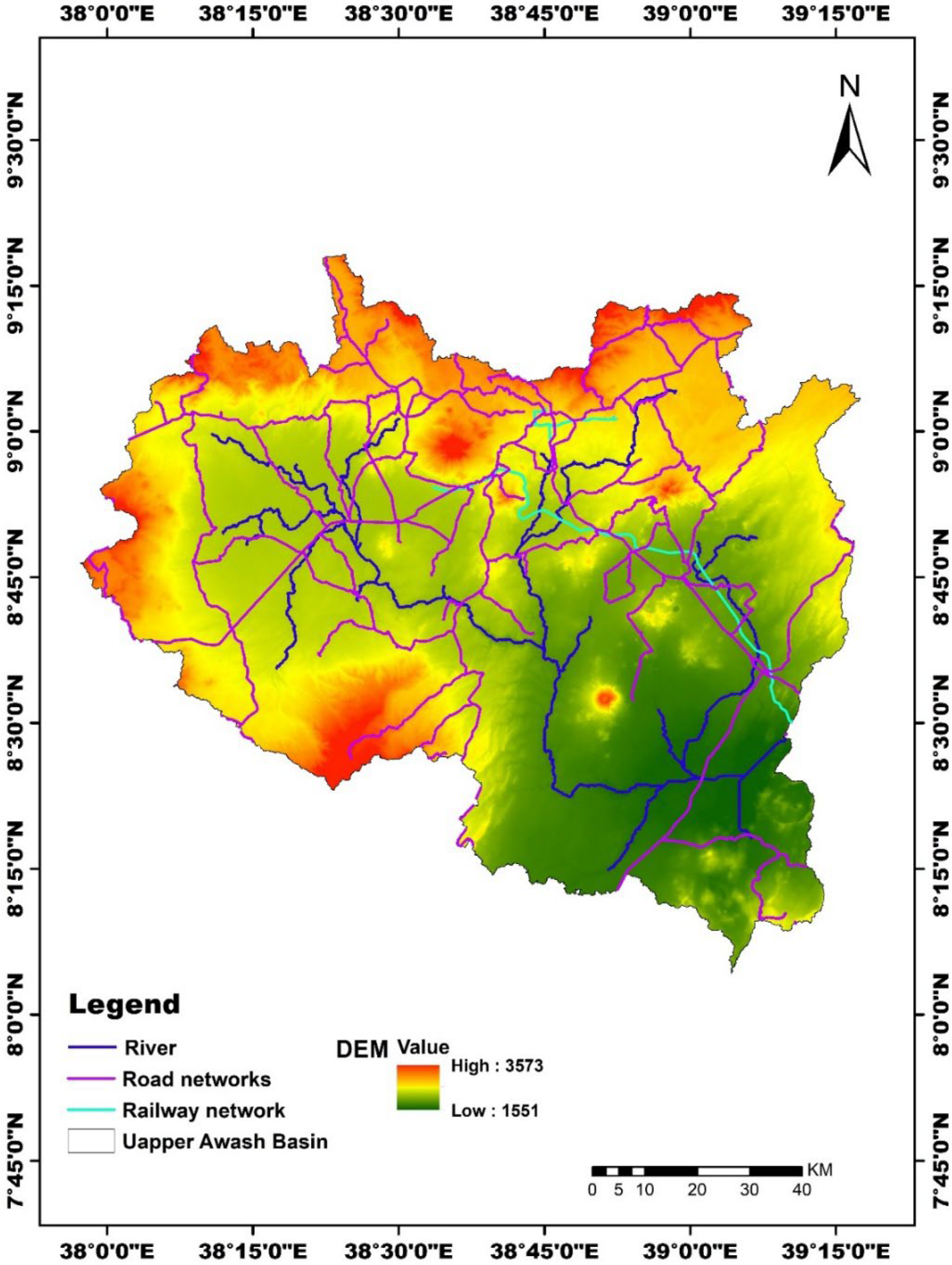
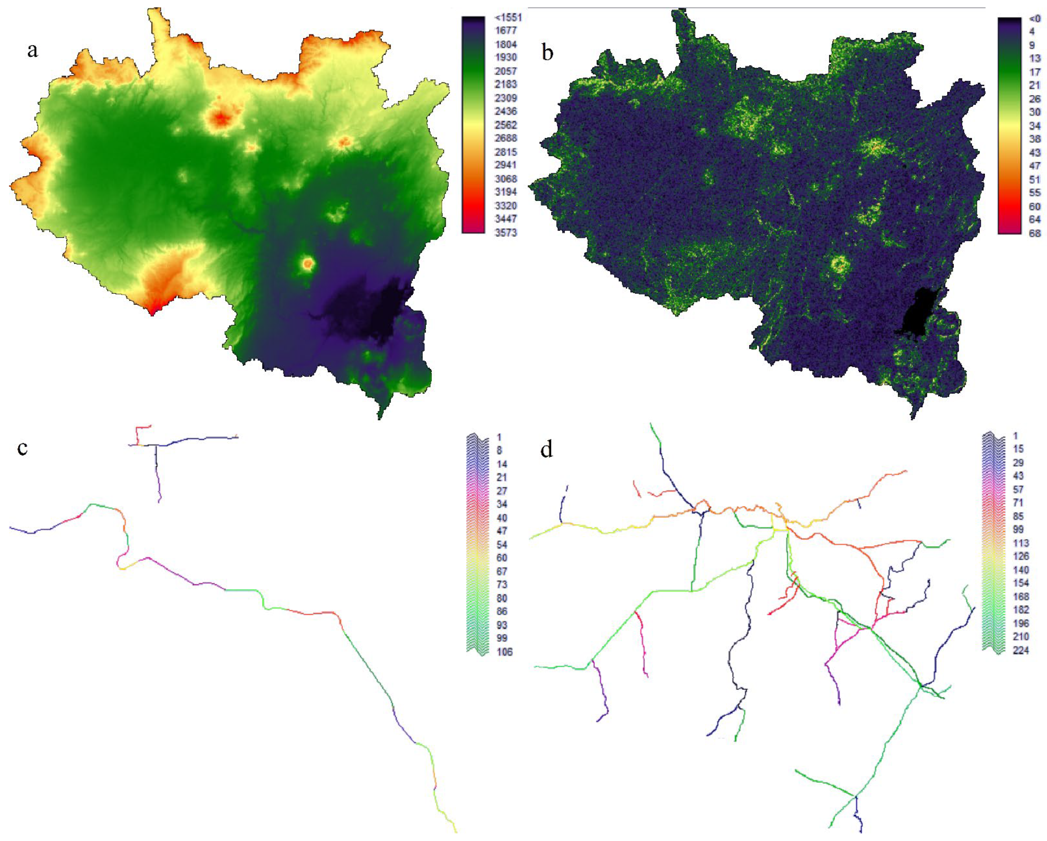
2.1. Study Area
2.2. Data Sources
2.3. Satellite Imagery Pre-Processing
2.4. LULC Classification
2.5. Accuracy Assessment
2.6. Determined Driver Factors for LUCC Prediction in the CA–Markov Model
2.7. Simulation of Future LULC Dynamics
2.8. Model Validation
2.9. Scenario-Based Projection
2.9.1. Governance (GOV)
2.9.2. Business As Usual (BAU)
3. Result
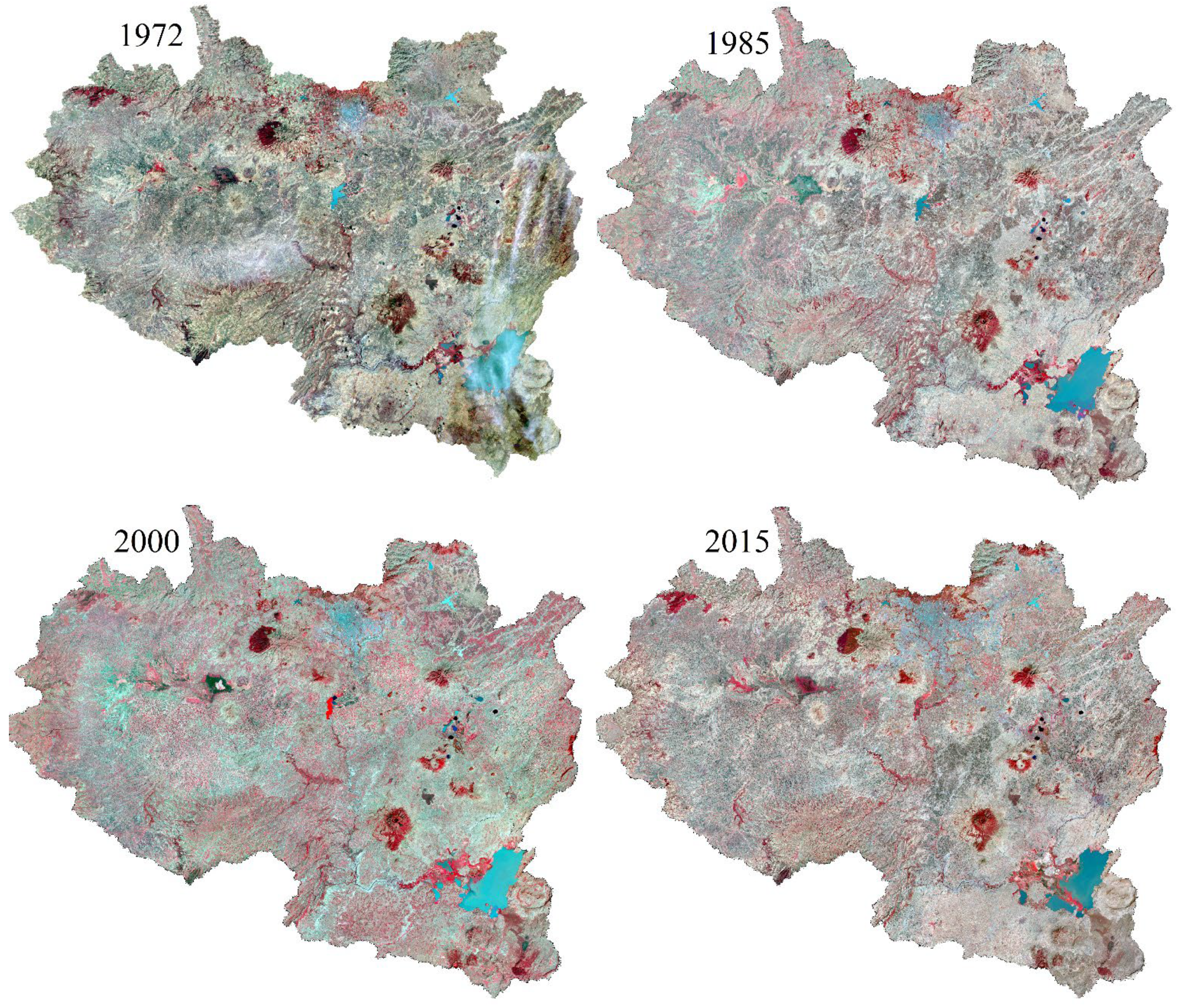
3.1. LULC Change from 1972–2015 and Accuracy Assessment
3.2. CA-Markov Model Validation
3.3. LULC Transition Probabilities Matrices
3.3.1. Conversion between 1985 and 2000
3.3.2. Conversion between 2000 and 2015
3.4. Future LULC Dynamics
4. Discussion
5. Conclusions
Author Contributions
Funding
Institutional Review Board Statement
Informed Consent Statement
Data Availability Statement
Conflicts of Interest
Appendix A


| LULC Class | Factors | Membership Function | Control Points | Constraints |
|---|---|---|---|---|
| Cropland | Slope | MD-J shape | c = 4; d = 10 | Water Urban |
| Elevation | MD-Sigmoidal | c = 2000; d =3100 | ||
| Distance from road * | MD-Sigmoidal | c = 0; d = max | ||
| Distance from railway * | MD-Sigmoidal | c = 0; d = max | ||
| Grassland | Slope | MD-J shape | c= 4; d = 10 | Water Urban |
| Elevation | MD-Sigmoidal | c = 2000; d =3100 | ||
| Distance from railway * | MD-Sigmoidal | c = 0; d = max | ||
| Distance from road * | MD-Sigmoidal | c = 0; d = max | ||
| Water | Slope | MD-J shape | c= 4; d = 10 | Urban |
| Elevation | MD-Sigmoidal | c = 2000; d =3100 | ||
| Distance from road * | MD-Sigmoidal | c = 0; d = max | ||
| Distance from railway * | MD-Sigmoidal | c = 0; d = max | ||
| Urban | Slope | MD-J shape | c = 4; d = 10 | Water |
| Elevation | MD-Sigmoidal | c = 2000; d =3100 | ||
| Distance from road * | MD-Sigmoidal | c = 0; d = max | ||
| Distance from railway * | MD-Sigmoidal | c = 0; d = max | ||
| Unused land | Slope | MD-J shape | c = 4; d = 10 | Water Urban |
| Elevation | MD-Sigmoidal | c = 2000; d =3100 | ||
| Distance from road * | MD-Sigmoidal | c = 0; d = max | ||
| Distance from railway * | MD-Sigmoidal | c = 0; d = max | ||
| Forest | Slope | MD-J shape | c = 4; d = 10 | Water Urban |
| Elevation | MD-Sigmoidal | c = 2000; d =3100 | ||
| Distance from road * | MD-Sigmoidal | c = 0; d = max | ||
| Distance from railway * | MD-Sigmoidal | c = 0; d = max | ||
| Shrubland | Slope | MD-J shape | c= 4; d = 10 | Water Urban |
| Elevation | MD-Sigmoidal | c = 2000; d =3100 | ||
| Distance from road * | MD-Sigmoidal | c = 0; d = max | ||
| Distance from railway * | MD-Sigmoidal | c = 0; d = max |
References
- Jamali, A. Evaluation and comparison of eight machine learning models in land use/land cover mapping using Landsat 8 OLI: A case study of the northern region of Iran. SN Appl. Sci. 2019, 1, 1448. [Google Scholar] [CrossRef] [Green Version]
- Palmate, S.S. Modelling spatiotemporal land dynamics for a trans-boundary river basin using integrated Cellular Automata and Markov Chain approach. Appl. Geogr. 2017, 82, 11–23. [Google Scholar] [CrossRef]
- Twisa, S.; Mwabumba, M.; Kurian, M.; Buchroithner, M. Impact of land-use/land-cover change on drinking water ecosystem services in Wami River Basin, Tanzania. Resources 2020, 9, 37. [Google Scholar] [CrossRef] [Green Version]
- Hussain, S.; Mubeen, M.; Karuppannan, S. Land use and land cover (LULC) change analysis using TM, ETM+ and OLI Landsat images in district of Okara, Punjab, Pakistan. Phys. Chem. Earth 2022, 126, 103117. [Google Scholar] [CrossRef]
- Gebresellase, S.H.; Wu, Z.; Xu, H.; Muhammad, W.I.J.T.; Climatology, A. Evaluation and selection of CMIP6 climate models in Upper Awash Basin (UBA), Ethiopia. Theor. Appl. Climatol. 2022, 149, 1521–1547. [Google Scholar] [CrossRef]
- Regasa, M.S.; Nones, M.; Adeba, D. A review on land use and land cover change in Ethiopian basins. Land 2021, 10, 585. [Google Scholar] [CrossRef]
- Hurni, H.; Tato, K.; Zeleke, G.J.M. The implications of changes in population, land use, and land management for surface runoff in the upper Nile basin area of Ethiopia. Mt. Res. Dev. 2005, 25, 147–154. [Google Scholar] [CrossRef] [Green Version]
- Zewdie, W.; Csaplovies, E. Remote sensing based multi-temporal land cover classification and change detection in northwestern Ethiopia. Eur. J. Remote Sens. 2015, 48, 121–139. [Google Scholar] [CrossRef]
- Degife, A.; Worku, H.; Gizaw, S.; Legesse, A. Land use land cover dynamics, its drivers and environmental implications in Lake Hawassa Watershed of Ethiopia. Remote Sens. Appl. Soc. Environ. 2019, 14, 178–190. [Google Scholar] [CrossRef]
- Singh, S.K.; Mustak, S.; Srivastava, P.K.; Szabó, S.; Islam, T. Predicting spatial and decadal LULC changes through cellular automata Markov chain models using earth observation datasets and geo-information. Environ. Process. 2015, 2, 61–78. [Google Scholar] [CrossRef]
- Hussain, S.; Mubeen, M.; Ahmad, A.; Majeed, H.; Qaisrani, S.A.; Hammad, H.M.; Amjad, M.; Ahmad, I.; Fahad, S.; Ahmad, N.; et al. Assessment of land use/land cover changes and its effect on land surface temperature using remote sensing techniques in Southern Punjab, Pakistan. Environ. Sci. Pollut. Res. 2022, 1–17. [Google Scholar] [CrossRef] [PubMed]
- Ul Din, S.; Mak, H. Retrieval of Land-Use/Land Cover Change (LUCC) Maps and Urban Expansion Dynamics of Hyderabad, Pakistan via Landsat Datasets and Support Vector Machine Framework. Remote Sens. 2021, 13, 3337. [Google Scholar] [CrossRef]
- Muke, M. Reported driving factors of land-use/cover changes and its mounting consequences in Ethiopia: A Review. Afr. J. Environ. Sci. Technol. 2019, 13, 273–280. [Google Scholar]
- Shi, G.; Jiang, N.; Yao, L. Land use and cover change during the rapid economic growth period from 1990 to 2010: A case study of Shanghai. Sustainability 2018, 10, 426. [Google Scholar] [CrossRef] [Green Version]
- Lambin, E.F. Modelling and monitoring land-cover change processes in tropical regions. Prog. Phys. Geogr. 1997, 21, 375–393. [Google Scholar] [CrossRef]
- Subedi, P.; Subedi, K.; Thapa, B. Application of a hybrid cellular automaton–Markov (CA-Markov) model in land-use change prediction: A case study of Saddle Creek Drainage Basin, Florida. Appl. Ecol. Environ. Sci. 2013, 1, 126–132. [Google Scholar] [CrossRef] [Green Version]
- Yang, X.; Zheng, X.-Q.; Lv, L.-N. A spatiotemporal model of land use change based on ant colony optimization, Markov chain and cellular automata. Ecol. Model. 2012, 233, 11–19. [Google Scholar] [CrossRef]
- Khoshnood Motlagh, S.; Sadoddin, A.; Haghnegahdar, A.; Razavi, S.; Salmanmahiny, A.; Ghorbani, K. Analysis and prediction of land cover changes using the land change modeler (LCM) in a semiarid river basin, Iran. Land Degrad. Dev. 2021, 32, 3092–3105. [Google Scholar] [CrossRef]
- Zhao, Q.; Li, J.; Cuan, Y.; Zhou, Z. The evolution response of ecosystem cultural services under different scenarios based on system dynamics. Remote Sens. 2020, 12, 418. [Google Scholar] [CrossRef] [Green Version]
- Gomes, E.; Inácio, M.; Bogdzevič, K.; Kalinauskas, M.; Karnauskaitė, D.; Pereira, P. Future land-use changes and its impacts on terrestrial ecosystem services: A review. Sci. Total Environ. 2021, 781, 146716. [Google Scholar] [CrossRef]
- Sun, C.; Bao, Y.; Vandansambuu, B.; Bao, Y. Simulation and Prediction of Land Use/Cover Changes Based on CLUE-S and CA-Markov Models: A Case Study of a Typical Pastoral Area in Mongolia. Sustainability 2022, 14, 15707. [Google Scholar] [CrossRef]
- Mansour, S.; Al-Belushi, M.; Al-Awadhi, T. Monitoring land use and land cover changes in the mountainous cities of Oman using GIS and CA-Markov modelling techniques. Land Use Policy 2020, 91, 104414. [Google Scholar] [CrossRef]
- Liu, X.; Ou, J.; Li, X.; Ai, B. Combining system dynamics and hybrid particle swarm optimization for land use allocation. Ecol. Model. 2013, 257, 11–24. [Google Scholar] [CrossRef]
- Guan, D.; Li, H.; Inohae, T.; Su, W.; Nagaie, T.; Hokao, K. Modeling urban land use change by the integration of cellular automaton and Markov model. Ecol. Model. 2011, 222, 3761–3772. [Google Scholar] [CrossRef]
- Islam, K.; Rahman, M.F.; Jashimuddin, M. Modeling land use change using cellular automata and artificial neural network: The case of Chunati Wildlife Sanctuary, Bangladesh. Ecol. Indic. 2018, 88, 439–453. [Google Scholar] [CrossRef]
- Halmy, M.W.A.; Gessler, P.E.; Hicke, J.A.; Salem, B.B. Land use/land cover change detection and prediction in the north-western coastal desert of Egypt using Markov-CA. Appl. Geogr. 2015, 63, 101–112. [Google Scholar] [CrossRef]
- Girma, R.; Fürst, C.; Moges, A.J. Land use land cover change modeling by integrating artificial neural network with cellular Automata-Markov chain model in Gidabo river basin, main Ethiopian rift. Environ. Chall. 2022, 6, 100419. [Google Scholar] [CrossRef]
- Daba, M.H.; You, S. Quantitatively assessing the future land-use/land-cover changes and their driving factors in the upper stream of the Awash River based on the CA–markov model and their implications for water resources management. Sustainability 2022, 14, 1538. [Google Scholar] [CrossRef]
- Munthali, M.; Mustak, S.; Adeola, A.; Botai, J.; Singh, S.; Davis, N. Modelling land use and land cover dynamics of Dedza district of Malawi using hybrid Cellular Automata and Markov model. Remote Sens. 2020, 17, 100276. [Google Scholar] [CrossRef]
- Gidey, E.; Dikinya, O.; Sebego, R.; Segosebe, E.; Zenebe, A. Cellular automata and Markov Chain (CA_Markov) model-based predictions of future land use and land cover scenarios (2015–2033) in Raya, northern Ethiopia. Model. Earth Syst. Environ. 2017, 3, 1245–1262. [Google Scholar] [CrossRef]
- Ruben, G.B.; Zhang, K.; Dong, Z.; Xia, J. Analysis and projection of land-use/land-cover dynamics through scenario-based simulations using the CA-Markov model: A case study in guanting reservoir basin, China. Sustainability 2020, 12, 3747. [Google Scholar] [CrossRef]
- Amini Parsa, V.; Yavari, A.; Nejadi, A. Spatio-temporal analysis of land use/land cover pattern changes in Arasbaran Biosphere Reserve: Iran. Model. Earth Syst. Environ. 2016, 2, 1–13. [Google Scholar] [CrossRef] [Green Version]
- Mondal, M.S.; Sharma, N.; Garg, P.K.; Kappas, M. Statistical independence test and validation of CA Markov land use land cover (LULC) prediction results. Egypt. J. Remote. Sens. Space Sci. 2016, 19, 259–272. [Google Scholar]
- Mathewos, M.; Lencha, S.M.; Tsegaye, M. Land Use and Land Cover Change Assessment and Future Predictions in the Matenchose Watershed, Rift Valley Basin, Using CA-Markov Simulation. Land 2022, 11, 1632. [Google Scholar] [CrossRef]
- Jana, A.; Jat, M.K.; Saxena, A.; Choudhary, M. Prediction of Land use land cover Changes of a river basin using the CA-Markov Model. Geocarto Int. 2022, 1–18. [Google Scholar] [CrossRef]
- Wang, J.; Bretz, M.; Dewan, M.A.A.; Delavar, M.A. Machine learning in modelling land-use and land cover-change (LULCC): Current status, challenges and prospects. Sci. Total Environ. 2022, 822, 153559. [Google Scholar] [CrossRef]
- Samie, A.; Deng, X.; Jia, S.; Chen, D. Scenario-based simulation on dynamics of land-use-land-cover change in Punjab Province, Pakistan. Sustainability 2017, 9, 1285. [Google Scholar] [CrossRef] [Green Version]
- Santé, I.; García, A.M.; Miranda, D.; Crecente, R. Cellular automata models for the simulation of real-world urban processes: A review and analysis. Landsc. Urban Plan. 2010, 96, 108–122. [Google Scholar] [CrossRef]
- Zhang, D.; Liu, X.; Wu, X.; Yao, Y.; Wu, X.; Chen, Y. Multiple intra-urban land use simulations and driving factors analysis: A case study in Huicheng, China. GIsci Remote Sens. 2019, 56, 282–308. [Google Scholar] [CrossRef]
- Keshtkar, H.; Voigt, W. A spatiotemporal analysis of landscape change using an integrated Markov chain and cellular automata models. Model. Earth Syst. Environ. 2016, 2, 10. [Google Scholar] [CrossRef] [Green Version]
- Sun, X.; Yue, T.; Fan, Z. Scenarios of changes in the spatial pattern of land use in China. Procedia Environ. Sci. 2012, 13, 590–597. [Google Scholar] [CrossRef] [Green Version]
- Peterson, G.D.; Cumming, G.S.; Carpenter, S.R. Scenario planning: A tool for conservation in an uncertain world. Conserv. Biol. 2003, 17, 358–366. [Google Scholar] [CrossRef]
- Hamad, R.; Balzter, H.; Kolo, K. Predicting land use/land cover changes using a CA-Markov model under two different scenarios. Sustainability 2018, 10, 3421. [Google Scholar] [CrossRef] [Green Version]
- Lai, Z.; Chen, C.; Chen, J.; Wu, Z.; Wang, F.; Li, S. Multi-Scenario Simulation of Land-Use Change and Delineation of Urban Growth Boundaries in County Area: A Case Study of Xinxing County, Guangdong Province. Land 2022, 11, 1598. [Google Scholar] [CrossRef]
- Biratu, A.A.; Bedadi, B.; Gebrehiwot, S.G.; Melesse, A.M.; Nebi, T.H.; Abera, W.; Tamene, L.; Egeru, A. Impact of Landscape Management Scenarios on Ecosystem Service Values in Central Ethiopia. Land 2022, 11, 1266. [Google Scholar] [CrossRef]
- Sahle, M.; Saito, O.; Fürst, C.; Demissew, S.; Yeshitela, K. Future land use management effects on ecosystem services under different scenarios in the Wabe River catchment of Gurage Mountain chain landscape, Ethiopia. Sustain. Sci. 2019, 14, 175–190. [Google Scholar] [CrossRef]
- Gebretekle, H.; Nigusse, A.G.; Demissie, B. Stream flow dynamics under current and future land cover conditions in Atsela Watershed, Northern Ethiopia. Acta Geophys. 2022, 70, 305–318. [Google Scholar] [CrossRef]
- Fikreyesus, D.; Gizaw, S.; Mayers, J.; Barrett, S. Mass Tree Planting: Prospects for a Green Legacy in Ethiopia; IIED: London, UK, 2022. [Google Scholar]
- Tiruye, G.A.; Besha, A.T.; Mekonnen, Y.S.; Benti, N.E.; Gebreslase, G.A.; Tufa, R. Opportunities and challenges of renewable energy production in Ethiopia. Sustainability 2021, 13, 10381. [Google Scholar] [CrossRef]
- Martinuzzi, S.; Radeloff, V.C.; Joppa, L.N.; Hamilton, C.M.; Helmers, D.P.; Plantinga, A.J.; Lewis, D. Scenarios of future land use change around United States’ protected areas. Biol. Conserv. 2015, 184, 446–455. [Google Scholar] [CrossRef]
- Mohamed, A.; Worku, H. Simulating urban land use and cover dynamics using cellular automata and Markov chain approach in Addis Ababa and the surrounding. Urban Clim. 2020, 31, 100545. [Google Scholar] [CrossRef]
- Peng, J.; Liu, Y.; Tian, L. Integrating ecosystem services trade-offs with paddy land-to-dry land decisions: A scenario approach in Erhai Lake Basin, southwest China. Sci. Total Environ. 2018, 625, 849–860. [Google Scholar]
- Zhang, Q.; Ban, Y.; Liu, J.; Hu, Y. Simulation and analysis of urban growth scenarios for the Greater Shanghai Area, China. Comput. Environ. Urban Syst. 2011, 35, 126–139. [Google Scholar] [CrossRef]
- Wang, R.; Hou, H.; Murayama, Y. Scenario-based simulation of Tianjin City using a cellular automata–Markov model. Sustainability 2018, 10, 2633. [Google Scholar] [CrossRef]
- Gashaw, T.; Tulu, T.; Argaw, M.; Worqlul, A.W. Evaluation and prediction of land use/land cover changes in the Andassa watershed, Blue Nile Basin, Ethiopia. Environ. Syst. Res. 2017, 6, 1–15. [Google Scholar]
- Lu, D.; Mausel, P.; Brondizio, E.; Moran, E. Change detection techniques. Int. J. Remote Sens. 2004, 25, 2365–2401. [Google Scholar] [CrossRef]
- Tadese, M.; Kumar, L.; Koech, R.; Kogo, B. Mapping of land-use/land-cover changes and its dynamics in Awash River Basin using remote sensing and GIS. Remote Sens. Appl.: Soc. Environ. 2020, 19, 100352. [Google Scholar] [CrossRef]
- Lübker, T.; Schaab, G. Identifying benefits of pre-processing large area QuickBird imagery for object-based image analysis. In Object-Based Image Analysis; Springer: Berlin/Heidelberg, Germany, 2008; pp. 203–219. [Google Scholar]
- Sowmya, D.; Deepa Shenoy, P.; Venugopal, K. Remote sensing satellite image processing techniques for image classification: A comprehensive survey. Int. J. Comput. Appl. 2017, 161, 24–37. [Google Scholar]
- Nalluri, A.; Ramesh, H. A comparative study of radiometric corrections on multispectral and panchromatic images. Asian J. Converg. Technol. (AJCT) 2019. [Google Scholar]
- Mohamed, M.R. Estimating Salinity Using Remote Sensing Data. J. Al-Azhar Univ. Eng. Sect. 2022, 17, 1143–1156. [Google Scholar]
- Mehmood, M.; Shahzad, A.; Zafar, B.; Shabbir, A.; Ali, N. Remote sensing image classification: A comprehensive review and applications. Math. Probl. Eng. 2022, 2022, 5880959. [Google Scholar] [CrossRef]
- Shawul, A.A.; Chakma, S. Spatiotemporal detection of land use/land cover change in the large basin using integrated approaches of remote sensing and GIS in the Upper Awash basin, Ethiopia. Environ. Earth Sci. 2019, 78, 141. [Google Scholar] [CrossRef]
- Wang, J.; Yang, M.; Chen, Z.; Lu, J.; Zhang, L. An MLC and U-Net Integrated Method for Land Use/Land Cover Change Detection Based on Time Series NDVI-Composed Image from PlanetScope Satellite. Water 2022, 14, 3363. [Google Scholar] [CrossRef]
- Hord, R.M. Digital Image Processing of Remotely Sensed Data; Elsevier: Amsterdam, The Netherlands, 1982. [Google Scholar]
- Kostovska, A.; Doerr, C.; Džeroski, S.; Kocev, D.; Panov, P.; Eftimov, T. Explainable Model-specific Algorithm Selection for Multi-Label Classification. arXiv 2022, arXiv:2211.11227. [Google Scholar]
- Wang, S.W.; Munkhnasan, L.; Lee, W.-K. Land use and land cover change detection and prediction in Bhutan’s high altitude city of Thimphu, using cellular automata and Markov chain. Environ. Chall. 2021, 2, 100017. [Google Scholar] [CrossRef]
- Foody, G.M. Status of land cover classification accuracy assessment. Remote Sens. Environ. 2002, 80, 185–201. [Google Scholar] [CrossRef]
- Manandhar, R.; Odeh, I.O.; Ancev, T. Improving the accuracy of land use and land cover classification of Landsat data using post-classification enhancement. Remote Sens. 2009, 1, 330–344. [Google Scholar] [CrossRef] [Green Version]
- Congalton, R.G. A review of assessing the accuracy of classifications of remotely sensed data. Remote Sens. Environ. 1991, 37, 35–46. [Google Scholar] [CrossRef]
- Cracknell, A.P. Introduction to Remote Sensing; CRC Press: Boca Raton, FL, USA, 2007. [Google Scholar]
- Liu, C.; Frazier, P.; Kumar, L. Comparative assessment of the measures of thematic classification accuracy. Remote Sens. Environ. 2007, 107, 606–616. [Google Scholar] [CrossRef]
- Ikiel, C.; Dutucu, A.A.; Ustaoglu, B.; Kilic, D.E. Land use and land cover (LULC) classification using Spot-5 image in the Adapazari Plain and its surroundings, Turkey. J. Sci. Technol. 2012, 2, 37–42. [Google Scholar]
- Zanotta, D.C.; Zortea, M.; Ferreira, M. A supervised approach for simultaneous segmentation and classification of remote sensing images. ISPRS J. Photogramm. Remote Sens. 2018, 142, 162–173. [Google Scholar]
- Congalton, R.G. Thematic and positional accuracy assessment of digital remotely sensed data. In Proceedings of the Seventh Annual Forest Inventory and Analysis Symposium, Portland, OR, USA, 3-6 October 2005; General Technical Report WO; McRoberts, R.E., Reams, G.A., Van Deusen, P.C., McWilliams, W.H., Eds.; US Department of Agriculture, Forest Service: Washington, DC, USA, 2007; pp. 149–154. [Google Scholar]
- Richards, J.A.; Richards, J. Remote Sensing Digital Image Analysis; Springer: Berlin/Heidelberg, Germany, 1999; Volume 3. [Google Scholar]
- Story, M.; Congalton, R.G. Accuracy assessment: A user’s perspective. Photogramm. Eng. Remote Sens. 1986, 52, 397–399. [Google Scholar]
- Woldesenbet, T.A.; Elagib, N.A.; Ribbe, L.; Heinrich, J.J. Catchment response to climate and land use changes in the Upper Blue Nile sub-basins, Ethiopia. Sci. Total Environ. 2018, 644, 193–206. [Google Scholar] [CrossRef] [PubMed]
- Gebrechorkos, S.H.; Bernhofer, C.; Hülsmann, S. Climate change impact assessment on the hydrology of a large river basin in Ethiopia using a local-scale climate modelling approach. Sci. Total Environ. 2020, 742, 140504. [Google Scholar] [CrossRef] [PubMed]
- Mas, J.-F.; Kolb, M.; Paegelow, M.; Olmedo, M.T.C.; Houet, T. Inductive pattern-based land use/cover change models: A comparison of four software packages. Environ. Model. Softw. 2014, 51, 94–111. [Google Scholar] [CrossRef] [Green Version]
- Marhaento, H.; Booij, M.J.; Hoekstra, A. Hydrological response to future land-use change and climate change in a tropical catchment. Hydrol. Sci. J. 2018, 63, 1368–1385. [Google Scholar] [CrossRef] [Green Version]
- Hyandye, C.; Mandara, C.G.; Safari, J. GIS and logit regression model applications in land use/land cover change and distribution in Usangu catchment. J. Remote Sens. Technol. 2015, 3, 149–154. [Google Scholar] [CrossRef] [Green Version]
- Azizi, P.; Soltani, A.; Bagheri, F.; Sharifi, S.; Mikaeili, M. An Integrated Modelling Approach to Urban Growth and Land Use/Cover Change. Land 2022, 11, 1715. [Google Scholar] [CrossRef]
- Ghafoor, G.Z.; Sharif, F.; Shahid, M.G.; Shahzad, L.; Rasheed, R.; Khan, A.U.H. Assessing the impact of land use land cover change on regulatory ecosystem services of subtropical scrub forest, Soan Valley Pakistan. Sci. Rep. 2022, 12, 10052. [Google Scholar] [CrossRef]
- López, E.; Bocco, G.; Mendoza, M.; Duhau, E. Predicting land-cover and land-use change in the urban fringe: A case in Morelia city, Mexico. Landsc. Urban Plan. 2001, 55, 271–285. [Google Scholar] [CrossRef]
- Al-sharif, A.A.; Pradhan, B. Monitoring and predicting land use change in Tripoli Metropolitan City using an integrated Markov chain and cellular automata models in GIS. Arab. J. Geosci. 2014, 7, 4291–4301. [Google Scholar] [CrossRef]
- Muller, M.R.; Middleton, J. A Markov model of land-use change dynamics in the Niagara Region, Ontario, Canada. Landsc. Ecol. 1994, 9, 151–157. [Google Scholar]
- Yangouliba, G.I.; Zoungrana, B.J.-B.; Hackman, K.O.; Koch, H.; Liersch, S.; Sintondji, L.O.; Dipama, J.-M.; Kwawuvi, D.; Ouedraogo, V.; Yabré, S.; et al. Modelling past and future land use and land cover dynamics in the Nakambe River Basin, West Africa. Model. Earth Syst. Environ. 2022, 1–17. [Google Scholar] [CrossRef]
- Memarian, H.; Balasundram, S.K.; Talib, J.B.; Sung, C.T.B.; Sood, A.M.; Abbaspour, K. Validation of CA-Markov for simulation of land use and cover change in the Langat Basin, Malaysia. J. Geogr. Inf. Syst. 2012, 4, 26322. [Google Scholar] [CrossRef] [Green Version]
- Tontisirin, N.; Anantsuksomsri, S. Economic development policies and land use changes in Thailand: From the eastern seaboard to the eastern economic corridor. Sustainability 2021, 13, 6153. [Google Scholar] [CrossRef]
- Wang, M.; Cai, L.; Xu, H.; Zhao, S. Predicting land use changes in northern China using logistic regression, cellular automata, and a Markov model. Arab. J. Geosci. 2019, 12, 790. [Google Scholar] [CrossRef]
- Omar, N.; Sanusi, S.; Hussin, W.; Samat, N.; Mohammed, K.S. Markov-CA model using analytical hierarchy process and multiregression technique. In IOP Conference Series: Earth and Environmental Science; IOP Publishing: Bristol, UK, 2020; Volume 20, p. 012008. [Google Scholar]
- Malczewski, J. GIS-based multicriteria decision analysis: A survey of the literature. Int. J. Geogr. Inf. Sci. 2006, 20, 703–726. [Google Scholar] [CrossRef]
- Malczewski, J. On the use of weighted linear combination method in GIS: Common and best practice approaches. Trans GIS. 2000, 4, 5–22. [Google Scholar] [CrossRef]
- Saaty, T.L. Decision making with the analytic hierarchy process. Int. J. Serv. Sci. 2008, 1, 83–98. [Google Scholar] [CrossRef] [Green Version]
- Palmate, S.S.; Wagner, P.D.; Fohrer, N.; Pandey, A. Assessment of Uncertainties in Modelling Land Use Change with an Integrated Cellular Automata–Markov Chain Model. Environ. Model. Assess. 2022, 27, 275–293. [Google Scholar] [CrossRef]
- Clarke, K.C.; Gaydos, L.J. Loose-coupling a cellular automaton model and GIS: Long-term urban growth prediction for San Francisco and Washington/Baltimore. Int J Geogr Inf Sci. 1998, 12, 699–714. [Google Scholar] [CrossRef] [Green Version]
- García-Álvarez, D.; Camacho Olmedo, M.T.; Paegelow, M.; Mas, J.F. Land Use Cover Datasets and Validation Tools: Validation Practices with QGIS; Springer: Berlin/Heidelberg, Germany, 2022. [Google Scholar]
- Singh, A.K. Modelling Land Use Land Cover Changes Using Cellular Automata in a Geo-Spatial Environment. Master’s thesis, ITC, Enschede, The Netherlands, 2003. [Google Scholar]
- Alemu, B.; Garedew, E.; Eshetu, Z.; Kassa, H. Land use and land cover changes and associated driving forces in north western lowlands of Ethiopia. Int. Res. J. Agric. Sci. Soil Sci. 2015, 5, 28–44. [Google Scholar]
- Ayana, A.B.; Kositsakulchai, E.J.A.; Resources, N. Land use change analysis using remote sensing and Markov Modeling in Fincha watershed, Ethiopia. Agric. Nat. Resour. 2012, 46, 135–149. [Google Scholar]
- Mohammed, M.; Habtamu, T.; Yared, M. Land use/cover change analysis and local community perception towards land cover change in the lowland of Bale rangelands, Southeast Ethiopia. Int. J. Biodivers. Conserv. 2017, 9, 363–372. [Google Scholar] [CrossRef] [Green Version]
- Bewket, W. Land cover dynamics since the 1950s in Chemoga watershed, Blue Nile basin, Ethiopia. Mt. Res. Dev. 2002, 22, 263–269. [Google Scholar] [CrossRef]
- Tekle, K.; Hedlund, L. Land cover changes between 1958 and 1986 in Kalu District, southern Wello, Ethiopia. Mt. Res Dev. 2000, 20, 42–51. [Google Scholar] [CrossRef] [Green Version]
- Atsbha, T.; Desta, A.B.; Zewdu, T. Carbon sequestration potential of natural vegetation under grazing influence in Southern Tigray, Ethiopia: Implication for climate change mitigation. Heliyon 2019, 5, e02329. [Google Scholar] [CrossRef] [PubMed] [Green Version]
- Giriraj, A.; Irfan-Ullah, M.; Murthy, M.S.R.; Beierkuhnlein, C. Modelling spatial and temporal forest cover change patterns (1973-2020): A case study from South Western Ghats (India). Sensors 2008, 8, 6132–6153. [Google Scholar] [CrossRef] [PubMed] [Green Version]
- Adhikari, S.; Southworth, J. Simulating forest cover changes of Bannerghatta National Park based on a CA-Markov model: A remote sensing approach. Remote Sens. 2012, 4, 3215–3243. [Google Scholar] [CrossRef] [Green Version]
- Godebo, T.R.; Jeuland, M.A.; Paul, C.J.; Belachew, D.L.; McCornick, P.G. Water quality threats, perceptions of climate change and behavioral responses among farmers in the Ethiopian Rift Valley. Climate 2021, 9, 92. [Google Scholar] [CrossRef]
- Gelibo, T.; Lulseged, S.; Eshetu, F.; Abdella, S.; Melaku, Z.; Ajiboye, S.; Demissie, M.; Solmo, C.; Ahmed, J.; Getaneh, Y. Spatial distribution and determinants of HIV prevalence among adults in urban Ethiopia: Findings from the Ethiopia Population-based HIV Impact Assessment Survey (2017–2018). PLoS ONE 2022, 17, e0271221. [Google Scholar] [CrossRef]
- Fung, T.; LeDrew, E.J.P. For change detection using various accuracy. Photogramm. Eng. Remote Sens. 1988, 54, 1449–1454. [Google Scholar]


| Satellite/Sensor | Acquisition date | Path | Row | Spatial Resolution (m) |
|---|---|---|---|---|
| Landsat 1 MSS | 31 January 1972 | 181 | 54 | 60 |
| 30 January 1972 | 180 | 54 | 60 | |
| Landsat 5 TM | 22 November 1985 | 169 | 54 | 30 |
| 21 January 1985 | 168 | 54 | 30 | |
| Landsat 7 ETM+ | 26 November 2000 | 169 | 54 | 15 |
| 5 December 2000 | 168 | 54 | 15 | |
| Landsat 8 OLI TIRS | 20 December 2015 | 168 | 54 | 30 |
| 28 January 2015 | 169 | 54 | 30 |
| LULC Classes | Description |
|---|---|
| Urban | Urbanized areas and rural settlements |
| Water | A stream or river, a lake, a pond or a reservoir |
| Cropland | A plot of land used to grow a variety of crops |
| Shrubland | Chaparrals, woodlands, and savannas |
| Forest | Dense trees |
| Grassland | Dense grass, moderate grass, and sparse grass |
| Unused land | Terrains with loose, eroded, or bare soils |
| LULC | 1972 | 1985 | 2000 | 2015 | ||||
|---|---|---|---|---|---|---|---|---|
| Area (km2) | Area (%) | Area (km2) | Area (%) | Area (km2) | Area (%) | Area (km2) | Area (%) | |
| Urban | 52.53 | 0.45 | 90.62 | 0.77 | 173.86 | 1.48 | 354.14 | 3.01 |
| Water | 204.87 | 1.74 | 192.81 | 1.64 | 188.05 | 1.60 | 152.44 | 1.29 |
| Cropland | 6040.75 | 51.25 | 7634.33 | 64.94 | 7937.15 | 67.52 | 8472.45 | 71.97 |
| Shrubland | 2462.99 | 20.89 | 1939.41 | 16.50 | 2350.42 | 19.99 | 1399.49 | 11.89 |
| Forest | 834.67 | 7.08 | 801.93 | 6.82 | 500.00 | 4.25 | 875.46 | 7.44 |
| Grassland | 2052.08 | 17.41 | 986.89 | 8.39 | 441.63 | 3.76 | 447.63 | 3.80 |
| Unused land | 139.95 | 1.19 | 109.75 | 0.93 | 164.64 | 1.40 | 70.28 | 0.60 |
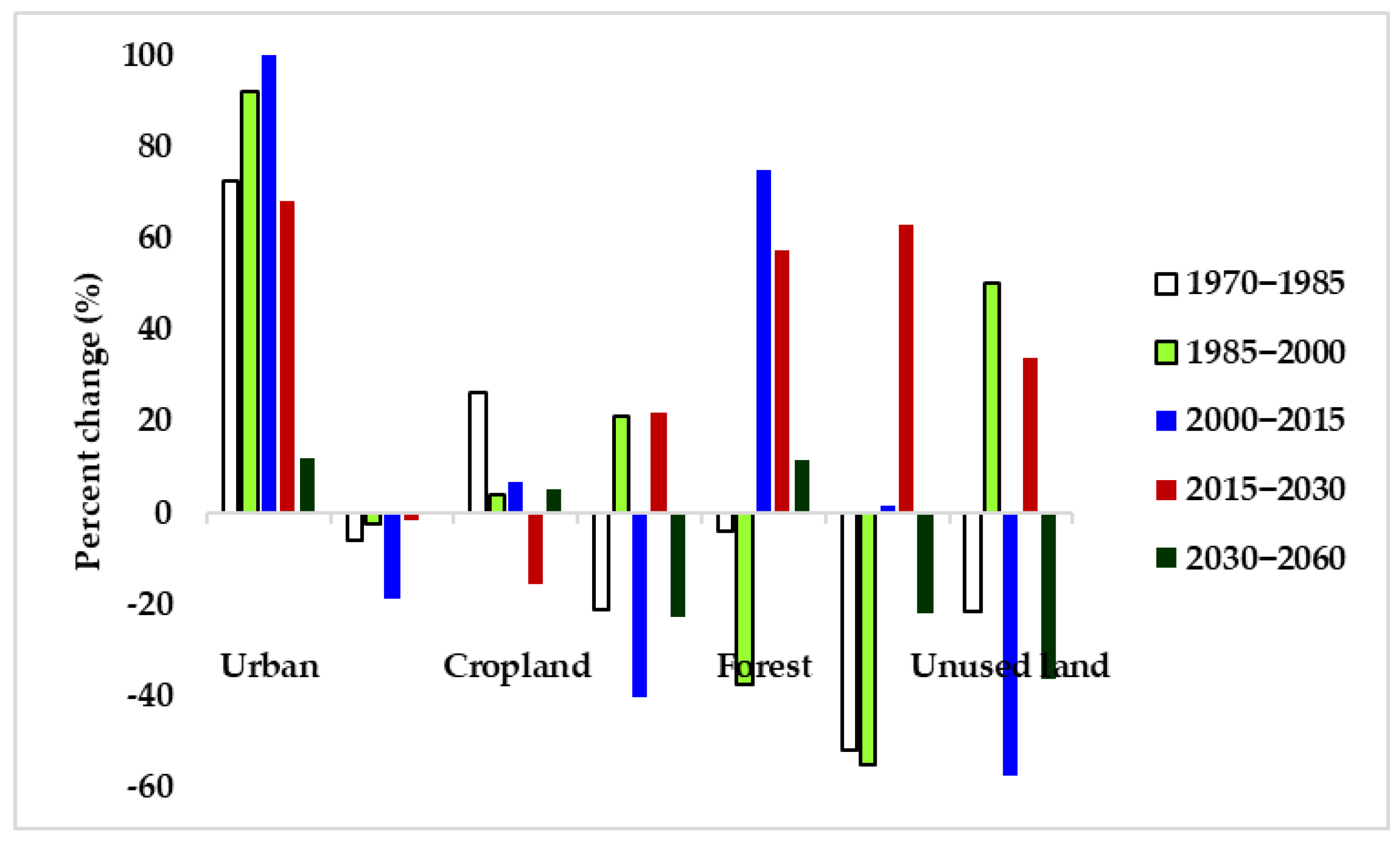
| LULC | 1972–1985 | 1985–2000 | 2000–2015 | 1972–2015 |
|---|---|---|---|---|
| Urban | +72.52 | +91.86 | +103.69 | +574.17 |
| Water | −5.88 | −2.47 | −18.94 | −25.59 |
| Cropland | +26.38 | +3.97 | +6.74 | +40.25 |
| Shrubland | −21.26 | +21.19 | −40.46 | −43.18 |
| Forest | −3.92 | −37.65 | +75.09 | +4.89 |
| Grassland | −51.91 | −55.25 | +1.36 | −78.19 |
| Unused land | −21.58 | +50.01 | −57.31 | −49.78 |
| LULC 1972 | LULC 1985 | LULC 2000 | LULC 2015 | |||||
|---|---|---|---|---|---|---|---|---|
| LULC Class | UA | PA | UA | PA | UA | PA | UA | PA |
| Urban | 75.2 | 74.7 | 90.0 | 87.9 | 96.5 | 85 | 93.4 | 92.7 |
| Water | 80.5 | 80.5 | 95 | 91.0 | 100.0 | 92.13 | 100.0 | 100.0 |
| Cropland | 76.5 | 86.6 | 78.5 | 88.7 | 65.67 | 88 | 82.3 | 97.6 |
| Shrubland | 75.0 | 75.0 | 75.6 | 87.7 | 79.09 | 87.88 | 97.1 | 77 |
| Forest | 90.4 | 77.7 | 90.1 | 87.4 | 98.9 | 90.88 | 88.0 | 86.8 |
| Grassland | 70.9 | 85.6 | 82.0 | 91.8 | 98.9 | 93.07 | 82.1 | 78.6 |
| Unused land | 76.2 | 72.7 | 96.7 | 88.9 | 96.9 | 90 | 94.3 | 91.9 |
| Overall accuracy | 80.6 | 89.04 | 89.41 | 89.2 | ||||
| Kappa coefficient | 0.76 | 0.87 | 0.87 | 0.87 | ||||
| Kappa Index | Kappa Index of Agreement (%) |
|---|---|
| Kno | 90 |
| K-standard | 87 |
| K-locality | 92 |
| LULC Category | KIA 1 | LULC Category | KIA |
|---|---|---|---|
| Urban | 0.83 | Forest | 0.82 |
| Water | 0.93 | Grassland | 0.80 |
| Cropland | 0.81 | Unused land | 0.71 |
| Shrubland | 0.74 | ||
| Overall KIA | 0.87 |
| LULC Category | Actual Map of 2015 | Simulated Map of 2015 | ||
|---|---|---|---|---|
| km2 | % | km2 | % | |
| Urban | 354.14 | 3.01 | 511.14 | 4.34 |
| Water | 152.44 | 1.29 | 145.12 | 1.23 |
| Cropland | 8472.45 | 71.97 | 7835.64 | 66.50 |
| Shrubland | 1399.49 | 11.89 | 1628.41 | 13.82 |
| Forest | 875.46 | 7.44 | 1080.85 | 9.17 |
| Grassland | 447.63 | 3.80 | 498.30 | 4.23 |
| Unused land | 70.28 | 0.60 | 83.01 | 0.70 |
| 1985 | 2000 | ||||||
|---|---|---|---|---|---|---|---|
| Urban | Water | Cropland | Shrubland | Forest | Grassland | Unused Land | |
| Urban | 0.6992 | 0.0081 | 0.1117 | 0.0846 | 0.0835 | 0.0083 | 0.0047 |
| Water | 0.0125 | 0.7691 | 0.0879 | 0.0910 | 0.0322 | 0.0000 | 0.0072 |
| Cropland | 0.0097 | 0.0006 | 0.6693 | 0.2034 | 0.0572 | 0.0337 | 0.0260 |
| Shrubland | 0.0197 | 0.0041 | 0. 5736 | 0.2924 | 0.0382 | 0.0640 | 0.0079 |
| Forest | 0.0073 | 0.0033 | 0.2859 | 0.4671 | 0.1430 | 0.0847 | 0.0089 |
| Grassland | 0.0081 | 0.0004 | 0.5887 | 0.3067 | 0.0086 | 0.0814 | 0.0061 |
| Unused land | 0.0164 | 0.0005 | 0.8003 | 0.1088 | 0.0033 | 0.0021 | 0.0686 |
| 2000 | 2015 | ||||||
|---|---|---|---|---|---|---|---|
| Urban | Water | Cropland | Shrubland | Forest | Grassland | Unused Land | |
| Urban | 0.5991 | 0.0082 | 0.1409 | 0.1196 | 0.0922 | 0.0387 | 0.0013 |
| Water | 0.0022 | 0.6387 | 0.1421 | 0.1180 | 0.0946 | 0.0043 | 0.0002 |
| Cropland | 0.0394 | 0.0011 | 0.7021 | 0.1477 | 0.0664 | 0.0338 | 0.0096 |
| Shrubland | 0.0130 | 0.0016 | 0. 5462 | 0.1998 | 0.1619 | 0.0759 | 0.0016 |
| Forest | 0.0312 | 0.0016 | 0.6269 | 0.0859 | 0.2412 | 0.0118 | 0.0014 |
| Grassland | 0.0083 | 0.0001 | 0.5243 | 0.1895 | 0.0754 | 0.2020 | 0.0005 |
| Unused land | 0.0083 | 0.0051 | 0.7790 | 0.0523 | 0.0308 | 0.0175 | 0.1069 |
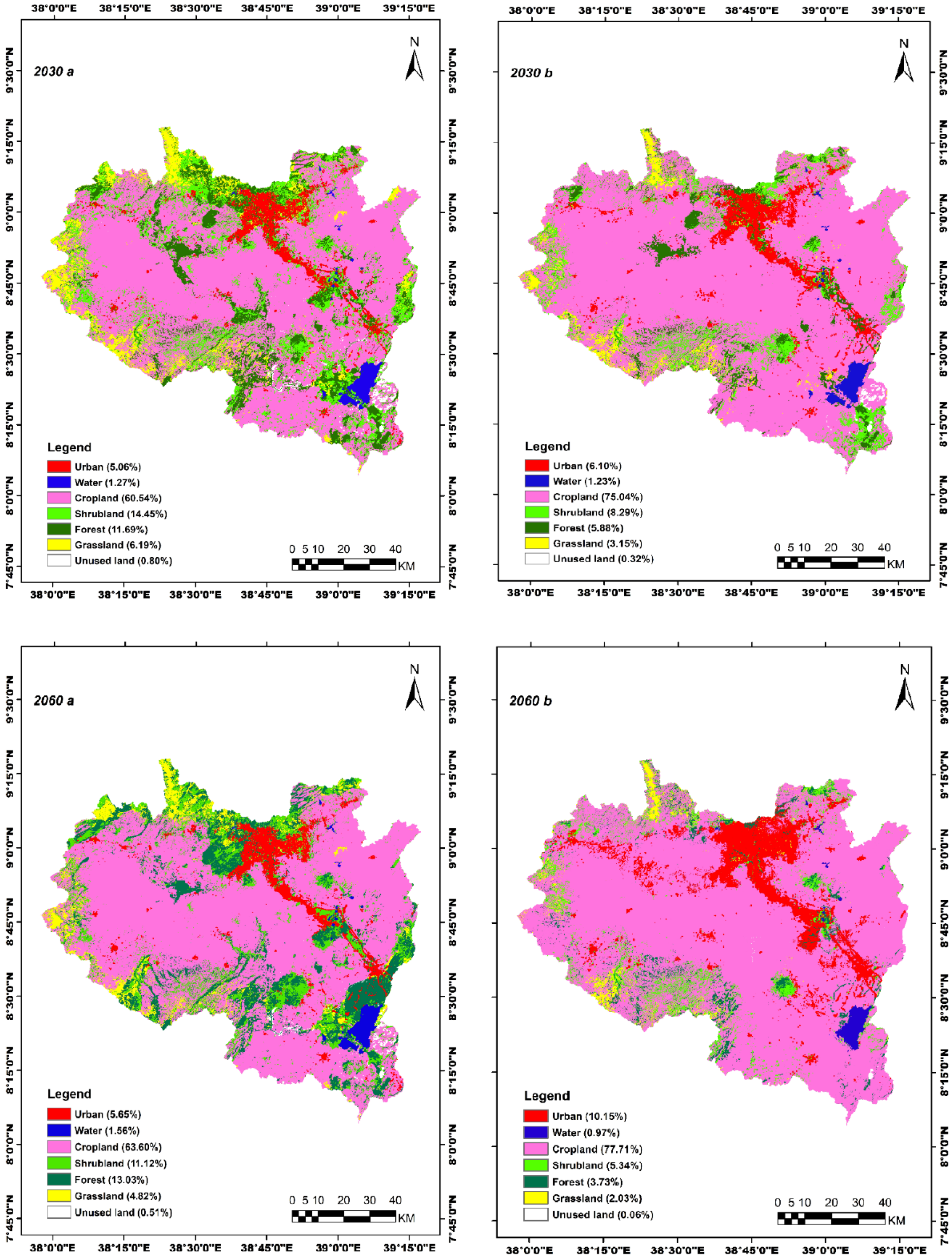
| LULC Category | Reference | BAU | Gov | |||||||
|---|---|---|---|---|---|---|---|---|---|---|
| 2015 | 2030 | 2060 | 2030 | 2060 | ||||||
| km2 | % | km2 | % | km2 | % | km2 | % | km2 | % | |
| Urban | 354.14 | 3.01 | 717.67 | 6.1 | 1196.78 | 10.15 | 595.78 | 5.06 | 665.80 | 5.65 |
| Water | 152.44 | 1.29 | 144.38 | 1.23 | 114.83 | 0.97 | 149.88 | 1.27 | 149.78 | 1.56 |
| Cropland | 8472.45 | 71.97 | 8833.65 | 75.04 | 9159.21 | 77.71 | 7134.88 | 60.54 | 7500.90 | 63.6 |
| Shrubland | 1399.49 | 11.89 | 976.42 | 8.29 | 629.61 | 5.34 | 1703.06 | 14.45 | 1312.03 | 11.12 |
| Forest | 875.46 | 7.44 | 692.21 | 5.88 | 439.95 | 3.73 | 1378.15 | 11.69 | 1537.19 | 13.03 |
| Grassland | 447.63 | 3.8 | 370.24 | 3.15 | 239.58 | 2.03 | 729.66 | 6.19 | 568.35 | 4.82 |
| Unused land | 70.28 | 0.6 | 37.13 | 0.32 | 6.73 | 0.06 | 94.01 | 0.8 | 59.72 | 0.51 |
Disclaimer/Publisher’s Note: The statements, opinions and data contained in all publications are solely those of the individual author(s) and contributor(s) and not of MDPI and/or the editor(s). MDPI and/or the editor(s) disclaim responsibility for any injury to people or property resulting from any ideas, methods, instructions or products referred to in the content. |
© 2023 by the authors. Licensee MDPI, Basel, Switzerland. This article is an open access article distributed under the terms and conditions of the Creative Commons Attribution (CC BY) license (https://creativecommons.org/licenses/by/4.0/).
Share and Cite
Gebresellase, S.H.; Wu, Z.; Xu, H.; Muhammad, W.I. Scenario-Based LULC Dynamics Projection Using the CA–Markov Model on Upper Awash Basin (UAB), Ethiopia. Sustainability 2023, 15, 1683. https://doi.org/10.3390/su15021683
Gebresellase SH, Wu Z, Xu H, Muhammad WI. Scenario-Based LULC Dynamics Projection Using the CA–Markov Model on Upper Awash Basin (UAB), Ethiopia. Sustainability. 2023; 15(2):1683. https://doi.org/10.3390/su15021683
Chicago/Turabian StyleGebresellase, Selamawit Haftu, Zhiyong Wu, Huating Xu, and Wada Idris Muhammad. 2023. "Scenario-Based LULC Dynamics Projection Using the CA–Markov Model on Upper Awash Basin (UAB), Ethiopia" Sustainability 15, no. 2: 1683. https://doi.org/10.3390/su15021683