
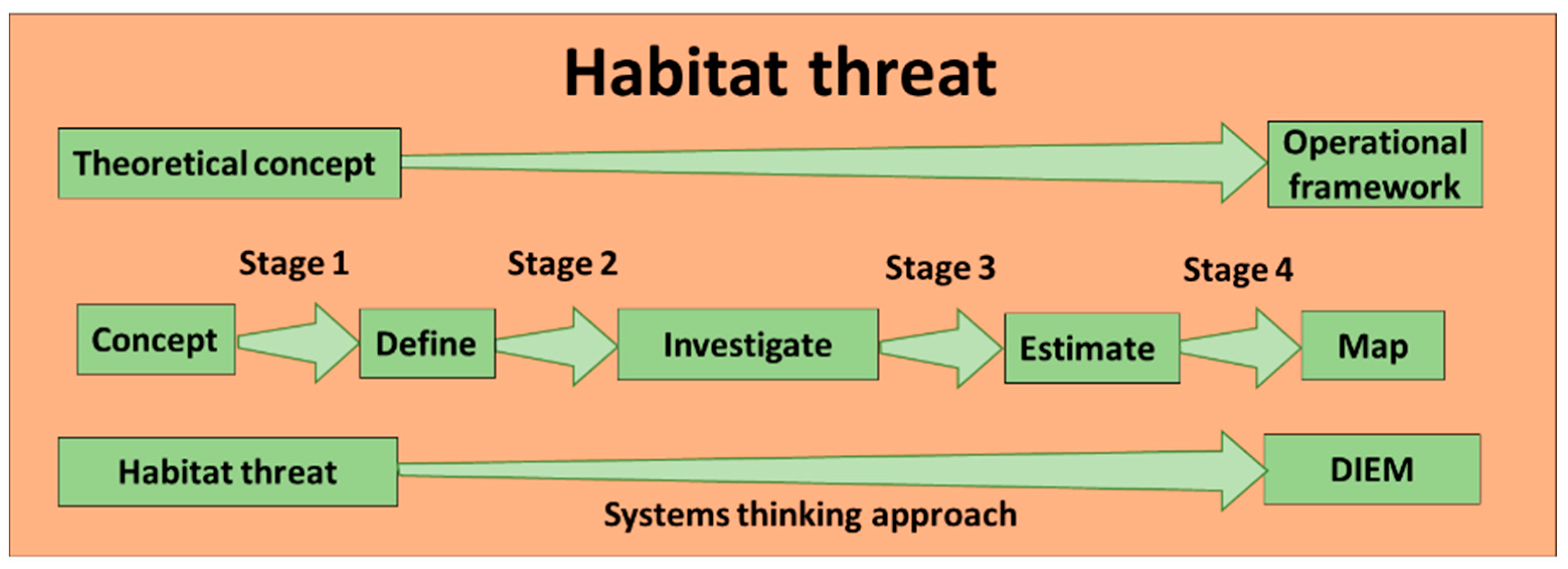
Define–Investigate–Estimate–Map (DIEM) Framework for Modeling Habitat Threats


Abstract
:1. Introduction
2. Materials and Methods
2.1. Meta-Analysis
- A document search was performed using Google Scholar on 26 November 2019. The keywords “threat index” and “habitat threat” were used, which gave 3370 results and 406 results, respectively, for a total of 3776 articles. The search range of years was set as 2000–2019 to capture the past two decades. Out of the 3776 retrieved articles, 401 were identified as being related to habitat threats. The selection criteria for determining whether an article was relevant were accessibility and context. Full-text articles available for viewing and downloading were included. Articles pertaining to threat indices such as political, sports, personal health, and vehicular threats were excluded.
- The article pool was then further narrowed by selecting articles that fit the criteria of describing environmental, ecological, biodiversity, and habitat threats. We retrieved 34 references that had been published between 2003 and 2019.
- Forward and backward snowball sampling was utilized in these 34 papers. These processes involve analyzing papers that cite a previously retrieved paper (forwards) and reviewing papers that the retrieved paper cited (backwards). An additional 28 relevant papers were found that were not in the initial set of search results. The total number of papers increased to 62. These papers were published between 1997 and 2019.
- These 62 papers were analyzed by gathering information pertaining to the definitions, types, and characteristics of habitat threats. Of the 62 papers, 24 articles were used to define habitat threat, 44 articles were used to synthesize the types of threat, 11 articles were used to synthesize threat characteristics, and 14 articles were used to understand threat index calculations. Several articles provided information on multiple subjects.
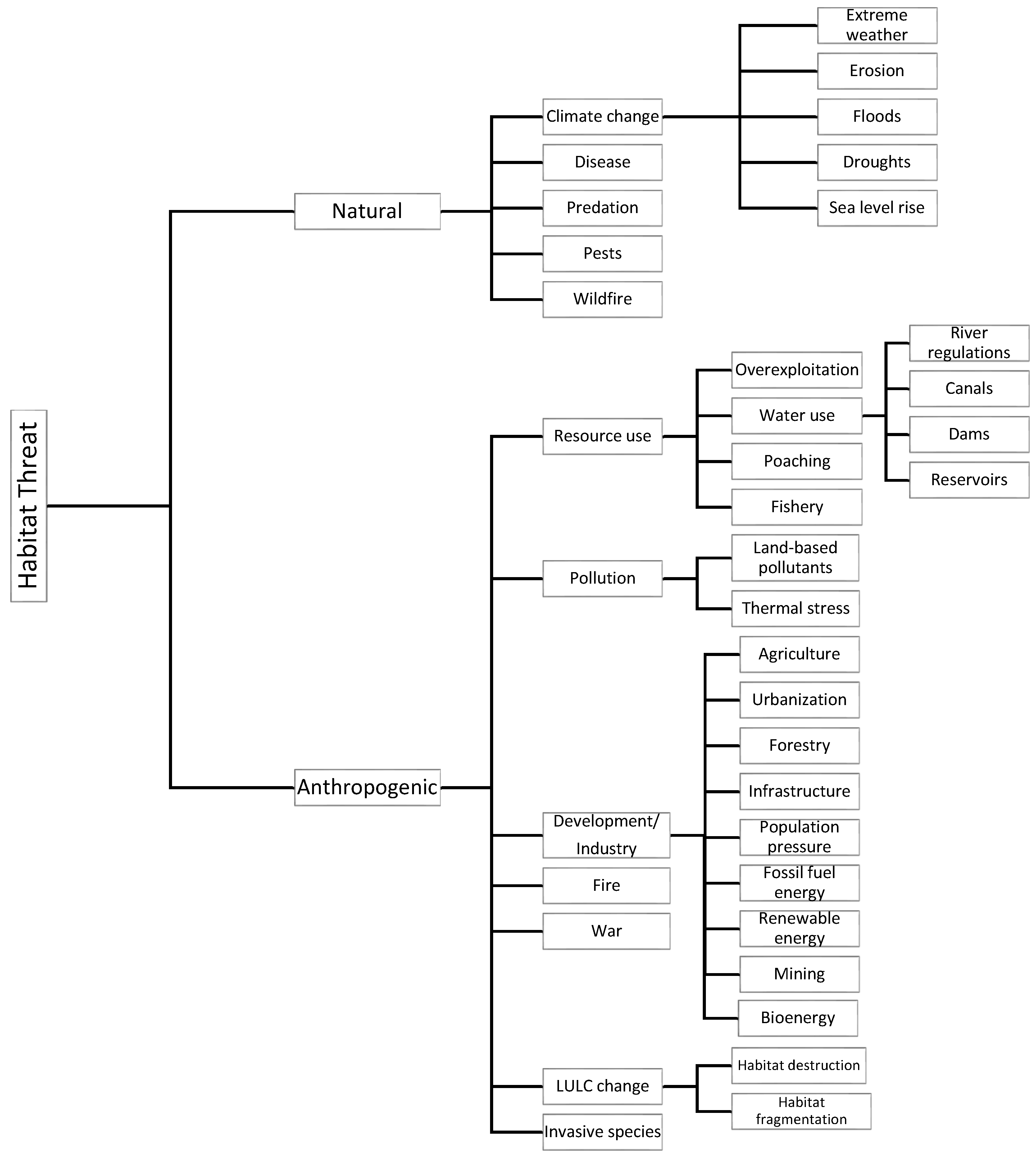
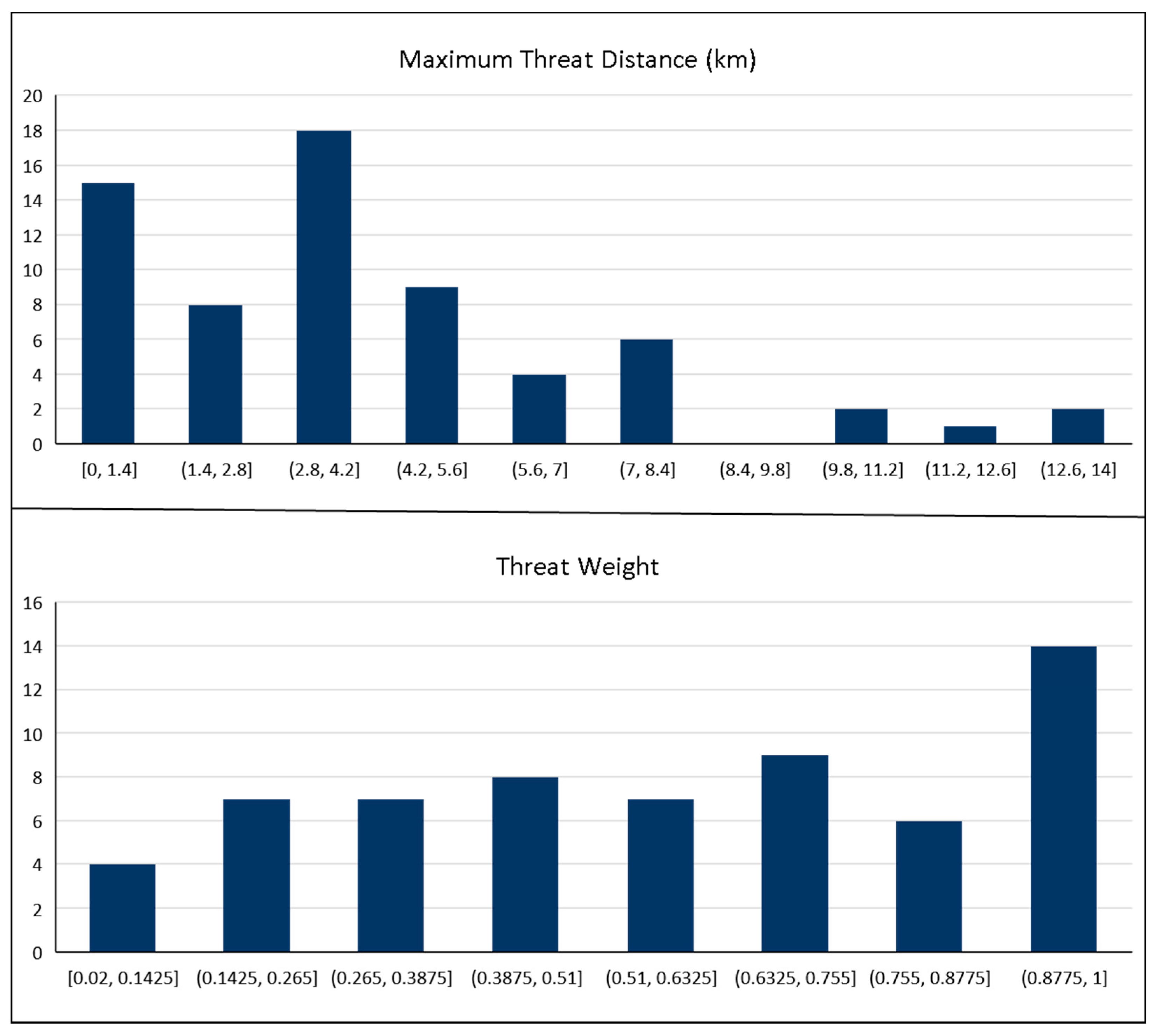
- Analytical results were then summarized in six tables and nine figures. Definitions and descriptions from the literature are shown in Table 1. Most studies did not give a direct definition of “habitat threat”. A definition was derived from what was understood from those studies. Multiple tables were made that list the types of threats, their category based on specificity, and the references that cite each one as well as the sources of available data that were either used in the literature or found by searching the Internet, the variables used to standardize the equations, and a list of threat index estimation equations. Index equations that had directly been found in the literature or had been produced on the basis of the calculation methodology from the literature were compiled. Equations were grouped according to specificity (broad, region-specific, and habitat-specific) and then changed to be more uniform. Similar variables are represented by the same symbol. A bar graph that displays the number of articles per year was created. Figures displaying the meta-analysis results were created by classifying articles used in the analysis by threat type and country of origin. A figure was made to display a tree diagram grouping similar threats and then categorizing them on the basis of how broad or specific the threat is. Another figure displays the country, types of threats, and the number of articles that mention each threat are displayed by using the Layout 5 design of a bar graph in Microsoft Excel 2010. A study distribution map was created by overlaying the number of articles in each country using a photo-editing software called Paint.NET 3.6 developed by dotPDN, LLC at Washington State University in Pullman, Washington, USA. Two histograms were created for the threat characteristics of distance and weight and combined into one figure. The data used to create the figure came from threat-characteristic data found in 11 studies. Finally, a selection tool to aid with choosing the equation that best fits on the basis of obtainable data was made. Equations were first grouped by an identifying variable. The used variables were threat frequency (f), threat severity (α), landscape factor score (L), number of species (S), and threat factor score (F). One equation had nothing in common with the other equations and was placed in its unique group identified by the conversion potential (CP) variable. Equations were then listed in order of complexity.
2.2. Habitat Threat Framework Development
2.3. Habitat Threat Framework Application
3. Results
3.1. Defining Habitat Threat
3.2. Types of Threats
3.3. Available Data
3.4. Characteristics
3.5. Threat Index
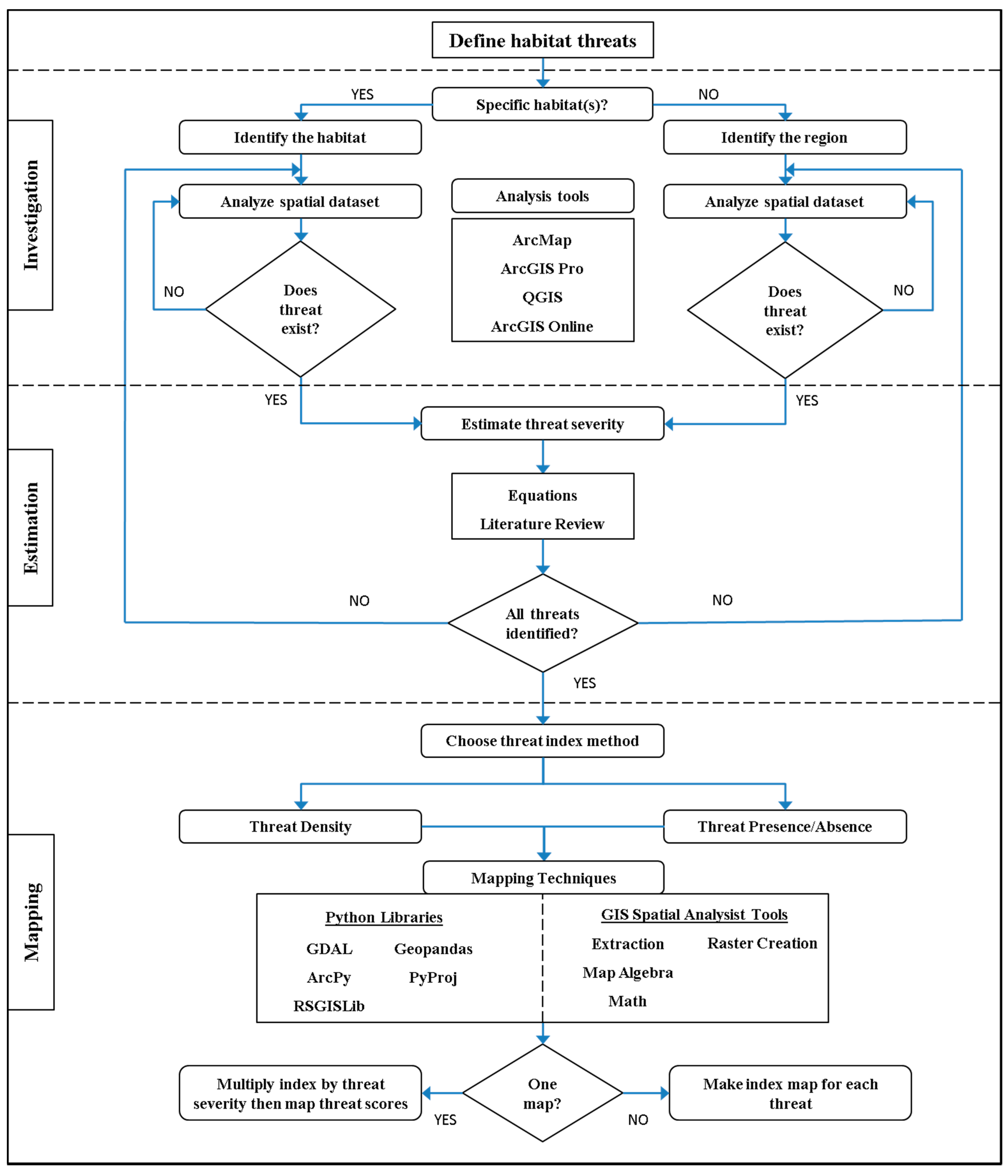
3.6. DIEM Framework
3.7. Application of Framework—Case Study in Choctawhatchee River and Bay Watershed
4. Discussion
4.1. Literature-Review Implications
4.2. Local Threats and Habitats
4.3. Using the DIEM Framework to Produce Threat Maps
4.4. Potential Uses of Threat Maps
4.5. Advantages of the Framework
4.6. Potential Limitations of the Framework and Future Work
5. Conclusions
Supplementary Materials
Author Contributions
Funding
Institutional Review Board Statement
Informed Consent Statement
Data Availability Statement
Conflicts of Interest
References
- Kuemmerlen, M.; Schmalz, B.; Cai, Q.; Haase, P.; Fohrer, N.; Jähnig, S.C. An attack on two fronts: Predicting how changes in land use and climate affect the distribution of stream macroinvertebrates. Freshw. Biol. 2015, 60, 1443–1458. [Google Scholar] [CrossRef]
- Eros, T.; Kuehne, L.; Dolezsai, A.; Sommerwerk, N.; Wolter, C. A systematic review of assessment and conservation management in large floodplain rivers—Actions postponed. Ecol. Indic. 2019, 98, 453–461. [Google Scholar] [CrossRef] [Green Version]
- Sánchez-Bayo, F.; Wyckhuys, K.A. Worldwide decline of the entomofauna: A review of its drivers. Biol. Conserv. 2019, 232, 8–27. [Google Scholar]
- Paukert, C.P.; Pitts, K.L.; Whittier, J.B.; Olden, J.D. Development and assessment of a landscape-scale ecological threat index for the Lower Colorado River Basin. Ecol. Indic. 2011, 11, 304–310. [Google Scholar] [CrossRef]
- Thoms, M.; Sheldon, F. Large rivers as complex adaptive ecosystems. River Res. Appl. 2019, 35, 451–458. [Google Scholar] [CrossRef]
- Strauss, A.; Hurlbutt, B.; O’Brady, C. Preserving Biodiversity. In Colorado College State of the Rockies Report Card; Colorado College: Colorado Springs, CO, USA, 2006; p. 61. [Google Scholar]
- Mehri, A.; Salmanmahiny, A.; Mikaeili Tabrizi, A.R.; Mirkarimi, S.H.; Sadoddin, A. Integration of anthropogenic threats and biodiversity value to identify critical sites for biodiversity conservation. Geocarto Int. 2019, 34, 1202–1217. [Google Scholar] [CrossRef]
- Bell, A.; Matthews, N.; Zhang, W. Opportunities for improved promotion of ecosystem services in agriculture under the Water-Energy-Food Nexus. J. Environ. Stud. Sci. 2016, 6, 183–191. [Google Scholar] [CrossRef]
- Prokopova, M.; Salvati, L.; Egidi, G.; Cudlin, O.; Vcelakova, R.; Plch, R.; Cudlin, P. Envisioning Present and Future Land-Use Change under Varying Ecological Regimes and Their Influence on Landscape Stability. Sustainability 2019, 11, 4654. [Google Scholar] [CrossRef] [Green Version]
- Root, K.V.; Akcakaya, H.R.; Ginzburg, L. A multispecies approach to ecological valuation and conservation. Conserv. Biol. 2003, 17, 196–206. [Google Scholar] [CrossRef]
- Hummel, S.; Calkin, D.E. Costs of landscape silviculture for fire and habitat management. For. Ecol. Manag. 2005, 207, 385–404. [Google Scholar] [CrossRef] [Green Version]
- Peng, F.; Wang, Y.L.; Li, W.F.; Yue, J.; Wu, J.S.; Zhang, Y. Evaluation for sustainable land use in coastal areas: A landscape ecological prospect. Int. J. Sustain. Dev. World Ecol. 2006, 13, 25–36. [Google Scholar] [CrossRef]
- Xu, H.G.; Wu, J.; Liu, Y.; Ding, H.; Zhang, M.; Wu, Y.; Xi, Q.; Wang, L.L. Biodiversity congruence and conservation strategies: A national test. Bioscience 2008, 58, 632–639. [Google Scholar] [CrossRef] [Green Version]
- Baldwin, R.F.; Demaynadier, P.G. Assessing threats to pool-breeding amphibian habitat in an urbanizing landscape. Biol. Conserv. 2009, 142, 1628–1638. [Google Scholar] [CrossRef]
- Payet, K.; Rouget, M.; Esler, K.J.; Reyers, B.; Rebelo, T.; Thompson, M.W.; Vlok, J.H.J. Effect of Land Cover and Ecosystem Mapping on Ecosystem-Risk Assessment in the Little Karoo, South Africa. Conserv. Biol. 2013, 27, 531–541. [Google Scholar] [CrossRef] [PubMed]
- Collen, B.; Whitton, F.; Dyer, E.E.; Baillie, J.E.M.; Cumberlidge, N.; Darwall, W.R.T.; Pollock, C.; Richman, N.I.; Soulsby, A.M.; Bohm, M. Global patterns of freshwater species diversity, threat and endemism. Glob. Ecol. Biogeogr. 2014, 23, 40–51. [Google Scholar] [CrossRef] [Green Version]
- Fore, J.; Sowa, S.; Galat, D.; Annis, G.; Diamond, D.; Rewa, C. Riverine Threat Indices to Assess Watershed Condition and Identify Primary Management Capacity of Agriculture Natural Resource Management Agencies. Environ. Manag. 2014, 53, 567–582. [Google Scholar] [CrossRef]
- Jha, K.K.; McKinley, C.R. Demography and Ecology of Indian Sarus Crane (Grus antigone antigone) in Uttar Pradesh, Northern India. Asian J. Conserv. Biol. 2014, 3, 8–18. [Google Scholar]
- Van Rensselaer, M. A GIS Analysis of Environmental and Anthropogenic Threats to Coastal Archaeological Sites in Southern Monterey County, California. Proc. Soc. Calif. Archaeol. 2014, 28, 373–380. [Google Scholar]
- Mattson, M.K. Modeling Ecological Risks at a Landscape Scale: Threat Assessment in the Upper Tennessee River Basin. 2015. Available online: https://vtechworks.lib.vt.edu/bitstream/handle/10919/78611/Mattson-Hansen_KM_D_2016.pdf?isAllowed=y&sequence=1 (accessed on 7 October 2021).
- Oakleaf, J.R.; Kennedy, C.M.; Baruch-Mordo, S.; West, P.C.; Gerber, J.S.; Jarvis, L.; Kiesecker, J. A World at Risk: Aggregating Development Trends to Forecast Global Habitat Conversion. PLoS ONE 2015, 10, e0138334. [Google Scholar] [CrossRef] [PubMed] [Green Version]
- Tulloch, V.J.D.; Tulloch, A.I.; Visconti, P.; Halpern, B.S.; Watson, J.E.; Evans, M.C.; Auerbach, N.A.; Barnes, M.; Beger, M.; Chadès, I.; et al. Why do we map threats? Linking threat mapping with actions to make better conservation decisions. Front. Ecol. Environ. 2015, 13, 91–99. [Google Scholar] [CrossRef] [Green Version]
- Khobe, D.; Akosim, C.; Kwaga, B.T. Susceptibility to Threats and Threat Severity of Adamawa Rangelands, Nigeria. J. Adv. Agric. 2016, 5, 698–705. [Google Scholar]
- Verkamp, H.J. Stream benthic algal relationships with multimetric indices of sensitivity, exposure, and vulnerability to watershed land use change, with an emphasis on unconventional natural gas development. Biol. Sci. 2016. Available online: https://scholarworks.uark.edu/cgi/viewcontent.cgi?article=1011&context=biscuht (accessed on 7 October 2021).
- Armendariz, G.; Quiroz-Martinez, B.; Alvarez, F. Risk assessment for the Mexican freshwater crayfish: The roles of diversity, endemism and conservation status. Aquat. Conserv.-Mar. Freshw. Ecosyst. 2017, 27, 78–89. [Google Scholar] [CrossRef] [Green Version]
- Turak, E.; Harrison, I.; Dudgeon, D.; Abell, R.; Bush, A.; Darwall, W.; Finlayson, C.M.; Ferrier, S.; Freyhof, J.; Hermoso, V.; et al. Essential Biodiversity Variables for measuring change in global freshwater biodiversity. Biol. Conserv. 2017, 213, 272–279. [Google Scholar] [CrossRef]
- Kim, Y.; Kong, I.; Park, H.; Kim, H.J.; Kim, I.J.; Um, M.J.; Green, P.A.; Vorosmarty, C.J. Assessment of regional threats to human water security adopting the global framework: A case study in South Korea. Sci. Total Environ. 2018, 637, 1413–1422. [Google Scholar] [CrossRef] [PubMed]
- Deffense, N. Deriving a habitat quality index to inform reef conservation in the Great Barrier Reef. In Faculté des Bioingénieurs; Université Catholique de Louvain: Louvain-la-Neuve, Belgium, 2019; p. 78. [Google Scholar]
- Mashizi, A.K.; Sharafatmadrid, M. Assessing Impact of Anthropogenic Disturbances on Forage Production in Arid and Semiarid Rangelands. J. Rangel. Sci. 2019, 9, 234–245. [Google Scholar]
- Nelson, E.; Ennaanay, D.; Wolny, S.; Olwero, N.; Vigerstol, K.; Pennington, D.; Mendoza, G.; Aukema, J.; Foster, J.; Forrest, J.; et al. InVEST 3.8.0. User’s Guide. Sharp, R., Chaplin-Kramer, R., Wood, S., Guerry, A., Tallis, H., Ricketts, T., Eds.; 2020. Available online: https://invest-userguide.readthedocs.io/_/downloads/en/3.8.3/pdf/ (accessed on 7 October 2021).
- Groves, C. Drafting a Conservation Blueprint: A Practitioner’s Guide to Planning for Biodiversity; Island Press: Washington, DC, USA, 2003; p. 458. [Google Scholar]
- Wilson, T.S.; Sleeter, B.M.; Sleeter, R.R.; Soulard, C.E. Land-Use Threats and Protected Areas: A Scenario-Based, Landscape Level Approach. Land 2014, 3, 362–389. [Google Scholar] [CrossRef] [Green Version]
- Blair, P.; Buytaert, W. Socio-hydrological modelling: A review asking“ why, what and how?”. Hydrol. Earth Syst. Sci. 2016, 20, 443–478. [Google Scholar] [CrossRef] [Green Version]
- Patrício, J.; Elliott, M.; Mazik, K.; Papadopoulou, K.-N.; Smith, C.J. DPSIR—Two Decades of Trying to Develop a Unifying Framework for Marine Environmental Management? Front. Mar. Sci. 2016, 3, 177. [Google Scholar] [CrossRef]
- Livingston, R.; Epler, J.; Jordan, F.; Karsteter, W.; Koenig, C.; Prasad, A.; Ray, G. Ecology of the Choctawhatchee River System; Springer: New York, NY, USA, 1991; pp. 247–274. [Google Scholar]
- CPYRWMA. Choctawhatchee River. 2017. Available online: https://cpyrwma.alabama.gov/about-the-watersheds-choctawhatchee-river/ (accessed on 28 March 2021).
- Hall, L.S.; Krausman, P.R.; Morrison, M.L. The habitat concept and a plea for standard terminology. Wildl. Soc. Bull. 1997, 25, 173–182. [Google Scholar]
- Turlure, C.; Van Dyck, H.; Schtickzelle, N.; Baguette, M. Resource-based habitat definition, niche overlap and conservation of two sympatric glacial relict butterflies. Oikos 2009, 118, 950–960. [Google Scholar] [CrossRef]
- Amorim, J.; Hendrix, M.; Andler, S.; Gustavsson, P. Gamified Training for Cyber Defence: Methods and Automated Tools for Situation and Threat Assessment in Nato Modelling & Simulation Group (NMSG) Multi-Workshop, MSG-111. 2013. Available online: File:///C:/Users/Admin/Downloads/2013-P055-010-54-SYDNEY2-paper18_NATO-Cyber.pdf (accessed on 7 October 2021).
- Barnett, T.P.; Pierce, D.W.; Schnur, R. Detection of Anthropogenic Climate Change in the World’s Oceans. Science 2001, 292, 270–274. [Google Scholar] [CrossRef] [Green Version]
- Cook, J.; Oreskes, N.; Doran, P.; Anderegg, W.R.L.; Verheggen, B.; Maibach, E.W.; Carlton, S.; Lewandowsky, S.; Skuce, A.G.; Green, S.A. Consensus on consensus: A synthesis of consensus estimates on human-caused global warming. Environ. Res. Lett. 2016, 11, 048002. [Google Scholar] [CrossRef]
- Hook, M.; Tang, X. Depletion of fossil fuels and anthropogenic climate change—A review. Energy Policy 2012, 52, 797–809. [Google Scholar] [CrossRef] [Green Version]
- Travis, J.M.J. Climate change and habitat destruction: A deadly anthropogenic cocktail. R. Soc. 2003, 270. [Google Scholar] [CrossRef] [Green Version]
- Calizza, E.; Costantini, M.L.; Careddu, G.; Rossi, L. Effect of habitat degradation on competition, carrying capacity, and species assemblage stability. Ecol. Evol. 2017, 7, 5784–5796. [Google Scholar] [CrossRef]
- Fargione, J.E.; Cooper, T.R.; Flaspohler, D.J.; Hill, J.; Lehman, C.; McCoy, T.; McLeod, S.; Nelson, E.J.; Oberhauser, K.S.; Tilman, D. Bioenergy and Wildlife: Threats and Opportunities for Grassland Conservation. Bioscience 2009, 59, 767–777. [Google Scholar] [CrossRef] [Green Version]
- Wilcove, D.S.; Rothstein, D.; Dubow, J.; Phillips, A.; Losos, E. Quantifying threats to imperiled species in the United States. Bioscience 1998, 48, 607–615. [Google Scholar] [CrossRef] [Green Version]
- Entrekin, S.A.; Maloney, K.O.; Kapo, K.E.; Walters, A.W.; Evans-White, M.A.; Klemow, K.M. Stream Vulnerability to Widespread and Emergent Stressors: A Focus on Unconventional Oil and Gas. PLoS ONE 2015, 10, e0137416. [Google Scholar] [CrossRef] [PubMed]
- Gibson, D.M.; Quinn, J.E. Application of Anthromes to Frame Scenario Planning for Landscape-Scale Conservation Decision Making. Land 2017, 6, 33. [Google Scholar] [CrossRef] [Green Version]
- Li, F.X.; Wang, L.Y.; Chen, Z.J.; Clarke, K.C.; Li, M.C.; Jiang, P.H. Extending the SLEUTH model to integrate habitat quality into urban growth simulation. J. Environ. Manag. 2018, 217, 486–498. [Google Scholar] [CrossRef] [Green Version]
- Polasky, S.; Nelson, E.; Lonsdorf, E.; Fackler, P.; Starfield, A. Conserving species in a working landscape: Land use with biological and economic objectives. Ecol. Appl. 2005, 15, 1387–1401. [Google Scholar] [CrossRef] [Green Version]
- Radeloff, V.C.; Nelson, E.; Plantinga, A.G.; Lewis, D.J.; Helmers, D.; Lawler, J.J.; Withey, J.C.; Beaudry, F.; Martinuzzi, S.; Butsic, V.; et al. Economic-based projections of future land use in the conterminous United States under alternative policy scenarios. Ecol. Appl. 2012, 22, 1036–1049. [Google Scholar] [CrossRef] [Green Version]
- Sleeter, B.M.; Sohl, T.L.; Loveland, T.R.; Auch, R.F.; Acevedo, W.; Drummond, M.A.; Sayler, K.L.; Stehman, S.V. Land-cover change in the conterminous United States from 1973 to 2000. Glob. Environ. Chang.-Hum. Policy Dimens. 2013, 23, 733–748. [Google Scholar] [CrossRef] [Green Version]
- Sowa, S.; Annis, G.; Morey, M.; Diamond, D. A gap analysis and comprehensive conservation strategy for riverine ecosystems of Missouri. Ecol. Monogr. 2007, 77, 301–334. [Google Scholar] [CrossRef]
- Wang, L.; Brenden, T.; Seelbach, P.; Cooper, A.; Allan, D.; Clark, R.; Wiley, M. Landscape Based Identification of Human Disturbance Gradients and Reference Conditions for Michigan Streams. Environ. Monit. Assess. 2008, 141, 1–17. [Google Scholar] [CrossRef] [PubMed]
- Chengxin, W.; Changbo, Q.; Hongdi, L.; Yan, S. Exploration of Ecological Space Identification and Ecological Impact Assessment in Planning Environmental Impact Assessment —A Case Study of Changchun New District Development Planning. Chin. J. Environ. Manag. 2017, 9, 88–94. [Google Scholar] [CrossRef]
- Wang, R.; Jiang, Y.; Su, P.; Wang, J.A. Global Spatial Distributions of and Trends in Rice Exposure to High Temperature. Sustainability 2019, 11, 6271. [Google Scholar] [CrossRef] [Green Version]
- Yunzhe, D.; Jiangfeng, L.; Jianxin, Y. SpatiotemporalresponsesofhabitatqualitytourbansprawlintheChangsha metropolitanarea. Prog. Geogr. 2018, 37, 11. [Google Scholar] [CrossRef]
- Terrado, M.; Sabater, S.; Chaplin-Kramer, B.; Mandle, L.; Ziv, G.; Acuna, V. Model development for the assessment of terrestrial and aquatic habitat quality in conservation planning. Sci. Total Environ. 2016, 540, 63–70. [Google Scholar] [CrossRef] [Green Version]
- Zhang, H.B.; Wu, F.E.; Zhang, Y.N.; Hans, S.; Liu, Y.Q. Spatial and temporal changes of habitat quality in Jiangsu Yancheng wetland national nature reserve—Rare birds of China. Appl. Ecol. Environ. Res. 2019, 17, 4807–4821. [Google Scholar] [CrossRef]
- Galarraga, K.S.R. Evaluación del Servicio Ecosistémico de Calidad del Habitat Presente en la Cuenca Alta y Media del Río Coca Mediante el Uso del Paquete Computacional Invest 3.3.1, in Facultad De Ingeniería Civil y Ambiental. 2019. Available online: file:///C:/Users/Admin/Downloads/CD-9446.pdf (accessed on 5 October 2021).
- Meyer, J.M. Modeling the Impact of Gold Mining on Ecosystem Services in Ghana´s Southern Water Basins in Geospatial Technologies. 2019. Available online: https://run.unl.pt/bitstream/10362/63813/1/TGEO0214.pdf (accessed on 5 October 2021).
- Xu, L.T.; Chen, S.S.; Xu, Y.; Li, G.Y.; Su, W.Z. Impacts of Land-Use Change on Habitat Quality during 1985–2015 in the Taihu Lake Basin. Sustainability 2019, 11, 3513. [Google Scholar] [CrossRef] [Green Version]
- Lina, Z.; Jun, W. Evaluation on effect of land consolidation on habitat quality based on InVEST model. Trans. Chin. Soc. Agric. Eng. 2017, 33, 250–255. [Google Scholar] [CrossRef]
- Ryu, J.-E.; Choi, Y.-y.; Jeon, S.-W.; Sung, H.-C. Evaluation of Habitat Function of National Park Based on Biodiversity and Habitat Value. Korean Environ. Res. Technol. 2018, 21, 39–60. [Google Scholar] [CrossRef]
- Lemos, A.B. Evaluating Ecosystem Services Trade-Offs Due to Land Use Changes: Transition to an Irrigated Agriculture Landscape in Departamento de Biologia Animal. 2017. Available online: https://repositorio.ul.pt/bitstream/10451/27672/1/ulfc120781_tm_Ana_Lemos.pdf (accessed on 5 October 2021).
- Vogelmann, J.E.; Howard, S.M.; Yang, L.; Larson, C.R.; Wylie, B.K.; Van Driel, J.N. Completion of the 1990s National Land Cover Data set for the conterminous United States from Landsat Thematic Mapper data and ancillary data sources. Photogramm. Eng. Remote Sens. 2001, 67, 650–662. [Google Scholar]
- Yang, L.; Jin, S.; Danielson, P.; Homer, C.; Gass, L.; Bender, S.M.; Case, A.; Costello, C.; Dewitz, J.; Fry, J.; et al. A new generation of the United States National Land Cover Database: Requirements, research priorities, design, and implementation strategies. ISPRS J. Photogramm. Remote Sens. 2018, 146, 108–123. [Google Scholar] [CrossRef]
- Jin, S.; Homer, C.; Yang, L.; Danielson, P.; Dewitz, J.; Li, C.; Zhu, Z.; Xian, G.; Howard, D. Overall Methodology Design for the United States National Land Cover Database 2016 Products. Remote Sens. 2019, 11, 2971. [Google Scholar] [CrossRef] [Green Version]
- Fry, J.A.; Coan, M.; Homer, C.G.; Meyer, D.K.; Wickham, J.D. Completion of the National Land Cover Database (NLCD) 1992–2001 Land Cover Change Retrofit Product, in Open-File Report. 2009. Available online: https://pubs.usgs.gov/of/2008/1379/pdf/ofr2008-1379.pdf (accessed on 7 October 2021).
- Huang, C.; Goward, S.N.; Masek, J.G.; Thomas, N.; Zhu, Z.; Vogelmann, J.E. An automated approach for reconstructing recent forest disturbance history using dense Landsat time series stacks. Remote Sens. Environ. 2010, 114, 183–198. [Google Scholar] [CrossRef]
- Roy, D.P.; Ju, J.; Kline, K.L.; Scaramuzza, P.L.; Kovalskyy, V.; Hansen, M.; Loveland, T.; Vermote, E.; Zhang, C. Web-enabled Landsat Data (WELD): Landsat ETM+ composited mosaics of the conterminous United States. Remote Sens. Environ. 2010, 114, 35–49. [Google Scholar] [CrossRef]
- Johnson, D.M. Using the Landsat archive to map crop cover history across the United States. Remote Sens. Environ. 2019, 232. [Google Scholar] [CrossRef]
- Eidenshink, J.C.; Schwind, B.; Brewer, K.; Zhu, Z.; Quayle, B.; Howard, S. A Project for Monitoring Trends in Burn Severity. Fire Ecol. 2007, 3, 3–21. [Google Scholar] [CrossRef]
- WFIGS, W.F.I.G.S. WFIGS-2021 Wildland Fire Locations to Date. 2021. Available online: https://data-nifc.opendata.arcgis.com/datasets/nifc::wfigs-2021-wildland-fire-locations-to-date/about (accessed on 1 July 2021).
- DHS, D.o.H.S. HIFLD Open Data. 2020. Available online: https://hifld-geoplatform.opendata.arcgis.com/ (accessed on 1 July 2021).
- USEIA. Layer Information for Interactive State Maps. 2020. Available online: https://www.eia.gov/maps/layer_info-m.php (accessed on 13 June 2020).
- Prospect- and Mine-Related Features from U.S. Geological Survey 7.5- and 15-Minute Topo-graphic Quadrangle Maps of the United States. Available online: https://www.sciencebase.gov/catalog/item/5a1492c3e4b09fc93dcfd574 (accessed on 5 October 2021).
- USGS. NAS—Nonindigenous Aquatic Species. 2020. Available online: https://nas.er.usgs.gov/viewer/omap.aspx (accessed on 13 June 2020).
- Bargeron, C.; LaForest, J.; Bush, B.; Carroll, R.; Daniel, J.; Dasari, S.; Wallace, R. Distribution Maps. 2021. Available online: https://www.eddmaps.org/distribution/ (accessed on 1 July 2021).
- Ruefenacht, B.; Finco, M.V.; Nelson, M.D.; Czaplewski, R.; Helmer, E.H.; Blackard, J.A.; Holden, G.R.; Lister, A.J.; Salajanu, D.; Weyermann, D.; et al. Conterminous U.S. and Alaska Forest Type Mapping Using Forest Inventory and Analysis Data. Photogramm. Eng. Remote Sens. 2008, 74, 1379–1388. [Google Scholar] [CrossRef]
- National Geospatial Program, U. National Hydrography. 2020. Available online: https://www.usgs.gov/core-science-systems/ngp/national-hydrography (accessed on 12 July 2020).
- WorldPop. Population Density. 2021. Available online: https://www.worldpop.org/project/categories?id=18 (accessed on 1 July 2021).
- Czech, B.; Krausman, P.R.; Devers, P.K. Economic Associations among Causes of Species Endangerment in the United States. Bioscience 2000, 50, 593–601. [Google Scholar] [CrossRef] [Green Version]
- Nie, C.; Yang, J.; Huang, C.H. Assessing the Habitat Quality of Aquatic Environments in Urban Beijing. Procedia Environ. Sci. 2016, 36, 162–168. [Google Scholar] [CrossRef] [Green Version]
- Shen, Y.; Cao, H.; Tang, M.; Deng, H. The Human Threat to River Ecosystems at the Watershed Scale: An Ecological Security Assessment of the Songhua River Basin, Northeast China. Water 2017, 9, 219. [Google Scholar] [CrossRef] [Green Version]


| Definition/Description | Examples | Context/Objective | References |
|---|---|---|---|
| Economic development activities that cause a risk of species extinction | Urban development | Ecological conservation | [10] |
| Events causing disturbances to habitat structure | Wildfires | Fire and habitat management | [11] |
| Pressure imposed on landscapes through human activity | Urbanization, agriculture | Sustainable land-use evaluation | [12] |
| Things that hinder biodiversity | Threats in order: habitat destruction, invasive species, climate change, pollution, overexploitation, habitat fragmentation, and disease | Preserving biodiversity | [6] |
| Activities that pose a risk to species richness and endemism | Agricultural activity, forestry, animal husbandry, fishery, invasive species | Species conservation | [13] |
| Stressors that cause habitat degradation | Urbanization | Pool-breeding amphibian habitat assessment | [14] |
| Anthropogenic disturbances | Agriculture, urbanization, road and railroad density, pollution sites, canals, and dams | Freshwater ecosystem assessment | [4] |
| Practices that transform the ecosystem | Urbanization, cultivation (i.e., forestry plantation), grazing, mining, introduction of invasive species | Ecosystem risk assessment | [15] |
| Stresses on the ecosystem | Agriculture, industry, domestic activity, water extraction, introduction of exotic species, dams and reservoirs, and pollution | Freshwater species conservation | [16] |
| Human activities | Agriculture, urban, point-source pollution, infrastructure, and nonagricultural threats | Conservation of lotic systems | [17] |
| Anthropogenic activities that alter the natural state of the habitat | Pollution, agricultural expansion, removal of soil for various purposes, removal of vegetation (extraction of consumable products), expansion of vegetation (spread of weeds), land encroachment, fishing, siltation | Indian Sarus Crane habitat conservation | [18] |
| Negative human and environmental impacts | Sea-level rise | Coastal archaeological site preservation | [19] |
| Human-related impact. | Mining and agriculture | Freshwater conservation | [20] |
| Habitat conversion due to development | Urbanization, agriculture, fossil fuel energy, renewable energy, mining | Global habitat | [21] |
| Human activities that drive species loss and ecosystem change | Open-cut mining, grazing, oil-palm production, and coastal urban development | Conservation planning | [22] |
| Factors that put biodiversity at risk | Natural threats: erosion, floods, droughts, disease, pests; human-induced threats: population pressure, overexploitation of biological resources, uncontrolled introduction of exotic species, poaching, fire, war; political threats | Rangeland resources/biodiversity | [23] |
| Things that put the health and condition of ecosystems at risk | Unconventional natural-gas development | Watershed | [24] |
| Things that pose a risk to species richness and endemism | Human activities | Mexican freshwater crayfish conservation | [25] |
| Things that change species diversity, distribution, and conservation status. Activities that pose a risk to species richness and endemism | None listed | Freshwater biodiversity | [26] |
| Human activities that impact water resources | Increasing population, land cover changes in watersheds, urban expansion, and intensive use of freshwater resources | Water-resource management and security | [27] |
| Something that poses a risk to a habitat | Thermal stress, cyclone damage, land-based pollutants, and predation. Main threat is climate change | Risk to coral-reef habitats | [28] |
| Human activities | Agriculture, urbanization, river regulations (channelization, dams, flood control by levees) | Large floodplain river conservation | [2] |
| Anthropogenic factors that impact ecosystem services | Urbanization, construction, agriculture, and invasive species | Forage production | [29] |
| A human-modified land-use/cover type that causes habitat fragmentation, edge, and degradation in neighboring habitats | Agriculture and urbanization | Habitat quality | [30] |
| Level | Threat (Number) | References |
|---|---|---|
| I | Natural (9) | [6,9,11,19,23,27,28,45,46] |
| II | Climate change (5) | [6,9,19,27,28] |
| Disease (3) | [6,23,46] | |
| Predation (1) | [28] | |
| Pests (1) | [23] | |
| Wildfire (2) | [11,45] | |
| III | Extreme weather (1) | [28] |
| Erosion (1) | [23] | |
| Floods (1) | [23] | |
| Droughts (1) | [23] | |
| Sea-level rise (1) | [19] |
| Level | Threat (Number) | References |
|---|---|---|
| I | Anthropogenic (43) | [2,4,6,9,10,12,13,14,15,16,17,18,20,21,22,23,24,25,26,27,28,29,37,46,47,48,49,50,51,52,53,54,55,56,57,58,59,60,61,62,63,64,65] |
| II | Resource use (6) | [2,4,6,13,16,27] |
| Pollution (4) | [4,16,18,28] | |
| Development/industry (4) | [16,56,61,64] | |
| Fire (1) | [23] | |
| War (1) | [23] | |
| LULC change (7) | [9,20,27,49,50,51,52] | |
| Invasive species (9) | [6,9,13,15,29,46,51,58,59] | |
| III | Habitat destruction (4) | [6,18,46,47] |
| Habitat fragmentation (1) | [6] | |
| Overexploitation (4) | [6,9,23,46] | |
| Water use (4) | [16,27,58,63] | |
| Poaching (1) | [23] | |
| Fishery (2) | [13,59] | |
| Land-based pollutants (1) | [28] | |
| Thermal stress (1) | [28] | |
| Agriculture (18) | [2,4,12,13,16,17,18,21,29,53,55,56,57,58,60,61,62,63] | |
| Urbanization (20) | [2,4,10,12,14,15,17,21,22,27,29,48,49,53,55,57,58,61,62,65] | |
| Forestry (1) | [13] | |
| Infrastructure (1) | [17] | |
| Population pressure (3) | [23,27,53] | |
| Fossil-fuel energy (3) | [21,24,47] | |
| Mining (8) | [15,21,22,52,58,61,62,63] | |
| Bioenergy (1) | [45] | |
| IV | River regulations (1) | [2] |
| Canals (2) | [4,58] | |
| Dams (4) | [4,16,58,60] | |
| Reservoirs (1) | [16] |
| Dataset | Date (s) | Description | Scale/Resolution | References |
|---|---|---|---|---|
| National Land Cover Dataset (NLCD) | 1992, 2001, 2006, 2011, 2016, 2019 | Land-cover data | 30 m | [66,67,68] |
| NLCD Land Cover Change Index | 2001, 2004, 2006, 2008, 2011, 2013, 2016, 2019 | Land cover change data | 30 m | [67] |
| NLCD Retro Product | 1992, 2001 | Retrofitted 1992–2001 land-cover change data | 30 m | [69] |
| LANDFIRE’s Vegetation Change Tracker (VCT) | 1984–2016 | Annual forest disturbance | 30 m | [70] |
| Web-enabled Landsat Data (WELD) | 2006–2014 | Forest decline data | 30 m | [71] |
| Cropland Data Layer (CDL) | 1997–2019 | Crop cover history | 30 to 56 m | [72] |
| Monitoring Trends in Burn Severity (MTBS) | 1984–2019 | Burn severity and wildfire data | 30 m | [73] |
| Wildland Fire Interagency Geospatial Services (WFIGS) | 1970–2020 | Point location for reported fires in the US | N/A | [74] |
| Homeland Infrastructure Foundation Layer Data (HIFLD) | 2019–2020 | National foundation-level geospatial data within the open public domain such as mining, energy, and natural hazards | N/A | [75] |
| U.S. Energy Information Administration (USEIA) maps | 2019–2020 | Map layers for various energy-related things such as biofuel and power plants | ≥50 m | [76] |
| Prospect- and mine-related features map | 2019 | Mining-related features digitized from historical USGS topographic maps | 1:24,000 scale to 1:62,500 scale | [77] |
| Nonindigenous Aquatic Species (NAS) data | Real-time | Map of invasive-species sightings | 1:100,000 scale | [78] |
| Early Detection and Distribution Mapping System (EDDMapS) | Real-time | Web-based maps of invasive-species distribution | N/A | [79] |
| National Forest Type Dataset | 2004 | 141 forest types across the US | 250 m | [80] |
| National Hydrography Dataset (NHD) | 2018 | Map of surface water networks, including canals and dams | 10 m | [81] |
| WorldPop population data | 2000–2020 | Population counts and density datasets | 30 arc-seconds ~1 km | [82] |
| Symbol | Description |
|---|---|
| HTI | Habitat threat index |
| HTIc | Habitat threat index at target grid cell |
| HTIj | Habitat threat index for land use j |
| HTIse | Habitat threat index for stream segment s in ecoregion e |
| C | Number of grid cells |
| Cc | Number of grid cells with score less than target cell |
| CPcP | Conversion potential—likelihood of land conversion projected for each grid cell |
| DTPA | Distance to protected area |
| F | Threat factor index/ranking/score |
| H | Habitat value or suitability—ability of a habitat to support life |
| L | Landscape factor index/ranking/score |
| LULCc | Land-use/land-cover change |
| N | Number of grid cells |
| Nc | Number of grid cells for land use type |
| Nl | Number of land uses |
| PL | Protection level |
| Ps | Projected scenario |
| S | Number of species |
| X | Probability of extinction |
| e | Ecoregion |
| f | Threat frequency—how often a threat occurs (grid cells) |
| j | Land use type |
| k | Threat metric |
| n | Total number of threat factors or landscape factors |
| ns | Number of stream segments |
| s | Stream segments |
| y | Year |
| α | Threat impact or severity |
| β | Coefficient for linear regression |
| γji | Contribution of land use j on the viability of species i |
| σ | Standard deviation |
| Specificity | Region/Habitat | Equation | References |
|---|---|---|---|
| Broad | Various regions | [10] | |
| Global | [21] | ||
| Region-specific | Mountain range | [6] | |
| Lower Colorado River Basin | [4] | ||
| Watershed | [27] | ||
| Habitat-specific | Wetlands | [14] | |
| Prairie, desert, steppe | [17] | ||
| Coastal | [19] | ||
| Coast, lowlands, cascades | [32] | ||
| Rangelands | [23] | ||
| Aquatic habitats | [84] | ||
| Freshwater | [25] | ||
| River ecosystems | [85] | ||
| Great Barrier Reef | [28] |
Publisher’s Note: MDPI stays neutral with regard to jurisdictional claims in published maps and institutional affiliations. |
© 2021 by the authors. Licensee MDPI, Basel, Switzerland. This article is an open access article distributed under the terms and conditions of the Creative Commons Attribution (CC BY) license (https://creativecommons.org/licenses/by/4.0/).
Share and Cite
Muhammed, K.; Anandhi, A.; Chen, G.; Poole, K. Define–Investigate–Estimate–Map (DIEM) Framework for Modeling Habitat Threats. Sustainability 2021, 13, 11259. https://doi.org/10.3390/su132011259
Muhammed K, Anandhi A, Chen G, Poole K. Define–Investigate–Estimate–Map (DIEM) Framework for Modeling Habitat Threats. Sustainability. 2021; 13(20):11259. https://doi.org/10.3390/su132011259
Chicago/Turabian StyleMuhammed, Khaleel, Aavudai Anandhi, Gang Chen, and Kevin Poole. 2021. "Define–Investigate–Estimate–Map (DIEM) Framework for Modeling Habitat Threats" Sustainability 13, no. 20: 11259. https://doi.org/10.3390/su132011259