Dynamic and Static Analysis of Carbon Emission Efficiency in China’s Transportation Sector

Abstract

As the main undesirable output of the transportation sector, carbon dioxide (CO₂) emission is the key point to achieving carbon balance in the whole sector. In this paper, the bounded adjustment measure (BAM) data envelopment analysis method is used to measure the total factor production (TFP) efficiency of transportation system and the source of its inefficiency. Based on this, we use the global Malmquist index combined with the BAM to analyze the key factors of environmental productivity change from 2004 to 2019 in terms of dynamic changes in technology level, production scale and management efficiency. The results show that the main reasons for the low efficiency of carbon emission production in China’s transportation sector are unreasonable energy utilization, excess labor resources and excessive CO₂ emission caused by low technology level. Further analysis shows that China’s overall environmental production efficiency has begun to show a slow rising trend. Improvement of management level is the biggest driving force for the growth of total factor productivity of China’s transportation sector, while the improvement of scale and technology should be strengthened for the improvement of overall production efficiency. There are spatial differences in the production efficiency of China’s transportation sector. In the future, different provinces should focus on improving the production efficiency of transport industry.

1. Introduction

Human activities are expected to have caused about 1.0 °C of global warming, compared to the pre-industrial levels, and its possible value is between 0.8 °C to 1.2 °C. According to the Intergovernmental Panel on Climate Change (IPCC), it is expected that this value could reach 1.5 °C between 2030 and 2052 if the increasing rate of global warming remains the same [1]. Global carbon dioxide emissions have increased dramatically in the last few decades and are expected to increase in the future [2]. As a major emitter of carbon dioxide, China is under pressure both at home and abroad to cut emissions. In September 2020, China’s carbon dioxide emissions should peak before 2030 and become carbon-neutral by 2060, according to the Central Economic Work Conference. In its 13th Five-Year Plan (2016–2020), the Chinese government announced another target for carbon emissions to peak around 2030. In this context, China’s total transport energy consumption will reach 1.03 billion tons of oil equivalent in 2023. Of the total, oil consumption will reach 831 million tons, 1.71 times of China’s consumption of 488 million tons in 2013, and accounting for 2.1 percent of China’s oil production in 2013 (3.95 billion tons). According to the International Energy Agency (IEA), the transportation sector is the world’s third largest source of carbon dioxide emissions, behind manufacturing and electricity production [3]. It is predicted that in 2030, it will reach more than four times that in 2000. How to effectively control the carbon emission of transportation industry has become one of the important aspects in China’s energy-saving reduction. China’s systematic energy conservation and emission reduction is still facing various problems, and there is increasing pressure on this energy conservation and emission reduction. China’s transportation industry is energy inefficient and carbon emission intensive, so it is very important to analyze the productivity of transportation system, find the source of production inefficiency and then improve productivity to meet these serious challenges [4,5]. In this context, calculating and analyzing the level of inefficiency and energy saving, production efficiency and its dynamic changes in the transportation industry can help scholars and decision makers clarify gains and losses, output feedback mechanisms for subsequent policy adjustment and improvement and determine the appropriate direction and focus of future work. In this paper, the dynamic and static changes of total factor production efficiency of carbon emissions in China’s provincial transportation sector are calculated and are further decomposed. In particular, we focus on the dynamic evolution of CO₂ emissions at provincial levels. In addition, we combine the Theil index to analyze the spatial differences.

The rest of this article is as follows: Section 2 reviews the related literature. Section 3 gives the methods and models. Section 4 provides an overview of the data set. Section 5 is the empirical results and analysis. Section 6 gives the conclusion and suggestions.

2. Literature Review

Data envelopment analysis (DEA) is a non-parametric efficiency evaluation method [6]. Energy efficiency research can be divided into two categories depending on the type of indicators used. One is the study of the single-factor index based on energy intensity. The other is the study based on total factor index, which often uses DEA and stochastic frontier analysis (SFA) to measure total factor productivity. At present, single-factor and all-factor indicators have been widely used in the comparison of eco-environmental assessment, the exploration of eco-environmental influencing factors and the prediction of eco-environmental assessment between regions and industries [7]. However, in the single-factor research framework, the relationship between the input and output of energy consumption is obtained, and the potential substitution effect between other factors such as labor intensity is ignored. In addition, the single-factor research framework differs greatly from the actual production process, and the estimates based on this analysis method cannot measure the actual production efficiency. Hu and Wang [8] developed a total factor analysis method in accordance with the objective law in which multiple factors work together on economic output. Song et al. [9] and Zhou et al. [6] extended the research framework of total factor productivity to analyze such problems. This total factor framework is widely used to measure regional, national and sectoral energy efficiency [10,11,12].

China’s transportation sector is a major driver of increased energy consumption and carbon emissions in the coming decades and is the sector most likely to fail to reach peak carbon emissions by 2030. It is very important to study the change of transportation system productivity and its influencing factors. This can provide scientific guidance for China’s transportation sector to formulate timely strategies to achieve the goal of “dual carbon”. In fact, many studies have tried to do just that. Zhang et al. [13] estimated the carbon emission efficiency of the transportation industry in 30 provinces of China during 2008–2017. Zhao et al. [14] used the epsilon-measure DEA model to estimate the CO₂ emission efficiency of China’s provincial transportation sector. Xie et al. [15] calculated the energy efficiency of the provincial transportation sector in China from 2007 to 2016 and gave the energy saving and emission reduction potential of the provinces. Zha et al. [16] used the provincial panel data over 2005–2016 to perform regression analysis. Existing relevant research often uses an input-oriented analysis method or single output-oriented model but ignores the analysis of the unified production efficiency of input and output, and it is difficult to evaluate the objective comprehensive level of the development of the transportation sector. Lei et al. [17] applied multidirectional efficiency analysis (MEA) to measure the regional energy and production efficiency of China’s transportation sector. Chang et al. [18] adopted the slackness-based measure (SBM) to analyze the environmental efficiency. Cui and Li [19] proposed three-level virtual frontier data enveloping analysis (three-level virtual frontier data enveloping analysis) to evaluate transportation energy efficiency, but they do not take into account unexpected outputs such as carbon dioxide. Wu et al. [20] regarded the transportation system as a parallel system composed of passenger and freight sub-systems and extended the parallel DEA method to evaluate the efficiency. Stefaniecet et al. [21] introduced a systematic approach based on the triple bottom line to evaluate inland transport, taking into account sustainability.

The economic development of China’s transportation sector is very different in different regions. For example, there is a big difference in production technology between eastern and western regions. Many studies do not take this situation into full consideration, which may lead to the estimation bias in the evaluation of production efficiency [19,22,23]. To fill this gap in the literature, Feng and Wang [24] tried to use the global meta-frontier DEA method to eliminate the impact of such regional heterogeneity on energy efficiency. Shi et al. [25] used the Moran ‘I index and the Getis-Ord Gi index to analyze the temporal dynamic changes and spatial autocorrelation of carbon emission production efficiency in the transportation industry. Li et al. [26] analyzed the efficiency differences among different economic regions in China. It is concluded that technological progress and technological efficiency are the key to improve the efficiency of carbon emission and energy emission in China. In addition, Wang et al. [27] used super-efficiency DEA and the Theil index to analyze the differences and changes of regional energy efficiency in China’s transportation sector. Xia et al. [28] used a meta-frontier DEA-based decomposition approach to measure the spatial carbon intensity inequality.

We can see that DEA has become a mainstream method to measure production efficiency and energy efficiency. The above scholars focus on traditional models, such as traditional radial models such as CCR and BCC, as well as non-radial models such as SBM and RAM. The traditional radial model is input-oriented and assumes that all inputs should be scaled to achieve maximum efficiency. This assumption is contrary to the actual production operation. It is difficult for various elements to expand or decrease in the same proportion. Compared with the CCR and BCC models, the BAM model has the characteristics of non-radial and undirected, that is, the input (output) variables may change proportionally. Li and Hu [29] calculated the total factor energy efficiency of 30 regions in China by using the SBM model of undesired output. Zhang and Choi [30] used three DEA models to evaluate China’s regional economy from 2001 to 2010, avoiding the limitations brought on by the radial model with decreasing factor proportion. Li et al. [31] constructed the Super-SBM model under the condition of output accident, which solved the problem with multiple decision-making units simultaneously, reaching the optimal production efficiency. Huang et al. [32] proposed a model combining cutting-edge production technology, poor output and super-efficiency SBM to further explore the dynamic changes of regional eco-efficiency in China. Wang et al. [33] used the global DEA model to study China’s energy efficiency from static and dynamic perspectives. Compared with relax-based measures (i.e., relax-based measures, SBM), the BAM model significantly avoids the setting of subjective parameters and ensures the objectivity of efficiency scores. Emrouznejad and Yang [34] used the global MLP index based on RAM to evaluate the CO₂ emission efficiency of China’s light industry. Miao et al. [35] proposed a range adjustment metric (RAM) based on additive structure to measure changes in management level, technical efficiency and pure efficiency. Note that we distinguish among energy and non-energy inputs in the analysis. Different from RAM, the BAM model has a strong ability to discriminate low efficiency scores, that is, the BAM model of different DMUs has a large difference in low efficiency. In addition, BAM works with any return to scale, whereas traditional RAM may not have a solution with constant return to scale.

Although the BAM-DEA model can objectively reflect energy efficiency and environmental production efficiency due to its unique advantages, as a data envelopment analysis method, it can only measure the static inefficiency rather than the dynamic change in time. To overcome these shortcomings, this paper combines the BAM-DEA method with the Malmquist productivity index to measure dynamic change.

Table 1. Comparison of research methods on carbon emission in China’s transportation sector.

Authors	Method	Malmquist Used	Inefficiencies	Heterogeneity
Chang et al. [18]	SBM-DEA	No	No	No
Zhou et al. [22]	DDF-DEA	No	Yes	No
Feng and Wang [24]	DEA, meta-frontier	Yes	No	Yes
Xie et al. [15]	SFA	No	No	No
Lei et al. [17]	Ratio-based parallel DEA	No	No	No
Chen et al. [36]	BAM-DEA	No	Yes	No
Zhang et al. [13]	Metaglobal frontier DEA model	Yes	No	No
Zha et al. [16]	Super-efficiency DEA	Yes	No	No
Stefaniec et al. [21]	Triple bottom line-based network DEA	No	Yes	No
Zhao et al. [14]	EBM-DEA	No	No	Yes
This study	BAM-DEA	Yes	Yes	Yes

Note: DEA—Data envelopment analysis; SBM—slack-based measure; BAM—bounded-adjusted measure; EBM—epsilon-based measure; SFA—stochastic frontier analysis; DDF—directional distance function.

gives the comparison of research methods on carbon emission in China’s transportation sector.

3. Materials and Methods

3.1. Environmental Production Technology

The expression of production technology is mainly characterized by input and output. In the production activities related to carbon emission, they mainly include effective output and undesirable output. Undesired outputs are mainly related to energy inputs, so we divide the input into energy inputs and non-energy inputs. It is technically unfeasible for an enterprise to try to reduce the undesirable output alone, and it needs to pay a certain economic cost to reduce the undesirable output. The production technology is described by the following set of production possibilities:

$$T_E=\left\{\right(x, y, b) \in R_{+}^{N+M+J}: x\mathit{can}\mathit{produce} (y, b\left)\right\}.$$

(1)

This is the case for a producer who employs a vector of inputs $X=\left(x_1,\dots ,x_N\right)\in R_{+}^N$ to produce a vector of desirable $Y=\left(y_1,\dots ,y_N\right)\in R_{+}^M$ and undesirable outputs $B=\left(b_1,\dots ,b_N\right)\in R_{+}^J$. The original data set S is defined as $S={{\displaystyle \cup }}_{t=1}^T(X_t,Y_t,B_t)$, and the yearly specific data set is defined as $S_t=\left(X_t,Y_t,B_t\right),t=1,2,\dots T$.

We further describe the production of desired and undesired outputs following two commonly used assumptions [37,38,39]:

Assumption 1.

Null-jointness assumption

$$\mathit{If} \left(x,y,b\right)\in T_E \mathit{and} b=0, \mathit{then}y=0.$$

Assumption 2.

Weakly disposable assumption

$$\mathit{If} \left(x,y,b\right)\in T_E \mathit{and} 0\le \theta \le 1, \mathit{then} \left(x,{\theta }_y,{\theta }_b\right)\in T_E.$$

Assumption 1 implies that the undesirable output is a by-product of the production of the desired product, and that if the undesirable product were to be eliminated completely, the desired output would also be eliminated. Assumption 2 shows that the reduction in unexpected output comes at the cost of a simultaneous proportional reduction in desired output, and this hypothesis can reasonably reflect the cost of the need to eliminate unexpected output. With these two assumptions as the premise, production technology T_i can realistically simulate the joint production process of a sector i based on production activities. For each sector, suppose K regions (k = 1, …, K) are under evaluation. In empirical studies, in order to better represent the production technology, a non-parametric linear method is usually given to model the technology. The environmental production technology is defined as

$$T=\{\left(x,y,b\right):{\displaystyle \sum }_k{\lambda }_k{x}_k\le x,{\displaystyle \sum }_k{\lambda }_k{y}_k\ge y,{\displaystyle \sum }_k{\lambda }_k{b}_k\ge b,{\lambda }_k\ge 0,k=1,\dots ,K\}.$$

(2)

where λ denotes intensity variable.

3.2. Measure of Production Efficiency

BAM-DEA was proposed by Cooper et al. [40] and extended by Chen et al. [36], in which a new method was formulated to separate unexpected outputs from the BAM model. Inefficiency is indicated by ${\rho }_o$ for DMU under evaluation $\left(x_o,y_o,b_o\right)$ (o = 1, …, K) and is related to the maximization of slack variables $s_n^x;s_m^y;s_j^b$. The BAM-DEA model is as follows:

$${\rho }_o=\mathit{max}\frac{[{\sum }_{n=1}^N{\displaystyle \frac{s_n^x}{L_n^x}}+{\sum }_{m=1}^M{\displaystyle \frac{s_m^y}{U_m^y}}+{\sum }_{j=1}^J{\displaystyle \frac{s_j^b}{L_j^b}}]}{N+M+J}$$

(3)

$$\begin{gathered} s.t. \\ {x}_{n{k}^{\prime }}={\displaystyle \sum }_{k=1}^K{\lambda }_K{x}_{nk}+s_n^x,n=1,2,\dots ,N \end{gathered}$$

(4)

$$y_{m{k}^{\prime }}={\displaystyle \sum }_{k=1}^K{\lambda }_K{y}_{mk}-s_m^y,m=1,2,\dots ,M.$$

(5)

$$b_{j{k}^{\prime }}={\sum }_{k=1}^K{\lambda }_K{b}_{jk}+s_j^b,j=1,2,\dots ,J$$

(6)

$${\sum }_{k=1}^K{\lambda }_K{x}_{nk}\ge \mathit{min}{x}_{nk},n=1,2,\dots ,N$$

(7)

$${\displaystyle \sum }_{k=1}^K{\lambda }_K{y}_{mk}\le \mathit{max}{y}_{mk},m=1,2,\dots ,M$$

(8)

$${\sum }_{k=1}^K{\lambda }_K{b}_{jk}\ge \mathit{min}{b}_{jk},j=1,2,\dots ,J$$

(9)

$${\displaystyle \sum }_{k=1}^K{\lambda }_K=1$$

(10)

$${\lambda }_K,s_n^x,s_m^y,s_j^b\ge 0$$

(11)

where ${\rho }_o;s_n^x;s_m^y;s_j^b$ are respectively the efficiency score, excess input, expected output deficit and excess of unexpected output. Potential emission reduction per decision-making unit is estimated by slack variable $s_j^b$, as it emits more carbon than the optimal decision-making unit. ($L_n^x,U_m^y,L_j^b$) represents the difference between the maximum input value, ideal output and non-ideal output and itself, specifically as follows:

$$L_n^x=x_{nk}-\mathit{min}(x_{nk})$$

(12)

$$U_m^y=\mathit{max}(y_{mk})-y_{mk}$$

(13)

$$L_j^b=b_{jk}-\mathit{min}(b_{jk})$$

(14)

We can find that when the ith input meets $x_{nk}=\mathit{min}(x_{nk})$, the production technology frontier cannot be reached by increasing or decreasing the input (i.e., $\frac{s_n^x}{L_n^x}=0$). Similarly, the element of output satisfies this property. While $\mathit{max}(y_{mk})=y_{mk},b_{jk}=\mathit{min}(b_{jk})$, we obtain $\frac{s_m^y}{U_m^y}=0,\frac{s_j^b}{L_j^b}=0$.

According to Cooper et al. [41], we adopt the same decomposition idea. Since the method in this paper and SBM belong to the same additive model, the decomposition method is also applicable to the BAM model. We can obtain the inefficiency score of each variable as follows:

Inefficiency in the inputs: $I{E}_x=\frac{{\sum }_{n=1}^N\frac{s_n^x}{L_n^x}}{N+M+J}$.

Inefficiency in the good outputs: $I{E}_y=\frac{{\sum }_{m=1}^M\frac{s_m^y}{U_m^y}}{N+M+J}$.

Inefficiency in the bad outputs: $I{E}_b=\frac{{\sum }_{j=1}^J\frac{s_j^b}{L_j^b}}{N+M+J}$.

Therefore, the expression of productivity and production inefficiency of provincial transportation system is $E=1-{\rho }_o,IE=I{E}_x+I{E}_y+I{E}_b={\rho }_o$.

3.3. The Global Malmquist Index Based on BAM

The Malmquist index is a widely used method for measuring productivity and decomposing efficiency/productivity changes. In order to make the calculation results of the index cyclic and avoid the infeasibility of linear programming, a global Malmquist index used to decompose the changes in productivity and efficiency is adopted, motivated by [42]. Here, let $P^t$ and $P^G$ respectively represent the same period and global production frontier technology. Let T be the study period. Concretely, $P^t$ and $P^G$ can respectively be written as follows:

$$P^t=\{(y^t,b^t)|x^t can produce (y^t,b^t)\}$$

(15)

$$P^G=P^1\cup P^2\cup ,\dots ,\cup P^T$$

(16)

The expression of Malmquist exponential function from t to t + 1 is

$$M^{t,t+1}={[\frac{1-{\rho }^{t+1}(x^{t+1},y^{t+1},b^{t+1}|CRS)}{1-{\rho }^{t+1}(x^t,y^t,b^t|CRS)}\times \frac{1-{\rho }^t(x^{t+1},y^{t+1},b^{t+1}|CRS)}{1-{\rho }^t(x^t,y^t,b^t|CRS)}]}^{\frac{1}{2}}$$

(17)

where $1-{\rho }^{t+1}(x^{t+1},y^{t+1},b^{t+1}|CRS)$ and $1-{\rho }^{t+1}(x^t,y^t,b^t|CRS)$ are the total factor production efficiency in periods t + 1 and t, respectively, referring to $P^t$ under CRS; $1-{\rho }^t(x^{t+1},y^{t+1},b^{t+1}|CRS)$ and $1-{\rho }^t(x^t,y^t,b^t|CRS)$ are the total factor production efficiency in periods t + 1 and t, respectively, referring to $P^t$ under CRS.

By introducing the global concept, the GM index to estimate the change of productivity efficiency during t and t + 1 can be written as

$$G{M}^{t,t+1}=\frac{1-{\rho }^G(x^{t+1},y^{t+1},b^{t+1}|CRS)}{1-{\rho }^G(x^t,y^t,b^t|CRS)}$$

(18)

where $1-{\rho }^G(x^{t+1},y^{t+1},b^{t+1}|CRS)$ and $1-{\rho }^G(x^t,y^t,b^t|CRS)$ are the total factor production efficiency in periods t + 1 and t, respectively, referring to global leading production technology ${\rho }^G$ under CRS. The factorization of GM index is expressed as follows:

$$G{M}^{t,t+1}=GTC{H}_{t,t+1}\times GPC{H}_{t,t+1}\times GSC{H}_{t,t+1}$$

(19)

$$GTC{H}_{t,t+1}=\frac{1-{\rho }^G(x^{t+1},y^{t+1},b^{t+1}|CRS)}{1-{\rho }^{t+1}(x^{t+1},y^{t+1},b^{t+1}|CRS)}\backslash \frac{1-{\rho }^G(x^t,y^t,b^t|CRS)}{1-{\rho }^t(x^t,y^t,b^t|CRS)}$$

(20)

$$GPC{H}_{t,t+1}=\frac{1-{\rho }^{t+1}(x^{t+1},y^{t+1},b^{t+1}|VRS)}{1-{\rho }^t(x^t,y^t,b^t|VRS)}$$

(21)

$$GSC{H}_{t,t+1}=\frac{1-{\rho }^{t+1}(x^{t+1},y^{t+1},b^{t+1}|CRS)}{1-{\rho }^t(x^t,y^t,b^t|VRS)}\backslash \frac{1-{\rho }^t(x^t,y^t,b^t|CRS)}{1-{\rho }^t(x^t,y^t,b^t|VRS)}$$

(22)

where $GTC{H}_{t,t+1}$, $GPC{H}_{t,t+1}$ and $GSC{H}_{t,t+1}$ denote technological changes, pure efficiency changes and scale efficiency changes, respectively. Technical change (GTCH), pure efficiency change (GPCH) and scale efficiency change (GSCH) are decomposed by the GM index. Zhou et al. [6] showed that a GTCH value greater than 1 indicates technological progress compared with the previous period. A GPCH value greater than 1 indicates an increase in net efficiency compared to the previous period. A GSCH value greater than 1 indicates that the scale efficiency is improved compared with the previous period, while a value less than 1 indicates that the scale efficiency is reduced.

3.4. The Theil Index Decomposition Analysis

The Theil index can be used to evaluate the regional difference of an index. The higher the value, the greater the regional difference. Tian et al. [43] applied The Theil index to analyze the imbalance of regional carbon emission intensity in China. In this paper, the Theil index is used to measure the overall difference of GM index of carbon emissions from the transportation industry in 30 provincial administrative regions, which is decomposed into the difference between three economic zones and the difference within the region. Among them, the three major economic zones include the eastern, central and western regions. The Theil index and its decomposition can be calculated as

$$I_p=\frac{1}{n_p}{\sum }_{i=1}^N\frac{G_{pi}}{{\overline{G}}_p}\mathit{ln}\frac{G_{pi}}{{\overline{G}}_p}$$

(23)

$$I_w={\sum }_{p=1}^M(\frac{n_p}{n}\frac{G_p}{\overline{G}})I_p$$

(24)

$$I_B={\sum }_{p=1}^M\frac{n_p}{n}(\frac{G_p}{\overline{G}})\mathit{ln}\frac{G_i}{{\overline{G}}_i}$$

(25)

$$I=I_B+I_w=\frac{1}{n}{\sum }_{i=1}^N\frac{G_i}{\overline{G}}\mathit{ln}\frac{G_i}{\overline{G}}$$

(26)

where $I$ represents the overall Theil index of the 30 provincial administrative regions, based on the GM index within the research scope, which can be broken down into the difference between the three major economic regions $I_B$, and the difference between the provinces in each major economic region $I_w$. $G_i$ is the GM index value of the $i$th province, $\overline{G}$ is the average value of the GM index of each province, $G_{pi}$ is the GM index of each province in the p region and ${\overline{G}}_p$ is its corresponding average value. $I_p$ is the Theil index of the GM index of provinces in the p region.

4. Data Source and Description

The data set used in this paper includes 16-year input and output data of the transport industry in 30 provinces of the Chinese mainland (2004–2019). The raw data contain three inputs: labor, capital stock and fuel consumption, as well as desirable output (gross sector value added) and undesirable output (CO₂).

Table 2. Summary statistics of inputs and outputs.

Variable	Unit	Observations	Mean	Min	Max	Std.
Labor	1000 persons	480	716.27	20.11	641.73	110.52
Capital	Billion CNY	480	499.25	3.55	3003.75	521.83
Fuel consumption	1000 TCE	480	1001.96	31.56	3814.82	666.56
Value-added	Billion CNY	480	82.29	3.05	365.8	69.94
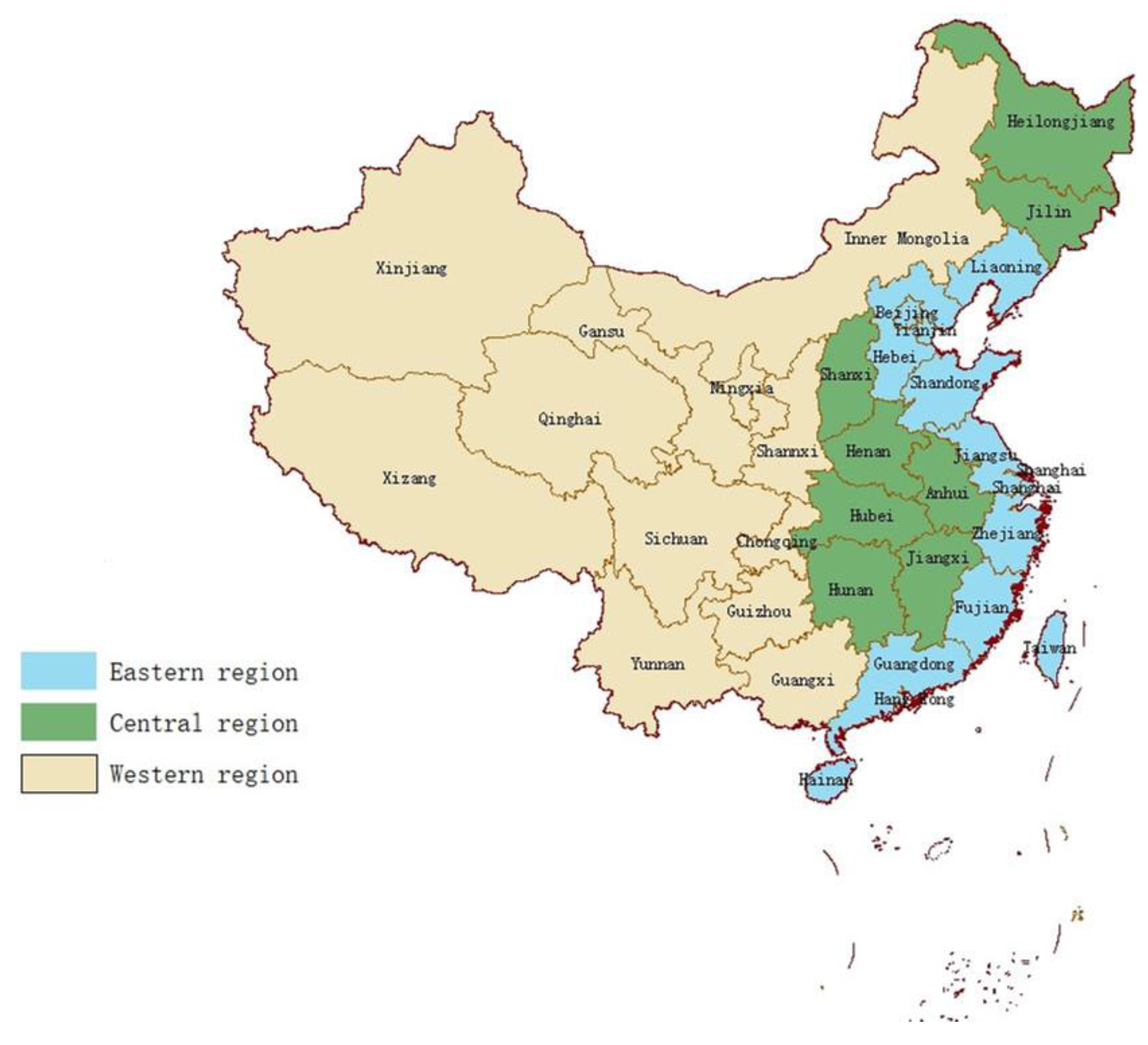
CO2	10,000 tons	480	2325.64	77.93	8562.12	1564.51

provides a summary statistic of inputs and outputs. In this study, regional groups are determined according to geographical distance and economic level, and the research objects are divided into three regional groups: east, central and west (as shown in Figure 1).

(1) Labor: The total labor force in each province is the labor input. The data used are from the China Statistical Yearbook (2005–2020).

(2) Fuel consumption: Fuel consumption is expressed in tons of standard coal equivalent (TCE). Conversion factors are acquired from the China Energy Statistical Yearbook. The energy consumption data are gathered from all provincial statistical yearbooks.

(3) Capital stock: Capital input is calculated using the perpetual inventory method. According to the provincial fixed asset investment price index, the nominal fixed asset investment of the whole society is adjusted to the constant price in 2008 to obtain this value. We use the perpetual inventory method to estimate the capital amount, which can be expressed as $K_t=\left(1-{\delta }_t\right)K_{t-1}+M_t$, where $K_t$ and $K_{t-1}$ mean the DMU’s capital stock in years t and t − 1, respectively. $M_t$ denotes the investment in the fixed asset in year t, and ${\delta }_t$ denotes the depreciation rate, which is 10.96% [44]. We use fixed asset investment in 2008 as the equity for the beginning year. Data are collected from the China Statistical Yearbook (2005–2020).

(4) Desirable output: We use each province’s value-added as a measure of expected output and adjust it to constant 2004 prices based on each province’s value-added deflator, which are required from the China Statistical Yearbook (2009–2020).

(5) Undesirable output: According to the carbon emission accounting method provided by IPCC, this paper adopts the fuel-based carbon calculation model and conversion factor to calculate carbon emission. Carbon dioxide emissions are calculated by the following formula:

$$C{O}_{2}emissions={\displaystyle \sum }_l{A}_l\times CC{F}_l\times H{E}_l\times CO{F}_l\times \frac{44}{12}$$

(27)

The carbon dioxide emission is equal to the product of the amount burned of all carbonized fuels (A), the carbon content factor (CCF), the thermal equivalent (HE), the carbon oxidation factor of carbonized fuels (COF) and the number (44/12).

5. Empirical Results and Discussion

5.1. Analysis on the Inefficiencies

Based on the improved BAM-DEA model, we calculate the total factor productivity of the transportation sector in 30 provincial regions of China in the whole sample period. This paper lists the inefficiency (IE) of the input variable (X), the transport added value (Y) as the desirable output variable and the CO₂ emission (b) as the undesirable output for the period 2004–2019. Results are obtained using Python 3.7.2 (Continuum Analytics, Austin, TX, USA). Table 2 shows the result of efficiency scores assuming CRS.

As can be seen from

Table 3. The productivity of transportation sectors in China during 2004–2019.

Region and Province		Productivity
		2004	2005		2006	2007	2008	2009	2010	2011
Eastern region	Beijing	0.5556	0.5511		0.4880	0.4425	0.3641	0.3488	0.3930	0.3875
	Tianjin	1.0000	1.0000		0.7359	0.7157	0.7205	0.6745	0.7263	0.7319
	Hebei	1.0000	1.0000		1.0000	1.0000	1.0000	1.0000	1.0000	1.0000
	Liaoning	0.5316	0.4786		0.4677	0.4693	0.4264	0.4075	0.3831	0.3855
	Shanghai	0.5846	0.6070		0.5789	0.5310	0.4890	0.4120	0.4721	0.4312
	Jiangsu	0.4930	0.5964		0.6494	0.6982	0.6854	0.6294	0.6065	0.9024
	Zhejiang	0.5485	0.5643		0.6032	0.6407	0.6124	0.5740	0.6269	0.5943
	Fujian	1.0000	1.0000		1.0000	1.0000	1.0000	0.7290	0.6827	0.5930
	Shandong	0.5563	0.7359		1.0000	1.0000	1.0000	1.0000	0.4847	0.5639
	Guangdong	0.5652	0.6000		0.6224	0.6370	0.4288	0.3766	0.3703	0.3843
	Hainan	0.4276	0.4689		0.2477	0.2451	0.2293	0.1980	0.1949	0.1928
Central region	Shanxi	0.5812	0.5222		0.5636	0.6296	0.5744	0.4250	0.4052	0.3935
	Jilin	0.5524	0.4707		0.4945	0.4639	0.4078	0.3797	0.3756	0.3858
	Heilongjiang	0.4165	0.4043		0.3778	0.3780	0.3331	0.2805	0.2844	0.2607
	Anhui	1.0000	1.0000		1.0000	1.0000	1.0000	0.8802	1.0000	1.0000
	Jiangxi	0.4784	0.5404		0.5718	0.5860	0.5211	0.4769	0.4741	0.4679
	Henan	0.6035	0.6473		0.7307	0.8015	0.6832	0.6749	0.6281	0.6207
	Hubei	0.4176	0.4442		0.4641	0.4633	0.4410	0.4594	0.5121	0.4992
	Hunan	0.5158	0.5544		0.5761	0.5893	0.5881	0.5485	0.5515	0.5258
Western region	Inner Mongolia	0.6357	0.4790		0.4908	0.4842	0.4730	0.4511	0.4339	0.4242
	Guangxi	0.4020	0.3805		0.3597	0.3492	0.3468	0.3351	0.3661	0.3757
	Chongqing	0.4075	0.4509		0.4991	0.4461	0.4512	0.4506	0.4570	0.4512
	Sichuan	0.4613	0.4797		0.4986	0.4828	0.4107	0.3647	0.3326	0.3155
	Guizhou	0.2567	0.2739		0.2760	0.2911	0.2983	0.2775	0.2814	0.2761
	Yunnan	0.4183	0.2907		0.3514	0.3680	0.2882	0.2801	0.2809	0.2753
	Shaanxi	0.3775	0.4052		0.4488	0.4357	0.4137	0.3809	0.3867	0.3861
	Gansu	0.3160	0.3502		0.4075	0.3898	0.4109	0.3739	0.4817	0.5021
	Qinghai	0.6047	1.0000		1.0000	1.0000	0.6618	0.5938	0.5919	0.5900
	Ningxia	0.7221	0.4696		0.6484	0.6586	0.8763	0.6068	0.5997	0.5980
	Xinjiang	0.3206	0.2727		0.2609	0.2680	0.2491	0.2359	0.2335	0.2165
Average		0.5583	0.5679		0.5804	0.5822	0.5462	0.4942	0.4872	0.4910
Region and Province		Productivity
		2012	2013	2014	2015	2016	2017	2018	2019	Average
Eastern region	Beijing	0.3636	0.3802	0.3944	0.3784	0.4177	0.4241	0.4400	0.4569	0.4241
	Tianjin	0.6418	0.6654	0.6091	0.5003	0.5908	0.5306	0.5139	0.6200	0.6860
	Hebei	1.0000	1.0000	1.0000	1.0000	1.0000	1.0000	1.0000	1.0000	1.0000
	Liaoning	0.3941	0.3964	0.3948	0.4135	0.4877	0.4687	0.4961	0.5319	0.4458
	Shanghai	0.4220	0.4460	0.4990	0.5281	0.6102	0.6431	1.0000	1.0000	0.5784
	Jiangsu	1.0000	0.9000	0.8806	0.6647	0.7485	0.6970	0.7107	0.7303	0.7245
	Zhejiang	0.5710	0.5908	0.5904	0.5955	0.6628	0.6221	0.6004	0.7542	0.6095
	Fujian	0.5783	0.5460	0.5360	0.5305	0.5833	0.5454	0.5298	0.6254	0.7175
	Shandong	0.5917	0.6102	0.6632	0.5915	0.6876	0.8283	0.7859	0.6745	0.7358
	Guangdong	0.4033	0.3877	0.3978	0.5862	0.6229	0.4143	0.4136	0.6869	0.4936
	Hainan	0.1944	0.1944	0.1952	0.1987	0.4554	0.1995	0.1965	0.3983	0.2648
Central region	Shanxi	0.4082	0.3667	0.3671	0.3807	0.4041	0.4214	0.4873	0.5448	0.4672
	Jilin	0.3972	0.3925	0.3793	0.3677	0.3664	0.3286	0.3225	0.3167	0.4001
	Heilongjiang	0.2674	0.2622	0.2818	0.2832	0.2860	0.2709	0.2635	0.2529	0.3065
	Anhui	1.0000	1.0000	1.0000	1.0000	1.0000	1.0000	1.0000	1.0000	0.9925
	Jiangxi	0.6006	0.5547	0.5498	0.5102	0.5771	0.5834	0.6758	0.7704	0.5587
	Henan	0.7032	1.0000	0.8795	1.0000	1.0000	1.0000	1.0000	1.0000	0.8108
	Hubei	0.5159	0.5503	0.5781	0.5734	0.5848	0.5716	0.5887	0.6600	0.5202
	Hunan	0.5676	0.5573	0.5600	0.5520	0.5868	0.5617	0.5581	0.5864	0.5612
Western region	Inner Mongolia	0.4361	0.4365	0.4643	0.4578	0.5174	0.4943	0.4886	0.5603	0.4830
	Guangxi	0.3706	0.4021	0.3860	0.3784	0.4168	0.3913	0.3805	0.4256	0.3792
	Chongqing	0.4128	0.3877	0.3960	0.3750	0.4045	0.3912	0.3912	0.4593	0.4270
	Sichuan	0.3141	0.3296	0.3649	0.3548	0.4061	0.3777	0.4077	0.4575	0.3974
	Guizhou	0.2666	0.2851	0.2961	0.3239	0.3394	0.3103	0.3170	0.3711	0.2963
	Yunnan	0.3102	0.3342	0.3520	0.3483	0.3952	0.4015	0.4301	0.4878	0.3508
	Shaanxi	0.4150	0.4020	0.4329	0.4186	0.4756	0.4484	0.4412	0.5218	0.4244
	Gansu	0.4438	0.4729	0.2993	0.2987	0.2849	0.2813	0.2382	0.2614	0.3633
	Qinghai	0.7910	0.5907	0.5911	0.5928	0.3993	0.3933	0.3905	0.3908	0.6364
	Ningxia	0.3995	0.5986	0.5979	0.5992	0.6624	0.7975	0.7932	0.5938	0.6388
	Xinjiang	0.2497	0.2606	0.2966	0.3099	0.3130	0.3047	0.3614	0.3882	0.2838
Average		0.5010	0.5100	0.5078	0.5037	0.5429	0.5234	0.5408	0.5842	0.5326

, the average annual production efficiency of 30 provincial-level regions in China during 2004–2019 is 0.53.

At the regional level, the efficiency of the three regions is significantly different. The eastern region efficiency score is 0.58, the central region is 0.55 and the western region is 0.40, which shows that the changes of total factor productivity between regions are not balanced and there are certain spatial differences. Hebei, Henan, Anhui and Shandong provinces scored more than 0.7 points in productivity during the study period. On the contrary, Qinghai, Hainan, Gansu and Xinjiang provinces scored relatively lower on productivity. In general, there is a large spatial imbalance in the total factor productivity of carbon emissions in China’s transportation industry, which is mainly affected by the economic development status and policies of various provinces.

From the sources of inefficiency in

Table 4. Inefficiencies for China’s province-level regions.

Region and Province	Sources of Inefficiency
		IE	IEx	IEy	IEb
Eastern region	Beijing	0.5759	0.4049	0	0.1710
	Tianjin	0.3140	0.2054	0	0.1086
	Hebei	0	0	0	0
	Liaoning	0.5542	0.3893	0	0.1648
	Shanghai	0.4216	0.2799	0	0.1417
	Jiangsu	0.2755	0.0938	0.1222	0.0595
	Zhejiang	0.3905	0.2814	0	0.1092
	Fujian	0.2825	0.2033	0	0.0793
	Shandong	0.2642	0.0928	0.1082	0.0632
	Guangdong	0.5064	0.2698	0.1125	0.1241
	Hainan	0.7352	0.5585	0.0023	0.1744
Central region	Shanxi	0.5328	0.3720	0	0.1608
	Jilin	0.5999	0.4218	0	0.1781
	Heilongjiang	0.6935	0.5024	0	0.1912
	Anhui	0.0075	0.0034	0	0.0040
	Jiangxi	0.4413	0.3184	0	0.1230
	Henan	0.1892	0.1519	0	0.0374
	Hubei	0.4798	0.3303	0	0.1494
	Hunan	0.4388	0.3069	0	0.1319
Western region	Inner Mongolia	0.5170	0.3561	0	0.1609
	Guangxi	0.6208	0.4441	0	0.1768
	Chongqing	0.5730	0.4031	0	0.1699
	Sichuan	0.6026	0.4364	0	0.1662
	Guizhou	0.7037	0.5066	0	0.1971
	Yunnan	0.6492	0.4723	0	0.1769
	Shaanxi	0.5756	0.4141	0	0.1615
	Gansu	0.6367	0.4408	0	0.1959
	Qinghai	0.3636	0.2905	0.0053	0.0678
	Ningxia	0.3612	0.2097	0.0014	0.1500
	Xinjiang	0.7162	0.5193	0	0.1969
Average		0.4674	0.3226	0.0117	0.1331

, overall, the average productivity inefficiency in mainland China is as high as 0.47. This means that the transportation sector in mainland China is less productive. The overall inefficiency of industry added value is close to zero (0.01). This shows that the whole department still pays more attention to economic benefits, ignoring the improvement of production technology. This also agrees with China’s output performance. In fact, its average GDP growth between 2004 and 2019 was between 6 and 10 per cent. If the transportation sector still blindly pursues economic development, regardless of the improvement of the overall factor production efficiency, the potential of economic growth will soon be restricted. Input efficiency (0.32) and CO₂ emission efficiency (0.13) were relatively high, accounting for 69.6% and 28.2% of the overall efficiency, respectively. This means that China’s transportation sector has great potential to reduce investment, labor and CO₂ emissions. Excessive emissions of environmental pollutants such as CO₂ remain the biggest cause of low productivity in the transport sector in mainland China.

At the regional level, input-induced inefficiency in western China is 0.41, which is significantly higher than that in eastern China (0.25) and central China (0.30). This is mainly because China has been developed in processing and manufacturing for many years and has a large population. During the year we studied, China had a very high proportion of labor-intensive industries. Especially in the central and western regions, as the technology and equipment are obviously inferior to the central and eastern regions, a large number of enterprises mainly rely on manual labor to create profits. Therefore, the Chinese mainland has a large number of redundant labor force phenomenon. China is a major emitter of carbon dioxide, with relatively high carbon dioxide emissions per unit of GDP and relatively low carbon dioxide emissions per capita. China’s carbon efficiency is at a low level.

5.2. Analysis of Efficiency Changes

In this section, we analyze the key factors that lead to changes in productivity over time by looking at changes in the GM index and its decomposition index. The GM index of transportation carbon emissions in 30 provincial administrative regions in China from 2004 to 2019 was calculated, and the results are shown in

Table 5. Provincial transportation sectors’ GM index during 2004–2019.

Provinces	2004–2005	2005–2006	2006–2007	2007–2008	2008–2009	2009–2010	2010–2011	2011–2012
Beijing	0.8737	0.8958	0.9643	0.9272	0.9756	1.1285	1.0204	0.8390
Tianjin	0.6637	1.0595	1.0299	1.0600	0.9133	1.0613	1.0724	0.8529
Hebei	0.7356	1.1045	1.1489	1.0713	0.9907	0.9826	1.0272	0.9812
Shanxi	0.7995	1.0223	1.1214	0.9908	0.8611	0.9773	1.0095	0.9936
Inner Mongolia	0.7026	1.0475	1.0338	1.0458	0.9369	0.9528	1.0280	0.9842
Liaoning	0.7697	1.0009	1.0322	1.0097	0.9900	0.9692	1.0355	0.9809
Jilin	0.7858	1.0318	0.9984	0.9670	1.0222	1.0028	1.0922	0.9869
Heilongjiang	0.8562	0.9398	1.0629	1.0608	0.9301	1.0737	0.8978	1.0154
Shanghai	0.9882	0.9870	0.9277	0.9337	0.8559	1.1396	0.9689	0.9248
Jiangsu	1.1122	1.0806	1.0890	1.0984	0.9626	1.0622	1.0510	0.9822
Zhejiang	0.9984	1.0492	1.0390	1.0019	0.9534	1.0980	1.0014	0.9250
Anhui	0.9324	1.0207	0.9948	1.0563	0.8872	0.9616	0.9869	0.8985
Fujian	0.7732	1.0616	1.2183	0.7989	0.8963	0.9558	0.9386	0.9397
Jiangxi	1.0607	1.0556	1.0458	1.0170	0.9797	0.9751	1.0417	1.1342
Shandong	0.9024	1.1476	1.0193	1.4275	0.6988	0.9465	1.0562	0.9568
Henan	0.9664	1.1190	1.0892	0.9525	1.0236	0.9216	1.0190	1.0560
Hubei	0.9469	1.0427	1.0181	1.0204	1.0695	1.1472	1.0055	0.9875
Hunan	0.9210	1.0287	1.0654	1.1369	0.9759	0.9835	0.9987	1.0234
Guangdong	0.9405	1.0324	1.0559	1.0564	0.8970	0.9973	1.0082	0.9868
Guangxi	0.8736	0.9518	1.0449	1.1249	1.0201	1.0478	1.0680	0.9581
Hainan	0.5136	1.0256	1.0437	0.9854	0.9901	1.0819	1.1045	1.0866
Chongqing	1.0438	1.1173	0.9902	1.0783	0.9784	1.0002	1.0342	0.8885
Sichuan	0.9344	1.0297	1.0168	0.9735	0.9063	0.9040	1.0135	0.9728
Guizhou	1.1706	1.0909	1.1520	1.0279	0.9618	0.9917	1.0815	0.9809
Yunnan	0.7078	1.2040	1.0966	0.8635	0.9959	0.9918	1.0534	1.0656
Shaanxi	0.9788	1.1114	1.0179	1.0645	0.9480	0.9994	1.0353	1.0257
Gansu	1.0655	1.1307	1.0533	1.1267	0.9724	1.2516	1.0646	0.9544
Qinghai	0.4989	1.0012	1.0017	1.0008	1.0240	1.1092	1.0304	1.0202
Ningxia	0.5002	2.0217	0.5357	1.1858	1.2803	1.2637	1.0965	1.0283
Xinjiang	0.8381	0.9923	1.1054	0.9890	0.9972	0.9867	0.9919	1.1278
Average	0.8618	1.0801	1.0338	1.0351	0.9631	1.0322	1.0278	0.9853
Provinces	2012–2013	2013–2014	2014–2015	2015–2016	2016–2017	2017–2018	2018–2019	Average
Beijing	1.0343	1.0177	1.0056	1.0252	1.0536	1.0209	0.9821	0.9843
Tianjin	1.0159	0.9508	0.9584	1.0058	1.0077	1.0329	0.9502	0.9757
Hebei	0.9484	1.0746	1.0000	0.8485	1.1525	1.0226	0.8903	0.9986
Shanxi	0.9054	0.9914	1.0328	0.9992	1.0665	1.1131	1.0243	0.9939
Inner Mongolia	0.9791	1.0531	1.0004	1.0829	1.0155	0.9878	1.0336	0.9923
Liaoning	0.9793	0.9742	1.0475	1.0738	0.9966	1.0441	0.9993	0.9935
Jilin	0.9724	0.9618	0.9661	1.0023	1.0022	1.0101	0.9630	0.9843
Heilongjiang	0.9434	1.0476	0.9787	0.9650	1.0392	1.0977	0.8413	0.9833
Shanghai	0.9859	1.0586	1.0319	1.0144	1.0175	1.0803	1.0031	1.0432
Jiangsu	0.8885	0.9550	0.8975	0.9756	0.9538	0.9594	0.9073	0.9984
Zhejiang	0.9956	1.0026	1.0119	1.0283	1.0256	0.9893	1.1070	1.0151
Anhui	0.9754	0.9748	0.9599	0.9934	1.0066	1.0936	1.0136	0.9837
Fujian	0.9279	0.9884	1.0094	1.0111	1.0249	1.0043	1.0354	0.9723
Jiangxi	0.8959	0.9927	0.9769	0.9876	1.0760	1.0232	1.0385	1.0200
Shandong	0.9405	1.0400	0.9805	0.9870	0.9343	0.9655	0.9684	0.9981
Henan	1.0032	0.9708	0.9845	1.0046	1.0503	1.0270	0.9656	1.0102
Hubei	1.0122	1.0333	0.9965	0.9571	1.0485	1.0523	1.0282	1.0244
Hunan	0.9440	0.9931	0.9889	0.9978	1.0379	1.0141	0.9592	1.0046
Guangdong	0.9502	0.9682	0.9352	0.9030	0.9503	0.9646	1.4908	1.0091
Guangxi	1.0909	0.9324	1.0191	1.0176	1.0231	0.9711	1.0142	1.0105
Hainan	1.0211	1.0645	1.0597	1.0199	1.0404	1.0282	1.0978	1.0109
Chongqing	0.9174	1.0170	0.9672	1.0112	1.0938	1.0013	1.0338	1.0115
Sichuan	1.0914	1.0164	0.9930	1.0405	0.9998	1.1000	1.0168	1.0006
Guizhou	1.0091	1.0105	1.0109	1.0248	1.0647	1.0406	1.0100	1.0418
Yunnan	1.0579	1.0025	1.0348	1.0441	1.0865	1.0751	1.0002	1.0186
Shaanxi	0.9754	1.0544	1.0072	1.0340	1.0180	1.0096	1.0331	1.0209
Gansu	0.9410	0.7185	0.9476	0.9555	1.0412	1.0080	1.0364	1.0178
Qinghai	1.0211	1.0513	0.9707	1.0074	1.0199	0.9923	0.9889	0.9825
Ningxia	0.9374	0.9295	0.9134	0.9130	0.9411	1.0170	0.9517	1.0344
Xinjiang	0.9747	1.0696	0.9750	0.9955	1.0487	1.1565	1.0063	1.0170
Average	0.9778	0.9972	0.9994	0.9975	1.0279	1.0301	1.0130	1.0034

.

During the study period, 53% of the measured provinces saw an increase in total factor productivity of carbon emissions from the transport industry. It is clear that the total factor productivity of the transport sector in mainland China increased significantly from 0.5583 to 0.5842 during the period 2004–2019. The average annual GM index of carbon emissions from the transport industry in China was 1.0034, that is, the average annual increase in total factor productivity of carbon emissions from the transport industry from 2004 to 2019 was 0.34%. Among them, the total factor productivity increased from 2016 to 2019, indicating that the low-carbon development policy implemented at the national level has improved the carbon emission efficiency of the national transportation industry as a whole. The provinces with TFP growth mainly concentrated in southeast coastal and southwest provinces, while the TFP in central and northeast provinces generally declined, indicating that the changes of TFP between regions were not balanced and there were certain spatial differences. The five provinces with the highest mean value of the GM index are Ningxia, Guizhou, Hubei, Jiangxi and Shaanxi, and the growth rate of total factor productivity during the study period is more than 20%, which also indicates that the optimal value of efficiency progress has no obvious regional spatial distribution. The inter-provincial variation rate of total factor productivity of carbon emissions in China’s transportation industry has a large spatial imbalance, which is mainly related to the economic development of the provinces.

In order to study the influencing factors of total factor productivity (TFP) of carbon emissions in each province, this paper further decomposed the GM index into the pure technical efficiency change index (GPCH), scale efficiency change index (GSCH) and technology change index (GTCH). The dynamic changes of the GM index and decomposition index are shown in

Table 6. Provincial transportation sectors’ GM index and its decomposition in 2004 and 2019.

	GM and Its Decomposition in 2004				GM and Its Decomposition in 2019
Provinces	GM	GTCH	GPCH	GSCH	GM	GTCH	GPCH	GSCH
Beijing	0.8737	0.8809	1.0043	0.9876	0.9821	0.9457	1.0576	0.9819
Tianjin	0.6637	0.6637	1.0000	1.0000	0.9502	0.7875	1.0727	1.1248
Hebei	0.7356	0.7356	1.0000	1.0000	0.8903	0.8903	1.0000	1.0000
Shanxi	0.7995	0.8898	0.9460	0.9499	1.0243	0.9163	1.1288	0.9903
Inner Mongolia	0.7026	0.9324	0.7590	0.9928	1.0336	0.9014	1.1499	0.9972
Liaoning	0.7697	0.8550	0.9027	0.9973	0.9993	0.9319	1.0862	0.9872
Jilin	0.7858	0.9222	0.9313	0.9149	0.9630	0.9808	1.1115	0.8834
Heilongjiang	0.8562	0.8820	1.0200	0.9517	0.8413	0.8765	0.9189	1.0445
Shanghai	0.9882	0.9518	1.0980	0.9457	1.0031	1.0031	1.0000	1.0000
Jiangsu	1.1122	0.9193	1.1165	1.0835	0.9073	0.8829	0.9890	1.0390
Zhejiang	0.9984	0.9705	1.0203	1.0083	1.1070	0.8814	1.5860	0.7920
Anhui	0.9324	0.9324	1.0000	1.0000	1.0136	1.0136	1.0000	1.0000
Fujian	0.7732	0.7732	1.0000	1.0000	1.0354	0.8771	1.1775	1.0025
Jiangxi	1.0607	0.9390	1.1585	0.9750	1.0385	0.9110	1.1917	0.9566
Shandong	0.9024	0.6822	1.0000	1.3228	0.9684	1.1283	1.0000	0.8583
Henan	0.9664	0.9010	0.9952	1.0778	0.9656	0.9656	1.0000	1.0000
Hubei	0.9469	0.8901	1.0730	0.9914	1.0282	0.9171	1.1202	1.0008
Hunan	0.9210	0.8570	1.0836	0.9918	0.9592	0.9130	1.0564	0.9945
Guangdong	0.9405	0.8861	1.0000	1.0615	1.4908	0.8977	1.8032	0.9210
Guangxi	0.8736	0.9230	1.0144	0.9330	1.0142	0.9067	1.1341	0.9863
Hainan	0.5136	0.4683	0.8802	1.2459	1.0978	0.5417	1.0000	2.0264
Chongqing	1.0438	0.9434	1.1584	0.9552	1.0338	0.8806	1.1648	1.0079
Sichuan	0.9344	0.8985	1.0475	0.9927	1.0168	0.9061	1.1266	0.9960
Guizhou	1.1706	1.0968	1.2787	0.8346	1.0100	0.8629	1.1586	1.0102
Yunnan	0.7078	1.0185	0.7718	0.9003	1.0002	0.8819	1.1267	1.0066
Shaanxi	0.9788	0.9120	1.0963	0.9790	1.0331	0.8736	1.1688	1.0119
Gansu	1.0655	0.9616	1.2191	0.9089	1.0364	0.9444	1.2359	0.8879
Qinghai	0.4989	0.3017	1.0000	1.6536	0.9889	0.9879	1.0000	1.0010
Ningxia	0.5002	0.7691	1.0000	0.6503	0.9517	1.2712	1.0000	0.7486
Xinjiang	0.8381	0.9854	0.9201	0.9243	1.0063	0.9367	1.0925	0.9834
Average	0.8618	0.8581	1.0165	1.0077	1.0130	0.9205	1.1219	1.0080

. In order to study the changing characteristics of efficiency over time, we mainly analyzed the changes of the GM index and its decomposition index in 2004 and 2019. As can be seen from Table 5, the cumulative GM value of China’s transport industry during 2004–2010 and 2011–2019 is 1.0048 and 1.0022, respectively. The results show that China’s transport efficiency decreased by 0.48% during the 11th Five-Year Plan period but increased by 0.22% in the first four years of the 12th Five-Year Plan and 13th Five-Year Plan period. As can be seen from Table 6, the increase in production efficiency in 2004 was mainly due to pure technical efficiency (GPCH = 1.0165 > 1), but technological progress (GTCH = 0.8581 < 1 ) was not so ideal. The increase in production efficiency in 2019 was mainly due to the increase in pure technical efficiency (GPCH = 1.1219 > 1) and scale efficiency (GSCH = 1.0080 > 1), but technological progress (GTCH = 0.9205 < 1) was not as good. During the study sample period, the GM index improved significantly, from 0.8618 to 1.0130. This shows that the overall efficiency of our transportation system has changed from negative growth to positive growth. The factors that cause the increase in overall efficiency are the same: both scale efficiency and pure technical efficiency play a role. Overall, total factor efficiency in China’s transport sector has been increasing steadily, but not significantly, and is showing signs of slowing down, which is closely related to China’s efforts to meet its carbon emission targets.

At the regional level, the total factor productivity of carbon emissions in the transportation industry increased annually in each region, and the change direction and change range of each decomposition index were different to some extent. The results are shown in

Table 7. GM index and its decomposition in the three regions.

Region	GM	GTCH	GPCH	GSCH
Eastern region	1.0015	1.0056	1.0184	1.0128
Central region	1.0006	0.9976	1.0127	0.9948
Western region	1.0134	1.0150	1.0151	0.9989
China	1.0034	1.0061	1.0154	1.0022

.

In the eastern region, all indexes increased, among which pure technical efficiency and scale efficiency increased by 1.84% and 1.28% annually, respectively, which had a significant effect on the improvement of productivity. The eastern region has the best economic resources and technological base in the Chinese mainland, which has promoted the relatively fast technological progress and improved the productivity of carbon emission in the eastern region. At the same time, due to the abundance of capital in the east, improved management has boosted productivity across the region. In the central region, technological progress and scale efficiency decreased by 0.24% and 0.52%, respectively, while pure technical efficiency increased by 1.27%. In the western region, technological progress and pure technical efficiency increased by 1.50% and 1.51%, respectively, and scale efficiency decreased by 1.27%. The central and western regions have not yet formed a relatively mature market mechanism, resources have not been effectively used and the management level needs to be improved. The decrease in total factor productivity of CO₂ in the central and western regions is caused by the decline of scale efficiency. In recent years, driven by the “One Belt One Road” policy and in order to establish connectivity network with countries along the “Silk Road Economic Belt”, the western region has actively promoted the construction of transportation infrastructure and increased road network density, which will contribute to the continuous improvement of carbon emission scale efficiency in the transportation industry.

5.3. Analysis of Differences in Regional Heterogeneity

Based on Equations (23)–(26), this paper calculates the Theil index to further analyze the carbon content of China’s transportation industry from 2004 to 2019.

The regional differences of the GM index and its changes are analyzed, and the main sources of regional differences are discussed. Among them, the calculation results of the Theil index are shown in

Table 8. The overall difference of the global Malmquist index and its decomposition contribution rate during 2004–2019.

Year	I	Contribution of IB	Contribution of Iw
			Eastern Region	Central Region	Western Region	Total
2005	0.0208	2.56%	33.77%	5.98%	57.68%	97.44%
2006	0.0123	11.10%	5.36%	2.08%	81.46%	88.90%
2007	0.0064	3.68%	15.14%	3.31%	77.87%	96.32%
2008	0.0052	0.49%	68.90%	7.34%	23.27%	99.51%
2009	0.0044	15.19%	33.92%	14.72%	36.17%	84.81%
2010	0.0035	3.64%	22.06%	16.12%	58.18%	96.36%
2011	0.0009	11.72%	36.55%	36.17%	15.56%	88.28%
2012	0.0024	15.52%	34.30%	21.94%	28.24%	84.48%
2013	0.0014	11.97%	25.98%	16.50%	45.56%	88.03%
2014	0.0023	1.89%	14.63%	4.57%	78.91%	98.11%
2015	0.0100	6.69%	55.79%	8.23%	29.29%	93.31%
2016	0.0011	5.04%	60.83%	3.33%	30.79%	94.96%
2017	0.0010	5.74%	57.61%	7.45%	29.20%	94.26%
2018	0.0010	13.49%	21.97%	17.90%	46.64%	86.51%
2019	0.0048	5.67%	81.74%	10.41%	2.17%	94.33%
Average	0.0052	7.63%	37.90%	11.74%	42.73%	92.37%

. The overall Theil index of a certain year is the overall difference of GM index values of each province from the previous year to that year, which can be decomposed into the difference between eastern, central and western regions and the difference between provinces within the three regions.

From 2010 to 2016, the overall difference of the carbon emission GM index of the transportation industry in different provinces showed a trend of decreasing first and then increasing. During the study period, the average contribution rate of inter-regional and intra-regional differences to the overall differences was 7.63% and 92.37%, respectively. The contribution rate of intra-regional differences is higher than that of inter-regional differences year by year, indicating that intra-regional differences are the main factors causing regional differences of the GM index of carbon emissions in China’s transport industry. Among them, the difference of the GM index in 2008 and 2014 is almost all caused by regional differences.

However, the difference of the GM index among provinces in eastern, central and western regions was not stable from 2004 to 2019, and the average contribution rate of the differences among the three regions to the overall difference was in the order of western, eastern and central regions. Among them, the western region has the largest average contribution rate because it has the largest number of provinces, and Sichuan and Qinghai are the two provinces with the highest annual GM index and the lowest annual GM index in the region. The total factor productivity of carbon emission of the two provinces increases by 4.18% and decreases by 1.75% annually, respectively. The contribution rate fluctuation of the western region increased to 57.68% in 2004, then gradually decreased to 28.24% in 2012, and finally to 2.17% in 2019, indicating that the difference in the change rate of total factor efficiency of carbon emissions in the transportation industry among provinces was reduced. There is little difference between the average intra-regional contribution rate of the eastern region and the western region, but the variation range is not very obvious and has an expanding trend, and the intra-regional contribution rate in 2019 is as high as 81.74%. The intra-regional contribution in the central region decreased first, then increased, and finally decreased, with a small range of change. This indicates that the total factor productivity of carbon emissions in the region is relatively stable.

6. Conclusions

This paper introduces an improved bounded adjustment measure (BAM) to measure dynamic and static efficiency scores in China’s transport sector. Unlike the traditional BAM model, this method assumes that the output is maximized to approximate the efficiency boundary, and the evaluation results reflect the true level of efficiency and its variation more objectively than other methods. In addition, we decompose low productivity efficiency into low input efficiency, low economic output efficiency and low environmental efficiency so as to find out the source of the low productivity efficiency. Based on the global Malmquist index, the key factors affecting productivity changes from 2004 to 2019 are analyzed from the aspects of technological progress, production scale and management level. Finally, we use the Theil index to evaluate regional differences in the GM index. According to our analysis, the main findings are as follows:

From 2004 to 2019, the average productivity of the transport industry in 30 provincial-level provinces on the Chinese mainland is 0.53, indicating that there is still a lot of room for improvement in productivity, and regional development varies greatly. The main cause of low productivity is excessive input of labor, energy and capital and excessive CO₂ emissions. The inefficiency caused by labor, energy and capital accounted for 69% of the total inefficiency, indicating that there is still much room for improvement in China’s resource input. It is worth noting that the inefficiency caused by economic output is very low, close to 0, indicating that China’s transportation industry is still pursuing the improvement of economic value. From the perspective of timeline, the production efficiency during the 13th Five-Year Plan period (0.5478) is better than that during the 11th (0.5274) and 12th (0.5027) Five-Year Plans, which indicates that the national policies on energy conservation, emission reduction and optimization of resource allocation have been effectively implemented, and significant results have been achieved in the field of transportation.

During the period of 2004–2019, productivity in China’s transport sector has steadily increased, especially in the first four years of the 13th Five-Year Plan. The values of GTCH (1.0061), GPCH (1.0154) and GSCH (1.0022) are all greater than 1, making the value of GM (1.0034) greater than 1. Technological progress, scale efficiency and the improvement of the management level all promote the improvement of productivity, among which the improvement of the management level is the main reason. However, at the regional level, there are significant differences in efficiency between the three main regions and implications for future improvements. GPCH in the eastern region (1.0184) was significantly higher than the other two (1.0056 and 1.0128). The improvement of management efficiency contributes the most to the growth of productivity in the east. For the western region, both technological progress (1.0150) and improved scale efficiency (1.0022) contribute to productivity improvement during the sample cycle. At the same time, economies of scale in the western region decline significantly. These results have great implications for improving productivity in various regions. In the eastern region, measures can be taken to eliminate outdated production capacity, reduce excess capacity and control the scale of investment to further improve economies of scale. To improve the economies of scale in the western region, the “One Belt, One Road” strategy can be adopted. The central region should focus on technological progress to enhance its linkage with the Belt and Road Initiative in the west. In addition, unbalanced regional development is a major feature of China’s transport industry. The contribution rate of regional difference to the overall difference reached 92.37%, which was the main factor leading to the difference of the GM index.

Based on the above findings, we can offer the following policy recommendations. The Chinese government should promote the innovation and progress of carbon emission reduction technology and establish an effective mechanism to promote each other with operation management services; replace high energy consumption vehicles to reduce the total energy consumption and energy intensity of the industry; and pay attention to enterprise management efficiency, give play to the scale effect to improve economic benefits and further stimulate the driving force of technological innovation. Each region clearly defines the key direction of regional low-carbon transportation development and scientifically designs the overall improvement ideas according to local conditions. Exchanges and cooperation between provinces within the region should be strengthened to guarantee the coordinated development of green production efficiency in the industry. We should improve infrastructure networks such as railways, roads, water transport, civil aviation and postal and courier services and give priority to ecology. It is necessary to increase the proportion of railway and waterway in comprehensive transportation. The transportation department may improve the collection and distribution system of trunk railway and speed up the construction of special railway lines for port collection and distribution and logistics parks. Optimizing the organization of passenger and freight transportation and promoting the integrated development of urban and rural transportation are also important ways to improve production efficiency.