
A Systematic Review on Carbon Dioxide (CO2) Emission Measurement Methods under PRISMA Guidelines: Transportation Sustainability and Development Programs


Abstract
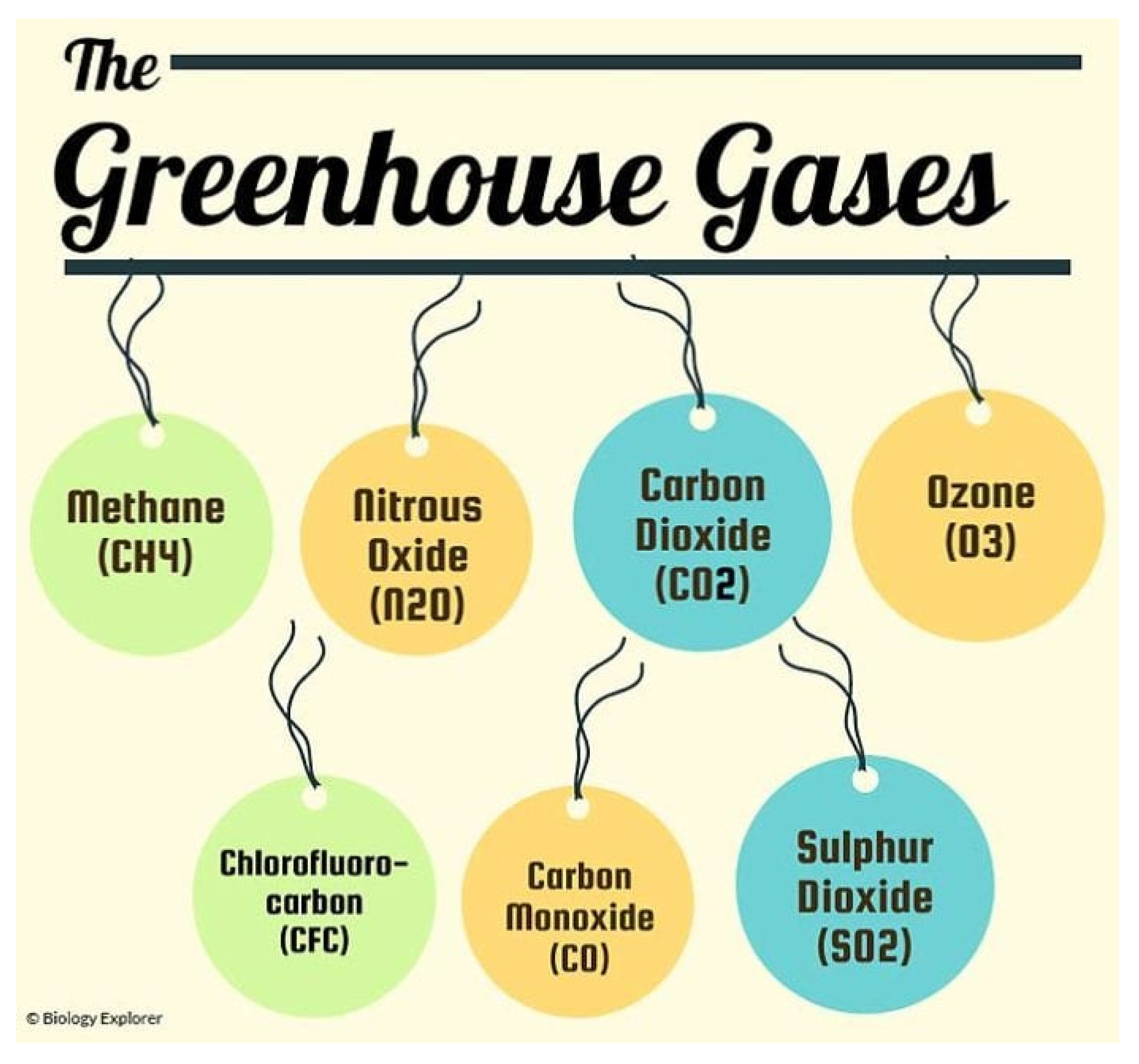
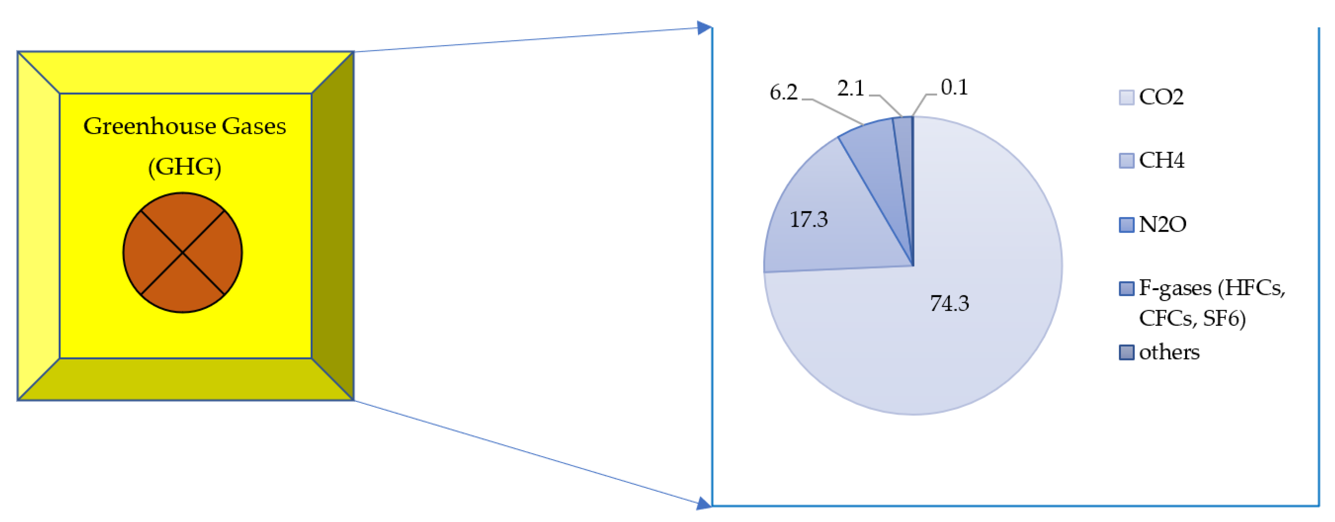
:1. Introduction
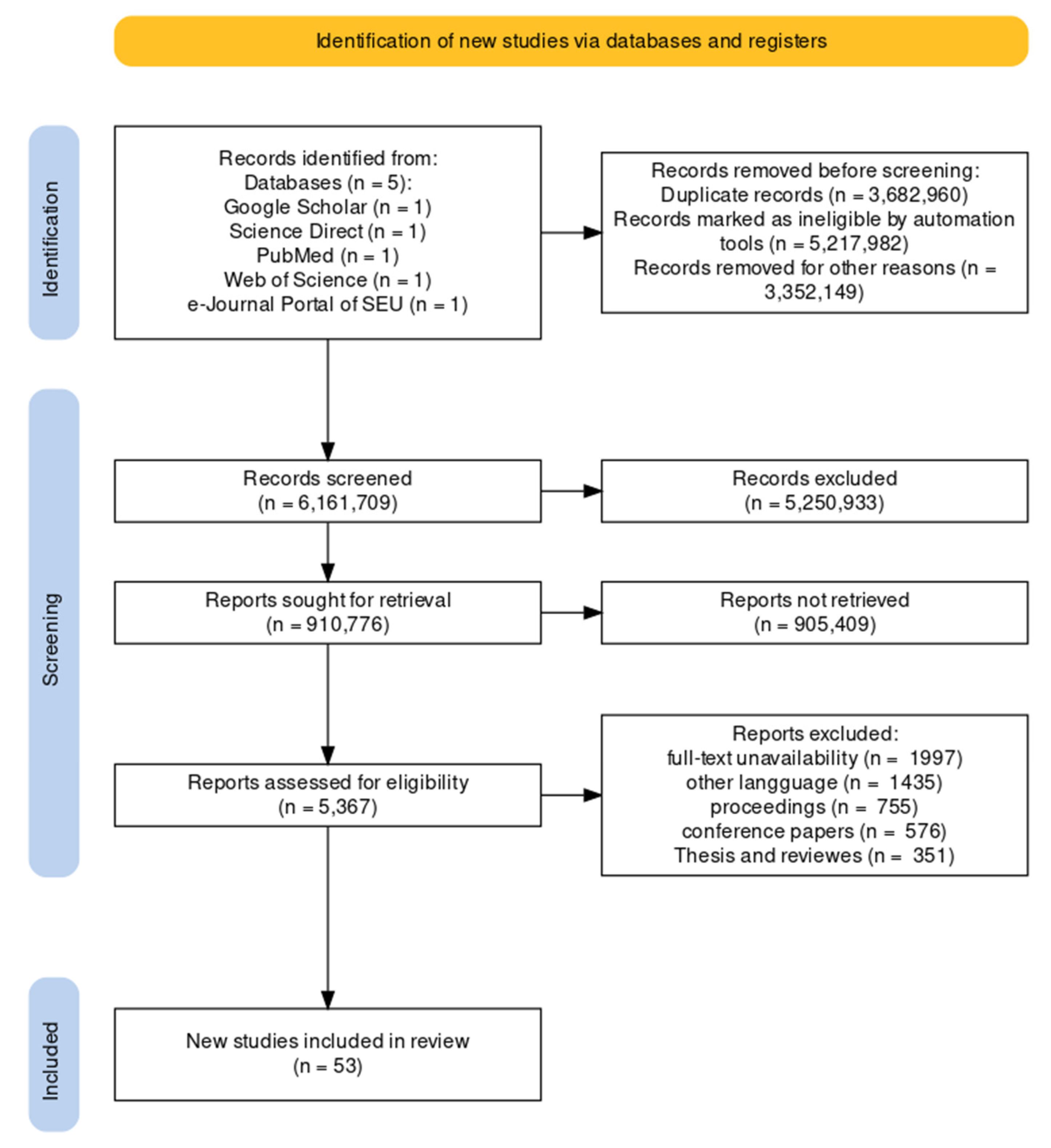
2. Methodology
- (1)
- Data source: Google Scholar, Science Direct, PubMed, Clarivate Analytics Web of Science databases, and e-Journal Portal of Southeast University (SEU) were used with the following title/keywords (no. of strings): GHG emission (446,000); CO2 emissions (2,920,000); CO2 emissions methods (2,340,000); CO2 reduction (5,070,000); GHG transportation (745,000); GHG emissions through remote sensing (RS) and GIS (18,100); GHG policy implications (753,000); GHG mitigation and challenges (365,000); CO2 emissions in Asian countries (179,000); CO2 emission from transportation (751,000); low carbon cities (2,840,000); sustainable development (3,790,000); transportation CO2 emissions monitoring and low carbon city policies (78,800).
- (2)
- Article screening: Records found in the searched databases that were duplicates or irrelevant, that did not have full-text availability, or that were inaccessible or written in languages other than English were excluded and removed from the identified records.
- (3)
- Article inclusion: Only relevant and suitable articles that discussed GHG and CO2 emissions were included.
3. Framework of CO2 Emissions from Past Studies
3.1. CO2 Emissions from Transport Sector
3.2. CO2 Emission Measurements
3.2.1. Commonly Used Methods Based on Dataset Type

| Studies | DTM | FCM | VSM | VTM | AQMM |
|---|---|---|---|---|---|
| Aksoy et al. [32] | Y/A | Y/A | Y/A | Y/A | N/A |
| Asian Development Bank [26] | Y/A | Y/A | Y/A | Y/A | N/A |
| Bhautmage et al. [37] | Y/A | N/A | N/A | Y/A | N/A |
| Chang and Lin [8] | Y/A | Y/A | N/A | N/A | N/A |
| Ding et al. [38] | N/A | Y/A | N/A | N/A | N/A |
| Faiz et al. [39] | Y/A | Y/A | Y/A | Y/A | N/A |
| Goodchild et al. [40] | Y/A | N/A | N/A | Y/A | N/A |
| Grote et al. [33] | Y/A | Y/A | Y/A | Y/A | N/A |
| Illic et al. [27] | Y/A | Y/A | N/A | N/A | N/A |
| Li et al. [18] | N/A | Y/A | Y/A | N/A | N/A |
| Saighani and Sommer [22] | N/A | Y/A | N/A | N/A | N/A |
| Singleton [41] | Y/A | N/A | N/A | Y/A | N/A |
| Shu et al. [42] | Y/A | N/A | N/A | N/A | N/A |
| Sukor et al. [15] | Y/A | Y/A | N/A | Y/A | N/A |
| Tarulescu et al. [31] | N/A | Y/A | N/A | N/A | N/A |
| Wang et al. [43] | N/A | Y/A | N/A | N/A | N/A |
| Wei and Pan [30] | Y/A | Y/A | N/A | N/A | N/A |
| Clements et al. [36] | N/A | N/A | N/A | N/A | Y/A |
| Yuan-yuan et al. [28] | Yes | Y/A | N/A | N/A | N/A |
| Zhang et al. [21] | N/A | Y/A | N/A | N/A | N/A |
| Obanya et al. [25] | N/A | N/A | N/A | N/A | Y/A |
| Zhuang et al. [44] | N/A | Y/A | N/A | N/A | N/A |
| Rusbintardjo et al. [45] | N/A | N/A | N/A | N/A | Y/A |
3.2.2. Method Selection and Comparison Based on Available Parameters
3.2.3. CO2 Emission Estimation Based on GIS/RS and Other Applications
3.3. Summary of Conducted Systematic Literature Review (SLR)
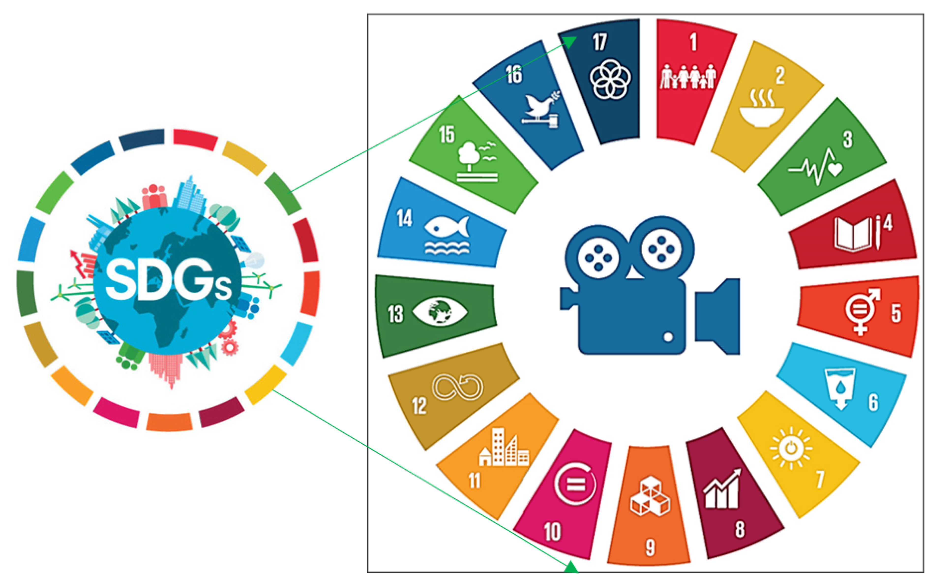
4. Transportation Sustainability and Development Programs
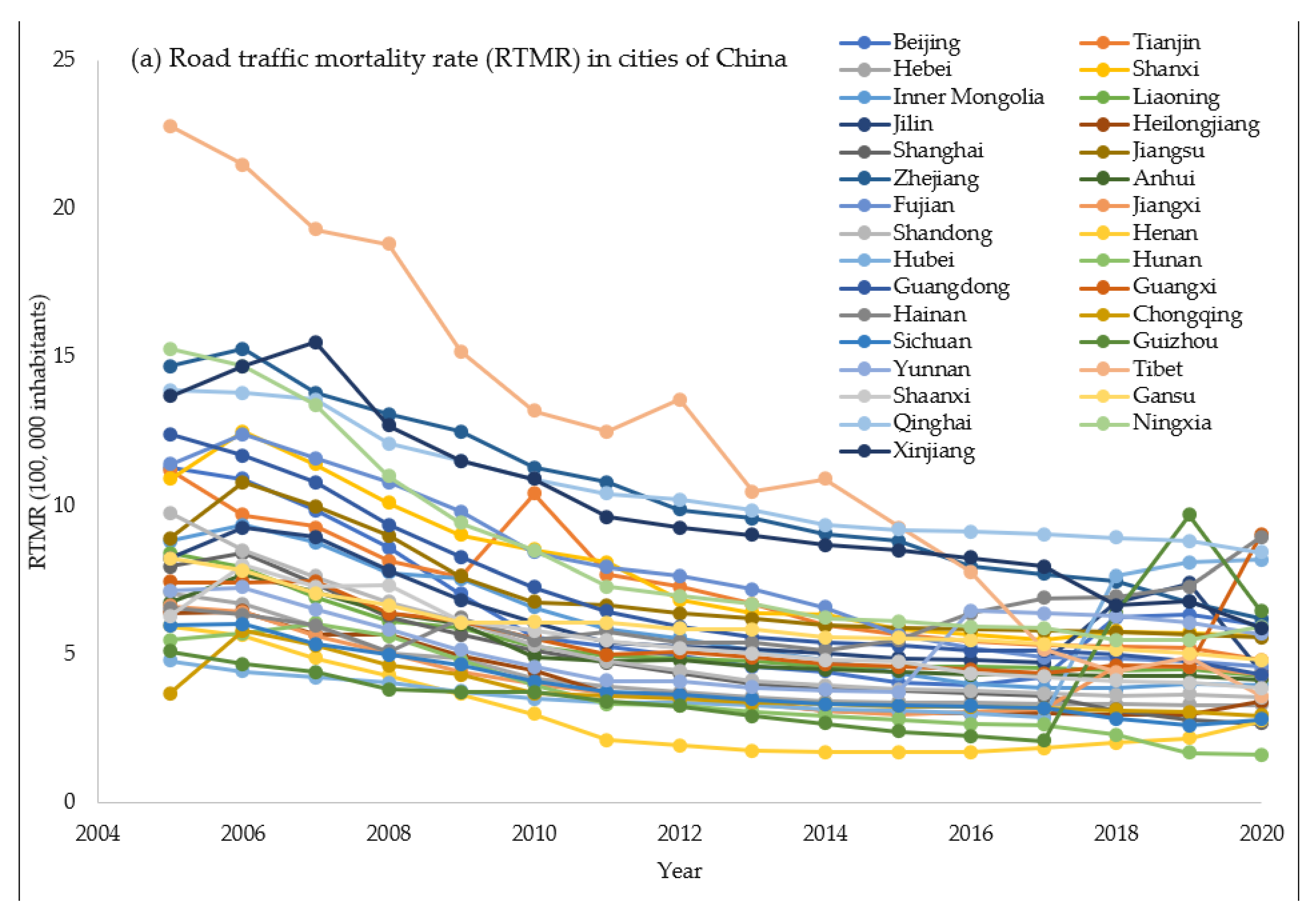
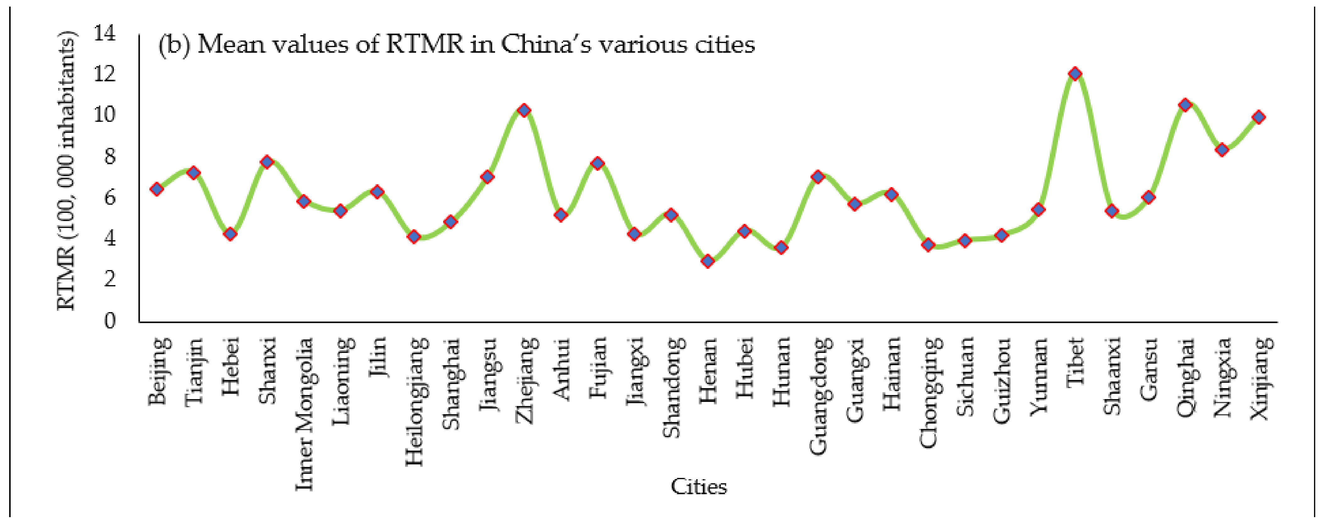
Road Traffic Mortality Rate (RTMR) in China
5. Conclusions and Future Work
Author Contributions
Funding
Institutional Review Board Statement
Informed Consent Statement
Data Availability Statement
Acknowledgments
Conflicts of Interest
References
- Environment Quality Act (Amendment 2012). Environmental Quality Act; Pencetakan Nasioanal Malaysia Berhad: Kuala Lumpur, Malaysia, 2012; Available online: https://www.ecolex.org/details/legislation/environmental-quality-amendment-act-2012-lex-faoc159115/ (accessed on 3 December 2019).
- BioExplorer.net. Explore Types of Greenhouse Gases as Agents of Climate Change. Bio Explorer. Available online: https://www.bioexplorer.net/greenhouse-gases.html/ (accessed on 31 January 2023).
- United States Environmental Protection Agency. Greenhouse Gas Emissions. 2019. Available online: https://www.epa.gov/ghgemissions/overview-greenhouse-gases (accessed on 3 December 2019).
- Masson-Delmotte, V.; Zhai, P.; Pörtner, H.-O.; Roberts, D.; Skea, J.; Shukla, P.R.; Pirani, A.; Moufouma-Okia, W.; Péan, C.; Pidcock, R. Warming of 1.5 °C above Pre-Industrial Levels and Related Global Greenhouse Gas Emission Pathways, in the Context of Strengthening the Global Response to the Threat of Climate Change, Sustainable Development, and Efforts to Eradicate Poverty. Intergovernmental Panel on Climate Change. Available online: https://www.ipcc.ch/site/assets/uploads/sites/2/2019/06/SR15_Full_Report_High_Res.pdf (accessed on 12 January 2023).
- Olivier, J.G.; Peters, J.A.H.W. Trends in Global CO2 and Total Emission Greenhouse Gas Emissions: 2018 Report; PBL Netherlands Environmental Assessment Agency: The Hague, The Netherlands, 2018; pp. 1–53. [Google Scholar]
- Olajire, A.A.; Azeez, L.; Oluyemi, E.A. Chemosphere Exposure to hazardous air pollutants along Oba Akran road, Lagos–Nigeria. Chemosphere 2011, 84, 1044–1051. [Google Scholar] [CrossRef]
- Uning, R.; Latif, M.T.; Othman, M.; Juneng, L.; Hanif, N.M.; Nadzir, M.S.M.; Maulud, K.N.A.; Jaafar, W.S.W.M.; Said, N.F.S.; Ahamad, F.; et al. A review of Southest Asian Oil Palm and Its CO2 Fluxes. Sustainability 2020, 12, 5077. [Google Scholar] [CrossRef]
- Chang, C.; Lin, T.-P. Estimation of Carbon Dioxide Emissions Generated by Building and Traffic in Taichung City. Sustainability 2018, 10, 112. [Google Scholar] [CrossRef] [Green Version]
- Inoue, T.; Yamada, K. Economic Evaluation toward Zero CO2 Emission Power Generation after 2050 in Japan. Energy Procedia 2017, 142, 2761–2766. [Google Scholar] [CrossRef]
- Shah, R.M.; Yunus, R.M.; Kadhum, A.A.H.; Yin, W.W.; Minggu, L.J. Kajian Fotomangkin Berasaskan Grafin untuk Penurunan Karbon Dioksida. J. Kejuruter. 2018, 30, 19–32. [Google Scholar]
- Mahmud, M.; Llah, I.H.A. Pencemaran Udara di Bukit Rambai, Melaka Sewaktu Peristiwa Jerebu Tahun 2005. Geogr. Malays. J. Soc. Space 2010, 6, 30–39. [Google Scholar]
- Schroder, M.; Cabral, P. Computers, Environment and Urban Systems Eco-friendly 3D-Routing: A GIS Based 3D-Routing-Model to Estimate and Reduce CO2-Emissions of Distribution transports. Comput. Environ. Urban Syst. 2019, 73, 40–55. [Google Scholar] [CrossRef] [Green Version]
- Statista Portal. Per Capita Greenhouse Gas Emissions from the Transportation Industry Worldwide in 2017, by Select Country; Energy & Environmental Services: Hamburg, Germany, 2019; Available online: https://www.statista.com/statistics/388081/global-nickel-consumption-projection/ (accessed on 3 December 2019).
- The World Bank. The Low Carbon City Development Program (LCCDP) Guidebook: A Systems Approach to Low Carbon Development in Cities; The World Bank: Washington, DC, USA, 2014; pp. 1–82. [Google Scholar]
- Sukor, N.S.A.; Basri, N.K.; Hassan, S.A. Carbon Footprint Reduction in Transportation Activity by Emphasizing the Usage of Public Bus Services among Adolescents. IOP Conf. Ser. Mater. Sci. Eng. 2017, 226, 1–8. [Google Scholar] [CrossRef] [Green Version]
- Transport & Environment. CO2 Emissions from Cars: The Facts. 2018. Available online: https://www.transportenvironment.org/publications/CO2-emissions-cars-facts (accessed on 3 December 2019).
- Mickunaitis, V.; Pikunas, A.; Mackoit, I. Reducing Fuel Consumption and CO2 Emission in Motor Cars. Transport 2007, 22, 160–163. [Google Scholar] [CrossRef] [Green Version]
- Li, J.; Lu, Q.; Fu, P. Carbon Footprint Management of Road Freight Transport under the Carbon Emission Trading Mechanism. Math. Probl. Eng. 2015, 2015, 814527. [Google Scholar] [CrossRef]
- Santos, G. Road transport and CO2 emissions: What are the challenges? Transp. Policy 2017, 59, 71–74. [Google Scholar] [CrossRef]
- Bharadwaj, S.; Ballare, S.; Chandel, M.K. Impact of Congestion on Greenhouse Gas Emissions for Road Transport in Mumbai Metropolitan Region. Transp. Res. Procedia 2017, 25, 3538–3551. [Google Scholar] [CrossRef]
- Zhang, K.; Batterman, S.; Dion, F. Vehicle emissions in congestion: Comparison of work zone, rush hour and free-flow conditions. Atmos. Environ. 2011, 45, 1929–1939. [Google Scholar] [CrossRef]
- Saighani, A.; Sommer, C. Potentials for Reducing Carbon Dioxide Emissions and Conversion of Renewable Energy for the Regional Transport Market—A Case Study. Transp. Res. Procedia 2017, 25, 3479–3494. [Google Scholar] [CrossRef]
- Gharineiat, Z.; Khalfan, M. Using the Geographic Information System (GIS) in the Sustainable Transportation. Int. J. Civ. Archtectural Eng. 2011, 5, 1425–1431. [Google Scholar]
- Kan, Z.; Tang, L. Estimating Vehicle Fuel Consumption and Emissions Using GPS Big Data. Int. J. Environ. Res. Public Health 2018, 15, 566. [Google Scholar] [CrossRef] [Green Version]
- Obanya, H.E.; Amaeze, N.H.; Togunde, O.; Otitoloju, A.A. Air Pollution Monitoring Around Residential and Transportation Sector Locations in Lagos Mainland. J. Health Pollut. 2018, 8, 180903. [Google Scholar] [CrossRef] [Green Version]
- Asian Development Bank. Reducing Carbon Emissions from Transport Projects; Independent Evaluation Department: Metro Manila, PH, USA, 2010. [Google Scholar]
- Illic, I.; Vukovic, M.; Strbac, N.; Urosevic, S. Applying GIS to Control Transportation Air Pollutants. Pol. J. Environ. Stud. 2014, 23, 1849–1860. [Google Scholar]
- Liu, Y.-Y.; Wang, Y.-Q.; An, R.; Li, C. The Spatial Distribution of Commuting CO2 Emissions and the Influential Factors: A Case Study in Xi’an, China. Adv. Clim. Chang. Res. 2015, 6, 46–55. [Google Scholar] [CrossRef]
- Velaquez, L.; Munguia, N.E.; Will, M.; Zavala, A.G.; Verdugo, S.P.; Delakowitz, B.; Giannetti, B. Sustainable Transportation Strategies for Decoupling Road Vehicle Transport and Carbon Dioxide Emissions. Manag. Environ. Qual. Int. J. 2015, 26, 373–388. [Google Scholar] [CrossRef] [Green Version]
- Wei, P.; Pan, H. Research on Individual Carbon Dioxide Emissions of Commuting in Peri-Urban Area of Metropolitan Cities Peri-Urban Area of Metropolitan Cities—An Empirical Study in Shanghai. Transp. Res. Procedia 2017, 25, 3459–3478. [Google Scholar] [CrossRef]
- Tarulescu, S.; Tarulescu, R.; Soica, A.; Leahu, C.I. Smart Transportation CO2 Emission Reduction Strategies. IOP Conf. Ser. Mater. Sci. Eng. 2017, 252, 012051. [Google Scholar] [CrossRef] [Green Version]
- Aksoy, A.; Kucukoglu, I.; Ene, S.; Ozturk, N. Integrated Emission and Fuel Consumption Calculation Model for Green Supply Chain Management. Procedia Soc. Behav. Sci. 2014, 109, 1106–1109. [Google Scholar] [CrossRef] [Green Version]
- Grote, M.; Williams, I.; Preston, J.; Kemp, S. Including congestion effects in urban road traffic CO2 emissions modelling: Do Local Government Authorities have the right options? Transp. Res. Part D 2016, 43, 95–106. [Google Scholar] [CrossRef] [Green Version]
- Toffolo, S.; Morello, E.; Rocco, D.; Di Valdes, C.; Punzo, V. ICT—Emissions Deliverable 2.1: Methodology; Garcia-castro, A., Vouitsis, I., Ntziachristos, L., Samaras, Z., Eds.; European Commission: Brussels, Belgium, 2013. [Google Scholar]
- Xie, X.; Semanjski, I.; Gautama, S.; Tsiligianni, E. A Review of Urban Air Pollution Monitoring and Exposure Assessment Methods. Int. J. Geo-Inf. 2017, 6, 389. [Google Scholar] [CrossRef] [Green Version]
- Clements, A.L.; Griswold, W.G.; Rs, A.; Johnston, J.E.; Herting, M.M.; Thorson, J.; Collier-oxandale, A.; Hannigan, M. Low-Cost Air Quality Monitoring Tools: From Research to Practice (A Workshop Summary). Sensors 2017, 11, 2478. [Google Scholar] [CrossRef] [Green Version]
- Bhautmage, U.P.; Tembhurkar, A.R.; Sable, A.; Sinha, S.; Adarsh, S. Carbon Footprint for Transportation Activities of an Institutional Campus. J. Energy Environ. Carbon Credit. 2015, 5, 9–19. [Google Scholar]
- Ding, J.; Jin, F.; Li, Y.; Wang, J. Analysis of Transportation Carbon Emissions and Its Potential for Reduction in China. Chin. J. Popul. Resour. Environ. 2013, 11, 17–25. [Google Scholar] [CrossRef] [Green Version]
- Faiz, A.; Weaver, C.S.; Walsh, M.P. Air Pollution from Motor Vehicles: Standard and Technologies for Controlling Emissions; World Bank Group: Washington, DC, USA, 1996. [Google Scholar]
- Goodchild, A.; Wygonik, E.; Mayes, N.; Mayes, N. An analytical model for vehicle miles traveled and carbon emissions for goods delivery scenarios. Eur. Transp. Res. Rev. 2018, 10, 1–10. [Google Scholar] [CrossRef]
- Singleton, A. A GIS Approach to Modelling CO2 Emissions Associated with the Pupil School Commute. Int. J. Geogr. Inf. Sci. 2014, 28, 256–273. [Google Scholar] [CrossRef] [Green Version]
- Shu, Y.; Lam, N.S.N.; Reams, M.; Rouge, B. A New Method for Estimating Carbon Dioxide Emission from Transportation at Fine Spatial Scales. Environ. Res. Lett. 2010, 5, 1–19. [Google Scholar] [CrossRef] [PubMed]
- Wang, T.; Li, H.; Zhang, J.; Lu, Y. Influencing Factors of Carbon Emission in China’s Road Freight Transport. Procedia-Soc. Behav. Sci. 2012, 43, 54–64. [Google Scholar] [CrossRef] [Green Version]
- Zhuang, X.; Jiang, K.; Zhao, X. Analysis of the Carbon Footprint and Its Environmental Impact Factors for Living and Travel in Shijiazhuang City. Adv. Clim. Chang. Res. 2011, 2, 159–165. [Google Scholar] [CrossRef]
- Rusbintardjo, G.; Jiun, C.M.; Ibrahim, A.N.H.; Babashamsi, P.; Yusoff, N.I.M.; Hainin, M.R. A Comparative Study of Monitoring Methods in Sustainable Pevement System Development. J. Teknol. 2019, 81, 41–51. [Google Scholar]
- Raje, F.; Tight, M.; Pope, F.D. Traffic pollution: A search for solutions for a city like Nairobi. Cities 2018, 82, 100–107. [Google Scholar] [CrossRef]
- TRANSCAT Portal. Understanding Air Quality Test Instruments. Available online: https://www.transcat.com/calibration-resources/application-notes/air-quality-measurement/ (accessed on 22 May 2020).
- Chae, B.; Yang, C.; Olson, D.; Sheu, C. The impact of advanced analytics and data accuracy on operational performance: A contingent resource based theory (RBT) perspective. Decis. Support Syst. 2014, 59, 119–126. [Google Scholar] [CrossRef] [Green Version]
- Fortin, J.A.; Cardille, J.A.; Perez, E. Multi-sensor Detection of Forest-cover Change across 45 years in Mato Grasso, Brazil. Remote Sens. Environ. 2020, 238, 111266. [Google Scholar] [CrossRef]
- Byrne, E.; Donnely, E. Carbon Emissions, Transport and Location: A Sustainability Toolkit for Stakeholders in Development. In Proceedings of the Irish Transport Network 2012 Conference, University of Ulster, Belfast, UK, 9–30 August 2012; pp. 1–9. [Google Scholar]
- Asdrubali, F.; Presciutti, A.; Scrucca, F. Development of a greenhouse gas accounting GIS-based tool to support local policy making—Application to an Italian municipality. Energy Policy 2013, 61, 587–594. [Google Scholar] [CrossRef]
- Dalumpines, R. Using RS and GIS in Developing Indicators to Support Urban Transport Ecological Footprint Analysis: The Case of Ahmedabad City, India; International Institute for Geo-Information Science and Earth Observation Enschede: Enschede, The Netherlands, 2008. [Google Scholar]
- Chen, S.; Crawford, R.H. Modeling the Carbon Footprint of Urban Development: A Case Study in Melbourne. In Living and Learning: Research for a Better Built Environment: 49th International Conference of the Architectural Science Association, 2–4 December 2015, Melbourne, Australia; The Architectural Science Association and The University of Melbourne: Melbourne, Australia, 2015; pp. 267–277. [Google Scholar]
- Yazid, M.R.M.; Baharin, N.I.K.; Yaacob, N.F.F. A Study of Reducing Carbon Footprint towards the Sustainability Campus. In Proceedings of the International Conference on Education, Islamic Studies and Social Sciences Research 2019, Medan North Sumatra, Indonesia, 2–3 September 2019; pp. 1–11. [Google Scholar]
- Yousefi-sahzabi, A.; Sasaki, K.; Djamaluddin, I.; Yousefi, H.; Sugai, Y. GIS modeling of CO2 Emission Sources and Storage Possibilities. Energy Procedia 2011, 4, 2831–2838. [Google Scholar] [CrossRef] [Green Version]
- Idris, N.; Mahmud, M. Kajian Jejak Karbon di Kuala Lumpur. J. Soc. Sci. Humanit. 2017, 12, 165–182. [Google Scholar]
- Lorena, A.; Albert, M.; Maria, D. Carbon Footprint Analysis: Towards a Projects Evaluation Model for Promoting Sustainable Development. Procedia Econ. Financ. 2013, 6, 353–363. [Google Scholar]
- Ma, F.; Wang, W.; Sun, Q.; Liu, F.; Li, X. Ecological Pressure of Carbon Footprint in Passenger Transport: Spatio-Temporal Changes and Regional Disparities. Sustainability 2018, 10, 317. [Google Scholar] [CrossRef] [Green Version]
- Eleventh Malaysia Plan. In Eleventh Malaysia Plan (2016–2020); Economic Planning Unit, Prime Minister’s Department: Kuala Lumpur, Malaysia, 2016.
- Yaacob, N.F.F. Spatial Relationship between Road Characteristics and Environmental Factors towards Road Accident in Kedah; Universiti Teknologi MARA: Kuala Lumpur, Malaysia, 2019. [Google Scholar]
- World Health Organization (WHO). Global Status Report on Road Safety. Available online: https://www.who.int/violence_injury_prevention/road_safety_status/2018/en/ (accessed on 24 January 2020).
- National Transport Policy (NTP). National Transport Policy 2019–2030; Ministry of Transport Malaysia: Putrajaya, Malaysia, 2019. [Google Scholar]
- SCOOP Portal. Industry 4.0: The Fourth Industrial Revolution—Guide to Industry 4.0. 2020. Available online: https://www.i-scoop.eu/industry-4-0/ (accessed on 3 December 2019).
- Kanniah, K.D. Low Carbon Society Blueprint for ISkandar Malaysia 2025; UTM-Low Carbon Asia Research Center: Johor Bahru, Malaysia, 2013. [Google Scholar]
- Adnan, A.S. My100, My50 Lonjak 40 Peratus Pengguna rel, Bas Prasarana; Berita Harian Online: Kuala Lumpur, Malaysia. Available online: https://www.bharian.com.my/berita/nasional/2019/05/567349/my100my50-lonjak-14-peratus-pengguna-rel-bas-prasarana (accessed on 24 January 2020).
- GreenTech Malaysia. Low Carbon Mobility; GreenTech Malaysia Portal: Selangor, Malaysia, 2019; Available online: https://www.greentechmalaysia.my/our-services/low-carbon-mobility/ (accessed on 24 January 2020).
- ASEAN Jakarta. Sustainable Land Transport Indicators on Energy Efficiency and Greenhouse Gas Emissions in ASEAN—Guidelines; ASEAN Secretariat: Jakarta, Indonesia, 2021. [Google Scholar]


| Author | Studied Region | Analytical Tool Used | Output | |
|---|---|---|---|---|
| Region | Area | |||
| Asdrubali et al. [51] | Italy | Spoleto | GIS modeling | GHG or CO2 emission |
| Bharadwaj et al. [20] | India | Mumbai | VKT, FCM | |
| Byrne and Donnely [50] | Ireland | Greater Dublin Area | GIS modeling | |
| Chen and Crawford [53] | Australia | Melbourne | GIS and RS modeling; Malaysian smart grid | |
| Dalumpines [52] | India | Ahmedabad | GIS and RS modeling | |
| Ding et al. [38] | China | LMDI method | ||
| Grote et al. [33] | United Kingdom | Southampton | traffic variable emissions models | |
| Idris and Mahmud [56] | Malaysia | Kuala Lumpur | CFA model | |
| Illic et al. [27] | Europe | Serbia | GIS modeling, mathematical sub-models (COPERT IV, CALINE3) | |
| Lorena et al. [57] | Europe | Bucharest, Romania | CFA model | |
| Ma et al. [58] | China | 8 economic zones | ArcGIS and GeoDa software | |
| Schroder and Cabral [12] | Portugal | Lisbon | GIS, 3D-Routing-and DEM model | |
| Shu et al. [42] | USA | State of Louisiana | ArcGIS 9.2, distance-decay principle | |
| Tarulescu et al. [31] | Europe | Ghimbav City | mathematical model, vehicle fleet renewal, RAT Brasov | |
| Wang et al. [43] | China | Beijing | PLSR method | |
| Yazid et al. [54] | Indonesia | Sumatra | CFA model | |
| Yousefi-sahzabi et al. [55] | Japan | Fukuoka | GIS modeling and mapping, prediction dispersion model | |
| Yuan-yuan et al. [28] | China | Xian | correlation analysis and spatial model | |
| Zhang et al. [21] | USA | Michigan | CMEM (MOBILE6.2) | |
| Zhuang et al. [44] | China | Shijiazhuang City | CFA model | |
Disclaimer/Publisher’s Note: The statements, opinions and data contained in all publications are solely those of the individual author(s) and contributor(s) and not of MDPI and/or the editor(s). MDPI and/or the editor(s) disclaim responsibility for any injury to people or property resulting from any ideas, methods, instructions or products referred to in the content. |
© 2023 by the authors. Licensee MDPI, Basel, Switzerland. This article is an open access article distributed under the terms and conditions of the Creative Commons Attribution (CC BY) license (https://creativecommons.org/licenses/by/4.0/).
Share and Cite
Zubair, M.; Chen, S.; Ma, Y.; Hu, X. A Systematic Review on Carbon Dioxide (CO2) Emission Measurement Methods under PRISMA Guidelines: Transportation Sustainability and Development Programs. Sustainability 2023, 15, 4817. https://doi.org/10.3390/su15064817
Zubair M, Chen S, Ma Y, Hu X. A Systematic Review on Carbon Dioxide (CO2) Emission Measurement Methods under PRISMA Guidelines: Transportation Sustainability and Development Programs. Sustainability. 2023; 15(6):4817. https://doi.org/10.3390/su15064817
Chicago/Turabian StyleZubair, Muhammad, Shuyan Chen, Yongfeng Ma, and Xiaojian Hu. 2023. "A Systematic Review on Carbon Dioxide (CO2) Emission Measurement Methods under PRISMA Guidelines: Transportation Sustainability and Development Programs" Sustainability 15, no. 6: 4817. https://doi.org/10.3390/su15064817