Article

Simulation of Water Balance Components Using SWAT Model at Sub Catchment Level

by
Dinagarapandi Pandi
,
Saravanan Kothandaraman
* and
Mohan Kuppusamy
School of Civil Engineering, Vellore Institute of Technology, Chennai 600127, India
*
Author to whom correspondence should be addressed.
Sustainability 2023, 15(2), 1438; https://doi.org/10.3390/su15021438
Submission received: 25 July 2022 / Revised: 4 December 2022 / Accepted: 15 December 2022 / Published: 12 January 2023

Abstract

:
Simulation of Water Balance Components (WBCs) is import for sustainable water resources development and management. The Soil Water and Assessment Tool (SWAT) is a semi-distributed hydrological model to estimate the WBCs by forcing the hydrological response unit (HRU) and meteorological variables. The developed model simulates five WBCs viz. surface runoff, lateral flow, percolation, actual evapotranspiration and soil water at sub catchment level. To demonstrate the model compatibility a case study taken over Chittar catchment, Tamilnadu, India. The catchment was divided in to 11 sub catchments. The ten year interval LULC (i.e., 2001 and 2011), twenty year daily meteorological data (i.e., 2001–2020) and time invariant soil and slope data were used in developing the water balance model. Developed model was calibrated and evaluated with river gauge monthly discharging using SUFI-2 algorithm in SWAT-CUP. The model calibration performed in two stage i.e., pre-calibration (2001–2003) and post-calibration (2004–2010). The model performance was evaluated with unseen river gauge discharging data (i.e., 2011–2015). Then, results of statistical outputs for the model were coefficient of determination (R2) is 0.75 in pre-calibration, 0.94 in post-calibration and 0.81 in validation. Further strengthen the model confidential level the sub catchments level monthly actual evapotranspiration were compared with gridded global data GLEAM v3.6a. Finally, the developed model was simulate the five WBCs whereas, surface runoff, lateral flow, percolation, actual evapotranspiration and soil water at sub catchment level during 2001–2020. The sub catchment level WBCs trend helps to make fast and accurate decision. At all 11 sub catchments a long drought was observed during 2016–2018 due to failure of northeast monsoon. The WBCs were directly reinforced by their north east monsoon which gives the major portion of rainfall i.e., September to December. Hence all the WBCs were directly correlated with rainfall with or without time lag. By understanding the sub catchment level of monthly WBCs over the Chittar catchment is useful for land and water resource management.

1. Introduction

A major threat to survival of living beings over developing nations in the 21st century is water scarcity. The rising population and mismanagement of water resource lead to water scarcity. Thereby, hydro meteorological phenomenon such as uneven distribution of rainfall and soil water content (SW) that contributes on a large scale to water scarcity [1,2], so it resolves by an understanding of hydrological responses. At regional scale, SW is a limiting factor in crop production as crop water required often exceeds rainfall or irrigation. Hydrological responses are the rainfall event that responds to form surface and subsurface flow in the catchment. Surface and subsurface flow tells about the runoff, infiltration, SW, interception, depression storage and percolation happen in the catchment by considering evaporation and transpiration. These hydrological responses driving the surface and subsurface water thus it is called as water balance components (WBCs). Catchment is an area of land where all the rain water collected and drains into lowest elevation point after meeting abstraction [3]. In tropical country like India, meteorological drought and cyclonic floods happens due to monsoon failure and retreating rainfall by the Inter Tropical Convergence Zone; gives the gain and loss of water by means of hydrological response at the catchment.
Water balance model delineate the spatiotemporal distribution of WBCs at catchment [4,5]. Generally, water balance model is purely based upon the law of conservation of mass principle; it varied from one to another form; observes from the hydrological cycle. Major components of water balance model in semi-arid regions were rainfall, actual evapotranspiration (AE), runoff, infiltration, SW etc. applied in the model development as spatially and temporal according to their dynamic hydrological behavior in the catchments [6,7,8,9]. From the WBCs, accessibility of a component was carried as unknown, and known component gives the results for the unknown component at certain time interval. As per temporal basis, water balance model can be classified as daily, monthly, seasonal and annually. The monthly and annual scale models are more suitable for water resources development and management. Graf and Jawgiel, [10] developed water balance model to simulate components likely evapotranspiration (ET), runoff and infiltration and resulted outcomes used in the integrated urban planning. Ali Amin et al. [11] applied water balance model for the catchment wide effective water resources management. Li et al. [12] simulated water yield by incorporating future Land Use and Land Cover (LULC) change scenarios and to estimated water yield coefficient for every LULC class. Kundu et al. [9] developed water balance model to quantify the impact of individual as well as the integrated climate and LULC changes. Garg et al. [13] evaluated the long term impact of LULC change over the WBCs. Xu and Singh, [14] had reviewed that monthly water balance model and they suggested that monthly scale model were most suitable to solve it through catchment scale of the spatial scheme. The commercial distributed water balance models include VIC-2L [15]; Wapaba model [16]; AWBM [17]; SWAT [18,19,20]; MIKE-SHE coupled MIKE-11 [21] etc. Many previous studies reported that, most of the distributed water balance models were data intensive and requires high resolution field data [22,23]. There was considerable level of uncertainty associated with model structure, boundary conditions, input parameters due to heterogeneity and data resolution. Currently, high resolution hydro meteorological data were not available in most of the developing countries like India, Indonesia, Africa, etc. Further, most of the existing commercial water balance models are very complex, extremely costly and require higher computational efforts. Accordingly, majority of existing water balance studies carried over developing countries are lumped or GIS based overlay analysis [20]. A few studies in physically distributed, water balance models were carried out with the less water balance component’s likely rainfall and ET because of limited hydrological and meteorological data [21]. Presently, free and open source remote sensing technology is emerging as a promising solution for earth and atmospheric observations due to its high spatiotemporal resolutions. This remote sensing data could be the input for developing hydrological models. Hence, open source water balance models interfaced with GIS were essential in developing countries especially in limited hydro meteorological data scenario. One such a model available for water resources professional was Soil and Water Assessment Tool (SWAT). SWAT is one of the widely applied open source semi distributed hydrological model because it gives the different results from the different platform of hydrology applications such as water balance modeling, rainfall runoff modeling, reservoir modeling, sediment yield, nutrient cycle for agricultural, etc. It can specify the model to have a lumped response at the Hydrological Response Unit (HRU) level while also being able to estimate the spatial variability at the sub catchment level. Hence no initial and boundary conditions were required for model simulation. Keep in mind that an HRU is a basic spatial unit with distinct soil, LULC, and slope conditions. After abstraction, each HRU’s runoff is sent to a stream before ending up at the catchment outflow. The present study aims to developing a general water balance model to simulate the WBCs at the catchment and sub catchment level especially under limited data. Keeping the above in view, the objectives of the present research study are envisaged as follows:
  • Developing semi distributed monthly water balance model over a catchment in south India in SWAT. Model provides the spatial and temporal distribution of WBCs viz. AE, surface runoff, lateral flow, SW and percolation over a catchment.
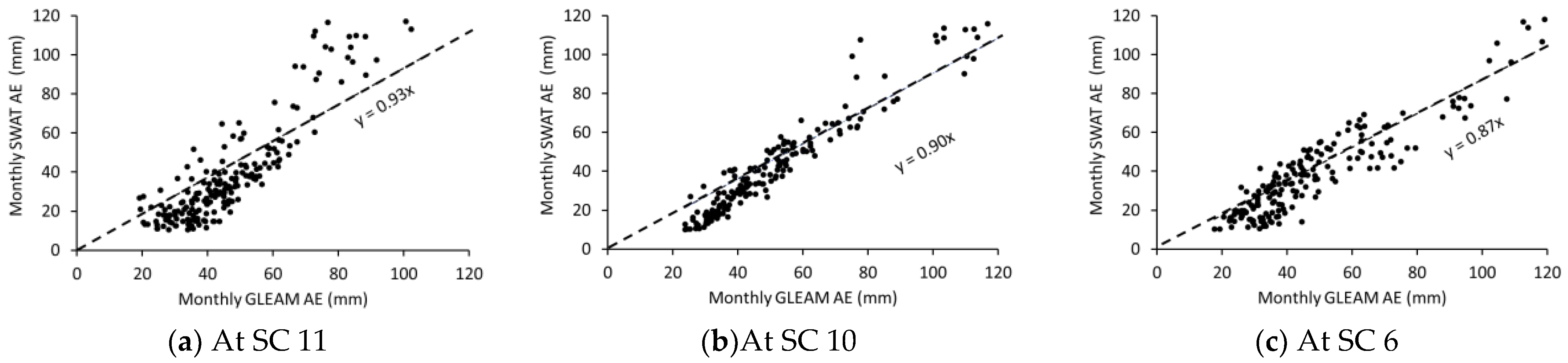
  • To evaluate the applicability and suitability, the developed model was calibrated and validated over using measured gauge discharge. Additionally, the model performance was verified with gridded global AE.
  • The calibrated model is used for spatiotemporal mapping of WBCs over the sub catchments by forcing the prevailing LULC and meteorological conditions.
To demonstrate the model application a case study was taken over Chittar catchment a tributary of Thamirabarani river basin, Tamilnadu, south India. This catchment has about 75% vegetation cover (agricultural and forest land). The semi-arid conditions over the south India include scanty rainfall, high temperature and high evaporation throughout the year. Lack of major water storage infrastructure and institutional support, monsoon rainfall is the only available source of water, especially in the catchment. Kumar et al. [12], Nithya et al. [12] and Pandi et al. [12] delineated groundwater potential zones using remote sensing and GIS based overlay analysis over the Chittar catchment. Further, over the Chittar catchment no distributed/semi distributed hydrological model studies reported in the peer reviewed journal. Hence, modelling the WBCs at catchment is vital for to address the issues associated with food security, disaster risk reduction, resilient livelihoods, water resource planning and managing, land use change analysis, urban planning, climate change, groundwater harvesting, runoff harvesting site etc.

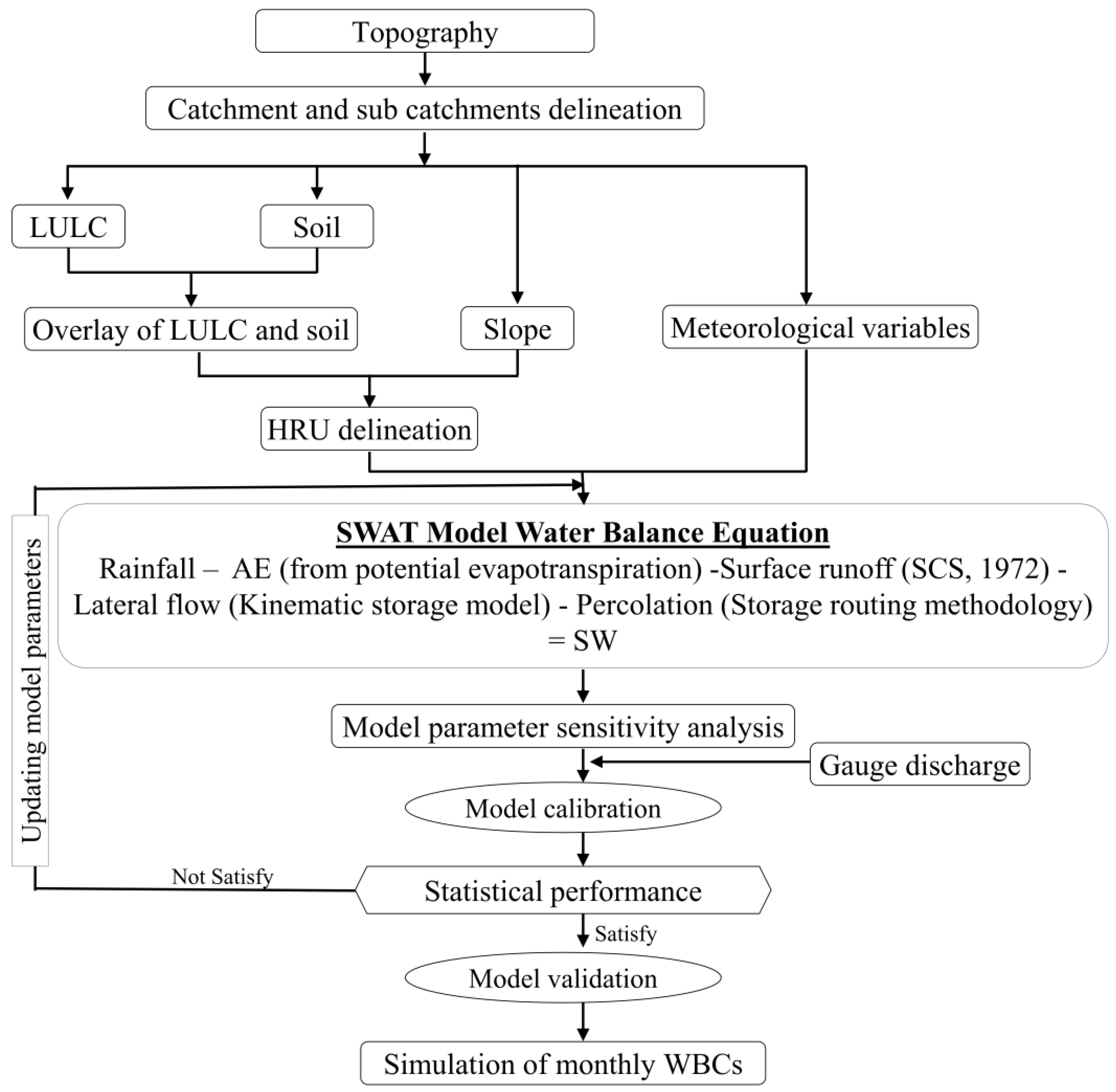
2. Materials and Methods
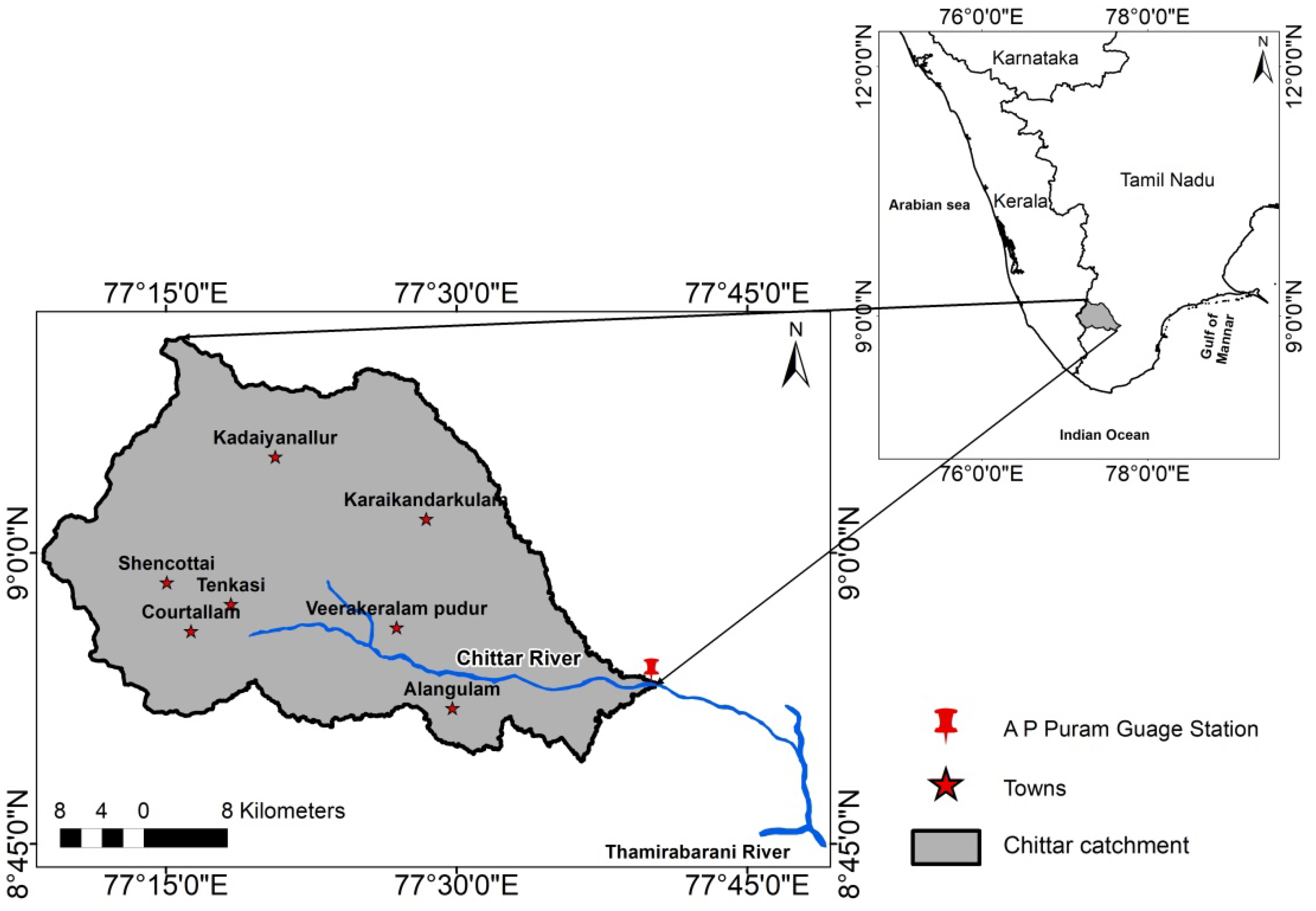
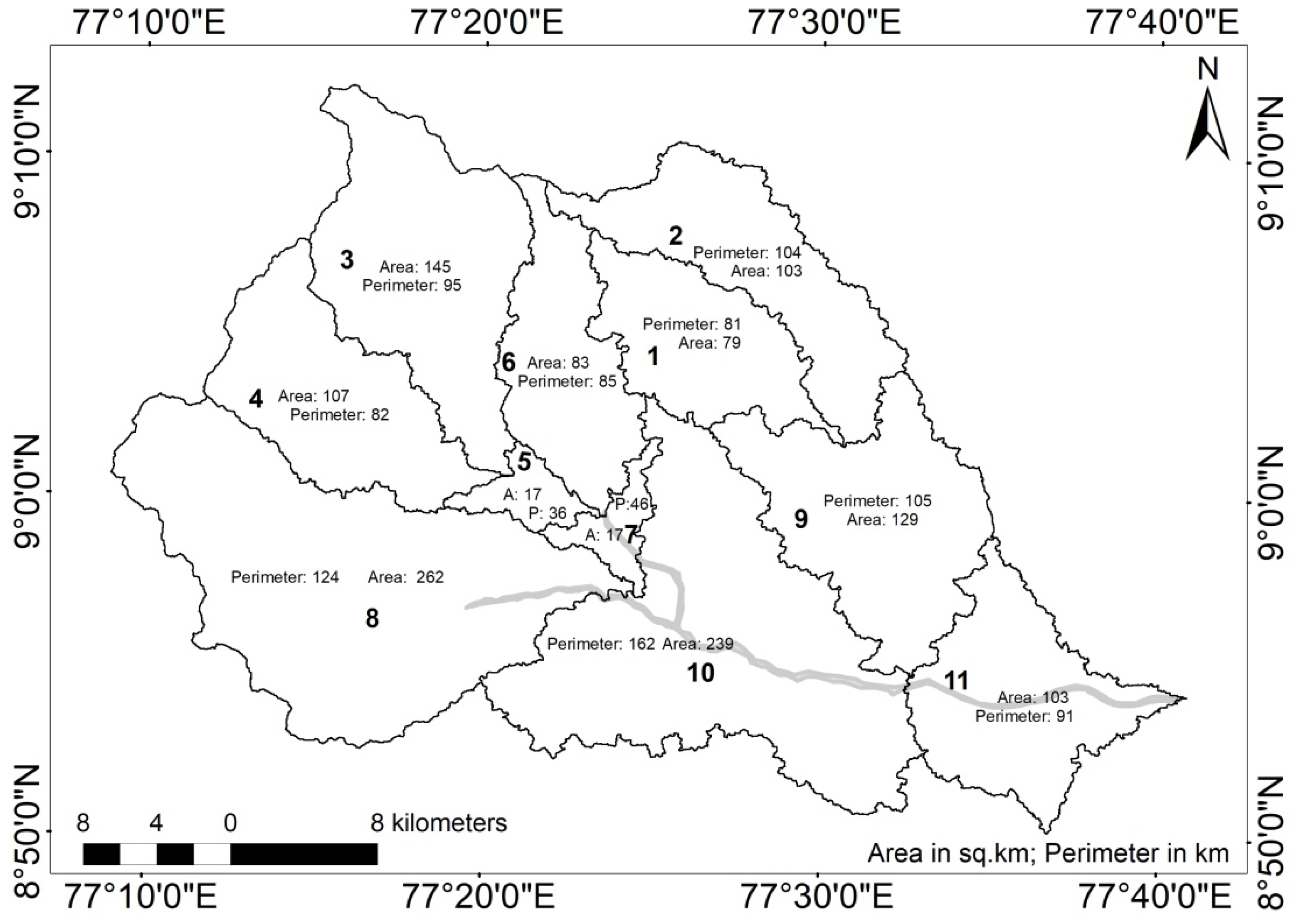
In SWAT, a catchment is divided into multiple sub catchments, which are then further subdivided into HRU that consist of unique combination land use management, slope, and soil characteristics [24]. In this study SWAT model was used to simulate the WBCs such as rainfall, AE, overland flow, lateral flow, return flow, infiltration and SW for the catchment. Input parameters were used in the model development; they were topography, LULC, soil, slope and meteorological variables. The flow chart of methodology is shown in Figure 1. In this study, Chittar catchment was divided in to 11 sub catchments with A.P Puram gauging station as outlet and five WBCs are predicted over every sub catchment.
In SWAT several algorithms that are available to simulate each WBCs [25]. The selection of the appropriate algorithm depends on purpose of study, data availability, expected accuracy, and spatiotemporal distribution of the model domain. Rainfall usually is taken from the meteorological observatory. In this study potential evapotranspiration estimated using Penman and Monteith method [26], surface runoff using Modified Soil Conservation Service Curve Number method (SCS-CN) [27], lateral flow using kinematic storage model [28] and percolation using storage routing model [29]. The AE is arrived from potential evapotranspiration by multiplying by a reduction factor which is function of leaf area index, soil depth and available SW [30]. Finally, SW was estimated by mass balance principle and showed as gain and loss parameter of the model [31]. The SW was the amount of water that lies in the soil after interacts with various WBCs. Accordingly, SW simulated in SWAT by using water balance equation as given in Figure 1. The spatiotemporal distribution of SW is important for application related to irrigation, crop yield, crop selection, climate change, land and water resources management and development. The readily available soil moisture content was arrived as difference of field capacity and welting point of respective top soil layer [32]. The output of the model provides the spatiotemporal WBCs distribution over the Chittar catchment. The surface runoff and lateral flow were routed from all HRU to sub catchment and subsequently to catchment outlet through channel network using variable storage routing method [29]. The field measured discharge at outlet was used to calibrate and validate the model. Further strengthening the model performance, simulated sub catchment level AE was also compared with the third party regional AE dataset.
During the model development influences of few small check dams and tanks over the catchment were not included in the model development. The model was calibrated with gauge discharge at the outlet of the basin and there is possibility of overfitting. Hence it is necessary to calibrating with multiple WBCs to avoid overfitting [33]. The model simulate temporal trend of five WBCs over 11 sub catchments for past twenty year period. The five WBCs temporal trend were compared visually. This twenty year simulation period is not sufficient to include extreme hydrological events. Hence forecasting of spatiotemporal distribution of WBCs by forcing hydrological and meteorological scenario is an important for planners, policy makers and researchers to make quantitative decisions.

2.1. Study Area

The Chittar river is located in Tamilnadu, south India. It is one of the major tributaries of Thamirabarani river basin. The location map of Chittar catchment is show in Figure 2. Its area spans the latitude of 8°45′ N to 9°15′ N and longitudes of 77°10′ E to 77°50′ E covers the area of about 1300 sq km. The length of the main river travels about the 82 kms reaches into the Thamirabarani river. The delineated boundaries of the 11 sub catchments are also shown in Figure 2. It lies in a hot and dry climate zone with temperature varying from 28 °C to 42 °C—April, May and early June. North east monsoon of Chittar catchment starts from the October to December receives a 50% of annual rainfall, South west monsoon starts from June to August receives a 30% of rainfall. Total annual rainfall of this catchment is about 880 mm.

2.2. Hydrological Response Unit
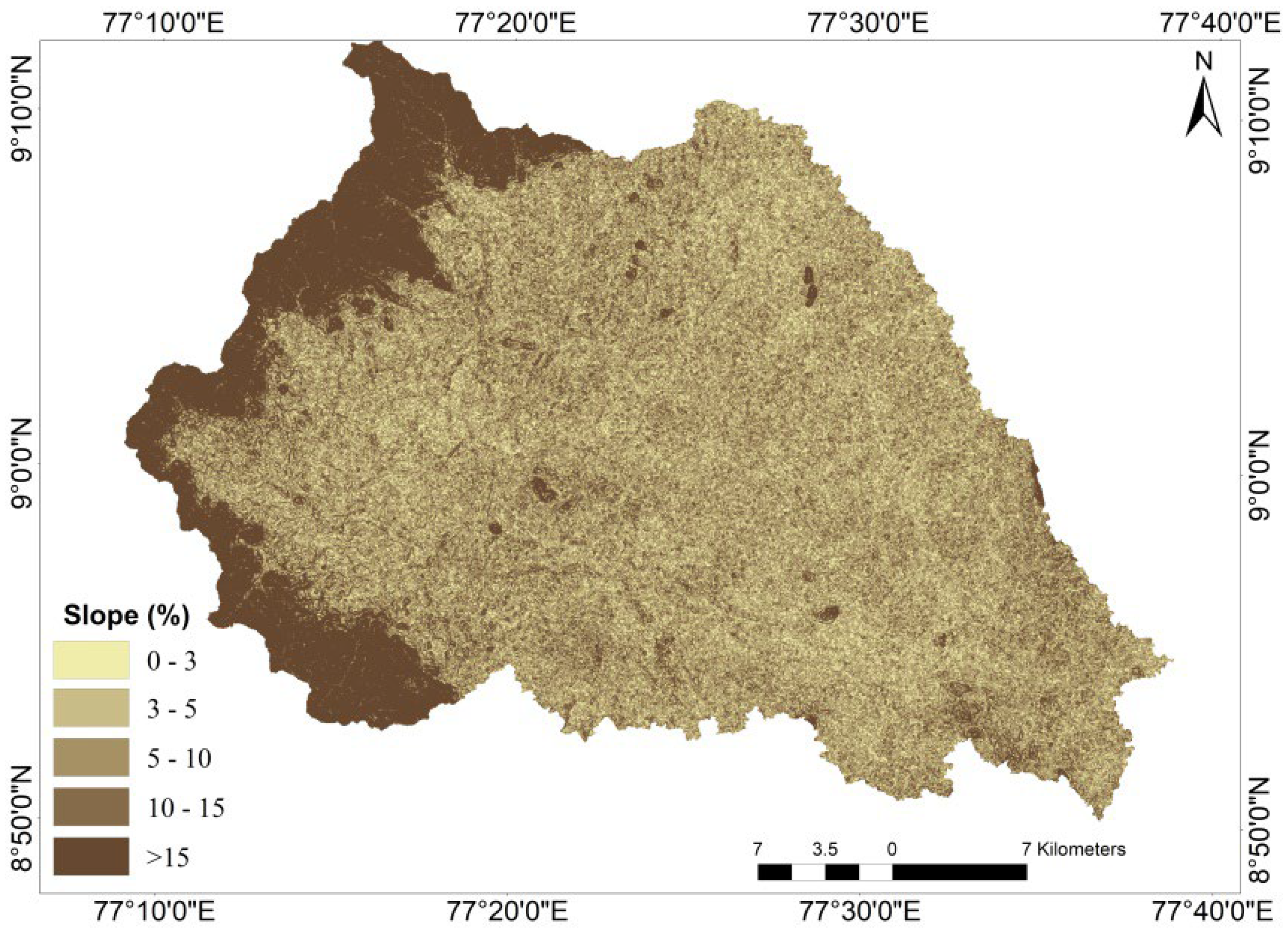
The HRU delineated for the combination of ten year interval LULC (i.e., 2001 and 2011), and time invariant soil and slope data in SWAT. These data were reclassified and overlay to construct the HRU geodatabase. HRU threshold definition was control the usage of combination data for this model development. The impact of HRU threshold on model performance was not yet systematically reported. Few researchers attempted with 0% or very low thresholds to preserve each unique landscape feature in the model development. However, most of the researchers agreed that 5% to 20% threshold was reasonably good [34]. In this study 5% threshold for soil and 10% threshold for LULC and slope were assigned.

2.3. Topography

The 30 m spatial resolution Aster-GDEM was used as topography map in this study. The Aster-GDEM was jointly developed and released by NASA of the United States and METI of Japan during 2011 [9]. The catchment boundary delineated in GIS platform by implement the deterministic-8 algorithm [35,36] over Aster GDEM. The outlets are further delineating into 11 sub catchments for the Chittar river basin (Figure 2). Aster-GDEM was also used to prepare the slope map over Chittar catchment as shown in Figure 3. The slope is quantifying the potential energy of the catchment by introducing the third dimension (i.e elevation) concept and so affecting the WBCs. The Integrated Mission for Sustainable Development (IMSD) classification was applied the five class of slope separated as show in Figure 3 [37]. The area cover with the very steep located at the upper most region (i.e., over Courtallam hills) of the catchment (Figure 3). Less than 3% of slope is largely contributed i.e flat plain that forms by erosion from the weathered particles. Because, land mass from the upper position of the western ghats drags into flat plain that causes the pediment formation.

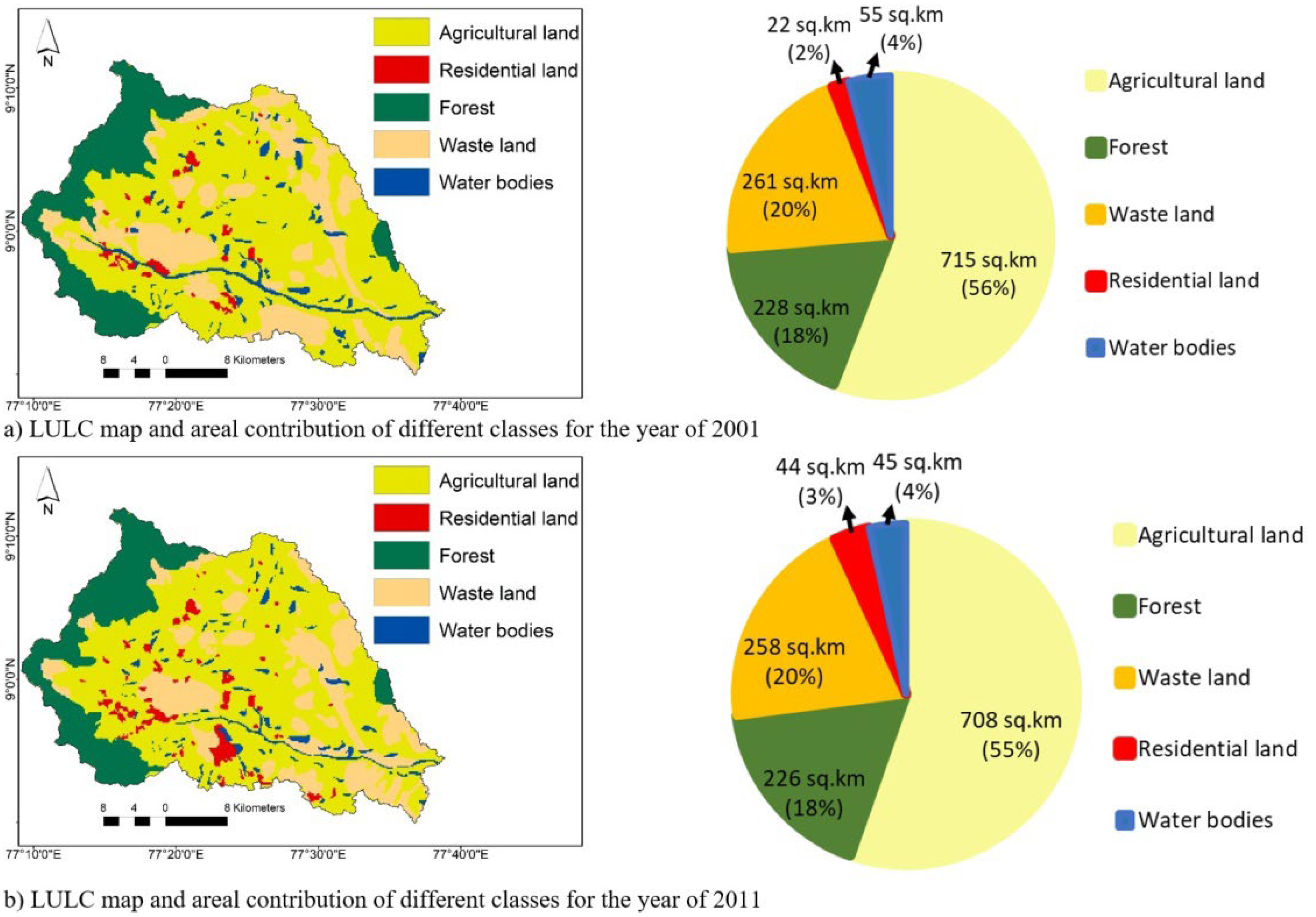
2.4. Land Use and Land Cover
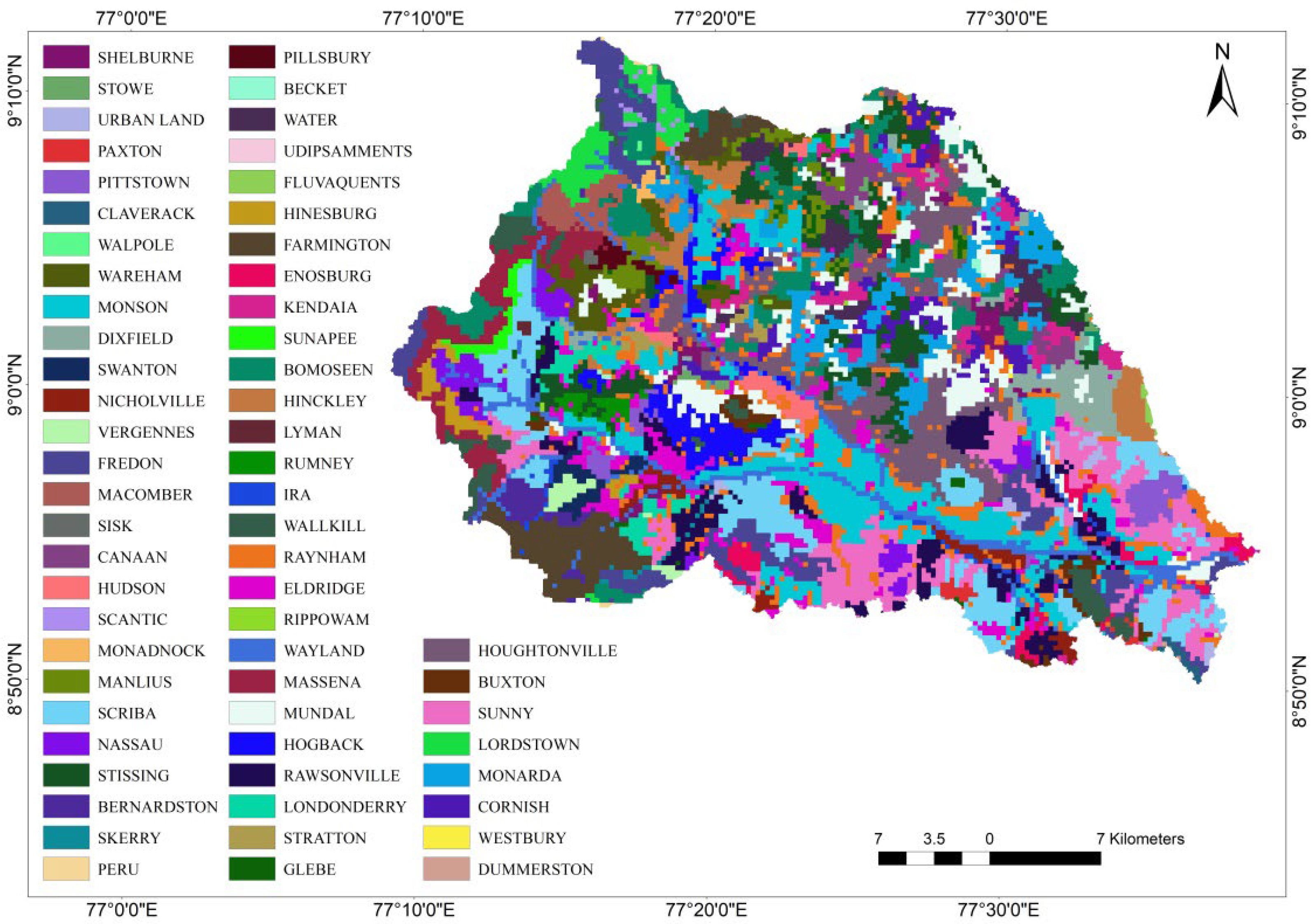
The LULC map delineated from Landsat imagery (URL: glovis.usgs.gov). Landsat is a multi-spectral image with 30 m of spatial resolution jointly released by NASA and USGS. The Visible and Near-Infrared (VNIR) region consists of blue (0.45–0.52 µm), green (0.52–0.60 µm) and red (0.63–0.69 µm) were captured using hyperspectral satellite sensors. Using the VNIR region of landsat imagery, LULC features were digitized in the GIS environment by mean of physical-interpretation [38]. The LULC was divided as per the Level 1 of NRSC Land Use and Land Cover Monitoring Division (2011–2012) guideline. NRSC LULC classification was proposing the residential land, agricultural land, forest, water bodies and waste land as first level of classification [26]. The areal change of LULC can be described in this catchment for the year 2001 and 2011. The processed LULC maps of Chittar catchment along with area in sq km and percentage contribution of each class were shown in Figure 4. LULC is part of the HRU which induces the finding the certain WBCs methods such as manning roughness coefficient and SCS-CN. By these parameters it evolves the WBCs such as runoff and infiltration. LULC also evolves the WBCs such as interception, depression storage and AE.
Mostly agricultural and forest land were jointly covered about 75% area in the catchment. Residential land (2%), water bodies (4%) and waste land (20%) contributed as shown in Figure 4. About 10 sq km of water bodies, 7 sq km of agricultural land, 2 sq km each waste land and forest land decreased during 2001 to 2011. Residential land was gained about 22 sq km during the same period. The mutual change of about 5–8% in agriculture and waste land was also observed. The agricultural to wasteland mutual conversion were mainly driven by the uneven distribution of monsoon rainfall. The conversion of waste to agricultural and residential land was more dominant for an increase in farming activities and urbanization driven by the population growth. The change in agricultural area poses a potential threat to sustainable development over catchment. The decrease in agriculture area reduces food production and rural employability. However increase in agricultural area brings addition stress to water and land resources. From the Figure 4, an area of residential land and water body gave the opposite in the area consumption. From 2001 to 2010, about 2 sq km of the forest is lost; thus, it leads to more runoff and soil erosion in the area. In the Chittar catchment, 20% of water bodies are decreased between the periods of 2001 to 2011. This change brings additional stress to ground water over the catchment. LULC has not shown much change for past years due to lack of smart cities development over it.

2.5. Soil Data

Soil is mainly contributed for their HRU delineation which is able to derive the hydrological soil groups based on soil properties. Infiltration, percolation, runoff and lateral flow has simulated from these soil properties. SWAT has several in build databases for soils, crops, fertilizers, slope and pesticides. In this study, the soil data was created by mapping block wise of soil data developed by Tamilnadu Agricultural University (TNAU), Coimbatore, Tamilnadu, India with SWAT in build soil database. The map was available in 1: 50,000 scale and having 75 classes over the Chittar catchment as shown in Figure 5. The soil classes cover more than 50 sq km over the catchment were Monson (95 sq km), Scriba (75 sq km), Houghtonville (75 sq km), Sunny (73 sq km), Raynham (66 sq km), Mundal (60 sq km), Bomoseen (58 sq km), Stissing (55 sq km), Fredon (51 sq km) and Monarda (50 sq km). The soil further regrouped in to four hydrological soil group based on soil texture, depth, sand, silt and clay content. In this Chittar catchment, almost 90% of soil cover was the part of the hydrological soil group C and D. First soil layer depth was about 300 mm and second layer was about 1000 mm. The soil was not varied with their time period and retains constant forever.

2.6. Meteorological Parameters

The meteorological station located over Cheranmadevi in the catchment data was used in this study. It is operated and maintain by the Government of Taminadu state on the state ground and surface water resources data centre, Chennai. Cheranmadevi observatory data contains the daily meteorology parameters like rainfall, relative humidity, wind speed, temperature etc. Meteorology parameters were used for estimating the energy distribution that affect the WBCs. The twenty-year (i.e., 2001–2020) daily meteorological data was used in this study. Over this twenty year period rainfall varied from 0 to 60 mm/day, temperature ranged from 16 to 43 °C, sunshine varied from 0 to 10.6 hrs, wind speed at 2 m height ranged from 0 to 11.6 kms/hr and finally relative humidity ranged from 22.5 to 93%. The solar radiation range cover in this catchment was about 3–12 kWh/m2/day. The north east monsoon contributed maximum rainfall over the Chittar catchment.

2.7. Model Calibration and Validation

In SWAT predefined program known as Calibration and Uncertainty Procedures (SWAT-CUP) is available freely for model calibration and validation. Many algorithms available in SWAT-CUP which includes SUFI-2 (Sequential Uncertainty FItting), PSO (Particle Swarm Optimization), MCMC (Markov Chain Monte Carlo), GLUE (Generalized Likelihood Uncertainty Estimation), and Parasol (Parameter Solution). In this study, SUFI-2 that enhanced the uncertainty analysis by their driving parameters of surface runoff component, so it was forced to calibrate the suitable parameters that processed in model calibration [39,40]. SUFI-2 fitted the model parameter values by performing sensitivity analysis. It identified sensitive of model parameters by knowing the significance level getting through objective function from the t-test. Thus, statistical output includes coefficient of determination (R2), Nash-Sutcliffe (NS), R-factor, P-factor, Percent BIAS (PBIAS), Root Mean Square Error (RMSE), Kling–Gupta efficiency etc. [31]. The P-factor and R-factor are measure the goodness of fit and uncertainty during calibration and validation. P-factor is the measure of percentage of observation within the given uncertainty bound. R-factor is providing average thickness for the given uncertainty band divided by the standard deviation of the measured data. Then, SWAT output variables were directly feed into the SWAT-CUP, performing the calibration, validation, uncertainty and sensitivity analysis [24]. The A.P Puram gauge discharge data for the period 2001–2015 was used for model calibration and validation. The monthly gauge discharge varied from 0 to 117 cumecs with standard deviation of 19 cumecs. The monthly average discharge is 10 cumecs. The model calibration was carried out in two phases such as pre-calibration (warm up) and post-calibration at monthly scale [25]. The pre-calibration period was from 2001 to 2003 (1–36 months); post-calibration is from 2004 to 2010 (37–120 months) and finally, validation is from 2011 to 2015 (121–180 months). The pre-calibration helped to identify the major sensitivity parameters and then further tuned in the post-calibration. Now days the GIS based time series of regional AE data is used in data scarce scenarios to calibrate and validate the hydrological model [33,41,42]. In this study, the performance of models was evaluated with an open source GIS based global AE model. Practitioners and researchers widely employ GLEAM (Global Land Evaporation Amsterdam Model) for arriving different components of evaporation [41]. As it is physical based global evaporation product which derived from multi-satellite observation and uses satellite based soil moisture as a constraint for computing potential evaporation [43]. It applies Priestley and Taylor equation to compute potential evaporation using remote sensing data. Computed potential evaporation from bare soil and canopy were converted in to AE using a multiplicative evaporative stress factor based on root-zone soil moisture and vegetation optical depth [41]. The dataset provides monthly and daily scale AE over 0.25° grid resolution (i.e., 27 km by 27 km grid) from 1980 to 2021. Khan et al. [44] reported that GLEAM provides relatively minimum error and uncertainties over global evaporation product such as Global Land Data Assimilation System (GLDAS) and MOD16. The selection of this data was based on its satisfactory performance in the previous studies [41,43,44,45]. The monthly gridded AE data over few sub catchments were downloaded for this purpose.

3. Results and Discussions

The slope, soil, ten year interval LULC (i.e., 2001 and 2011), daily meteorological parameters during 2001–2020 and gauge discharge data were used for model development. The Chittar catchment delineated from the Thamirabarani basin for the river gauge discharge point (outlet) which is located at A.P Puram (Figure 2). Chittar catchment subdivides into the 11 sub catchments as shown in Figure 6. The assigned Sub Catchment (SC) number along with its area in sq km and perimeter in km were also provided in the Figure 6. The sub catchments were varied in their size and shape because it delineates from the undulating topography i.e DEM. Middle part of catchments has smaller sub catchments; because main branch of Chittar river that flowing in the landscape without connection of tributary. Rests of larger sub catchments were major tributaries sub catchments.

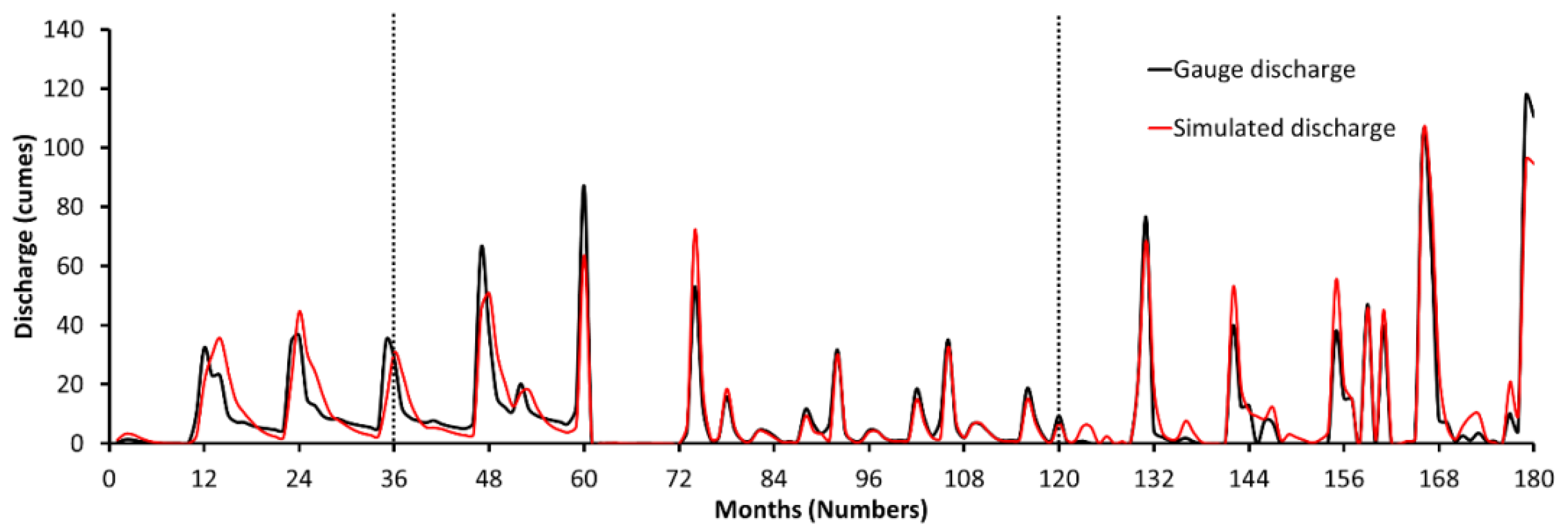
3.1. Calibration and Validation

The SWAT-CUP implemented SUFI-2 adoptable for model calibration and validation using the gauge discharges [25]. The global and local sensitivity analyses were the widely applied techniques. The global sensitivity analysis attempts to access simultaneously changes in two or more parameters using multiple regression analysis. Local sensitivity analysis attempts to measures effect of parameter one by one through linear regression analysis. The two approaches having their own advantages and challenges [20,22]. In this study Global sensitivity analysis was performed to identify the relative sensitivity of model parameter at catchment scale [46]. The relative sensitivity of model parameter was catchment specify. It also depends on model structure, state variables and spatiotemporal resolution of input parameter. The sensitivity analysis results were used in parameter optimization during calibration process by forcing local conditions. This will reduce prediction uncertainty and computational effort. Further it assists in analyzing interaction among parameters and its range and spatial variability which in turn influence the model performance. Among the 43 model parameters incorporated in the model development, over Chittar catchment 18 were most sensitive to five WBCs. The value of 18 calibrated model parameters were shown in Table 1. The major contribution of each model parameters on the hydrological process was also provided in Table 1 for better understanding. Table 1 show the relative rank order of model parameters which was assigned based on student t distribution and p-value [31]. The model parameter with largest student t distribution (i.e., most sensitive) along with lowest p value (i.e., most significant) was assigned with rank 1 as shown in Table 1. The model parameters CN2, GW_DELAY, ALPHA_BNK and SOL_AWC were relatively more significant model parameters (p value < 0.01) at catchment scale. The model parameter t stat were varied from −5.96 to 5.33. Outcome of study identified that CN2 as most sensitive among the 18 model parameters. The CN2 values varied −0.2 (high infiltration) to +0.2 (high runoff). About 90% catchment area was covered soil with low to medium infiltration (i.e., hydrological soil group C and D). Accordingly CN2 calibrated value was closer 0. The next sensitive parameters were Groundwater delay time (GW_DELAY) and Base flow alpha factor for bank storage (ALPHA_BNK). The GW_DELAY controls the lag time in water leaving from soil layer to shallow aquifer. A larger GW_DELAY will enable more abstractions from the unsaturated zone and vice versa. The ALPHA_BNK characterizes the bank storage recession to main channel. It varies 1 denoting flat recessions to near zero for steep recessions.
The model validation was carried out using unseen gauge discharge data. The 95 percent prediction uncertainty (95PPU) was helpful to predict from the model performance. The SWAT simulated monthly discharge were plotted in the Figure 7 shows a reasonably fit with observed discharge. The simulated discharge was not perfectly matching with observed discharge during pre-calibration period and reasonably fitting well during post-calibration and validation periods. The model not was able to predict accurately few observed peaks during calibration and validation periods. This may be due to the presence of few small dry tanks over the Chittar catchment; which was not included in the model development.
The pre-calibration outputs gave the result of R2 and NS both equal to 0.75. Again, calibration outputs gave the result as R2 was 0.94 and NS was 0.89. The validation period gave the R2 was 0.81 and NS was 0.76. The PBIAS was ranged between the −1.7 to 2.7 and the baseline has not deviated more the ±3. Similarly, RMSE was half stabilized at 0.5 mm. The detail statistical performance indexes were given in the Table 2. As well as R-factor was reduced in to small values at calibration and validation period but P-factor is raised in the calibration and again reduced in validation. The small values in R-factor and large values in P-factor was acceptable at 95 PPU [23]. Thus, PBIAS lies within 3%, R2 and NS lies above 0.7 were supports the reasonable fit of model simulation with observed discharge [46].
The GLEAM provides 0.25° grid resolution monthly and daily AE data in mm from 1980 to 2021 at global scale. The coarse spatial resolution of the data hinders its application to catchment scale studies. However, many researchers were incorporated GLEAM data to calibrate and validate the catchment scale hydrological models [33,41,42,43]. In this study GLEAM v3.6a monthly AE data from 2001 to 2020 (i.e., 240 months) were used to validate sub catchment scale SWAT simulated AE. For this time series of monthly gridded AE data over the sub catchments SC6, SC10 and SC11 were extracted from the global GLEAM data. The geo coordinate of the grid cell data used in this study were (77.375° E: 8.875° N), (77.375° E: 9.125° N) and (77.625° E: 8.875° N) for the sub catchments SC6, SC10 and SC11 respectively. The linear correlation plot of SWAT and GLEAM modeled monthly AE at over the sub catchments SC6, S10 and S11 were shown in Figure 8. The estimated R2 during this comparison were 0.83, 0.76 and 0.84 respectively for sub catchments SC6, S10 and SC11. The RMSE for the sub catchments SC6, S10 and SC11 were 10 mm, 9 mm and 15 mm respectively. The correlation plot average gradient was about 0.9 over three sub catchments by forcing intercept to zero. This supports that SWAT and GLEAM modeled monthly AE were reasonably matching well over the three sub catchments. The AE were generally well distributed around the straight line and shows a strong positive correlation. The consistency of model performance over sub catchments confirmed the reliability and versatility of the model over the Chittar catchment. The high RMSE reveals that a significant difference exists at individual values. This mismatch at individual values was very common while regional model compared over local studies.

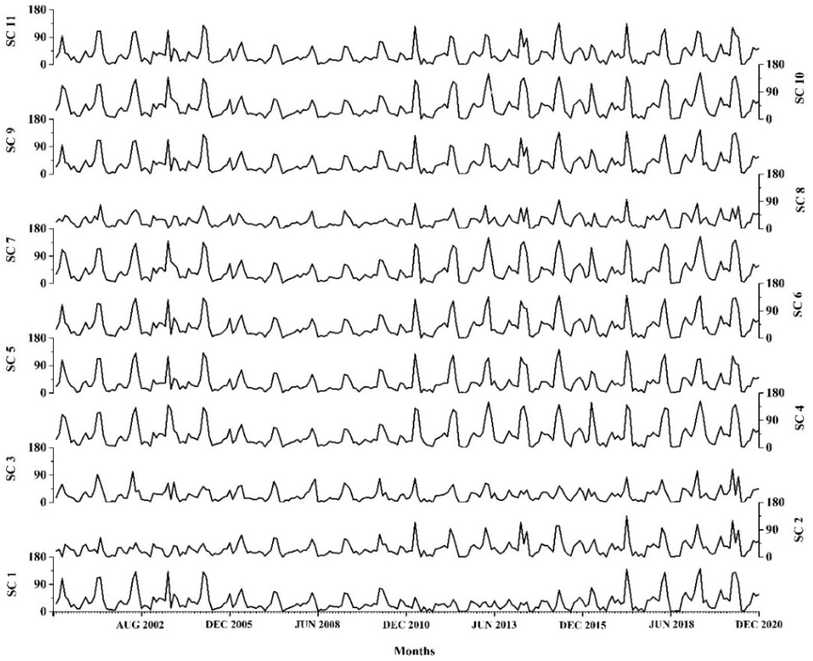
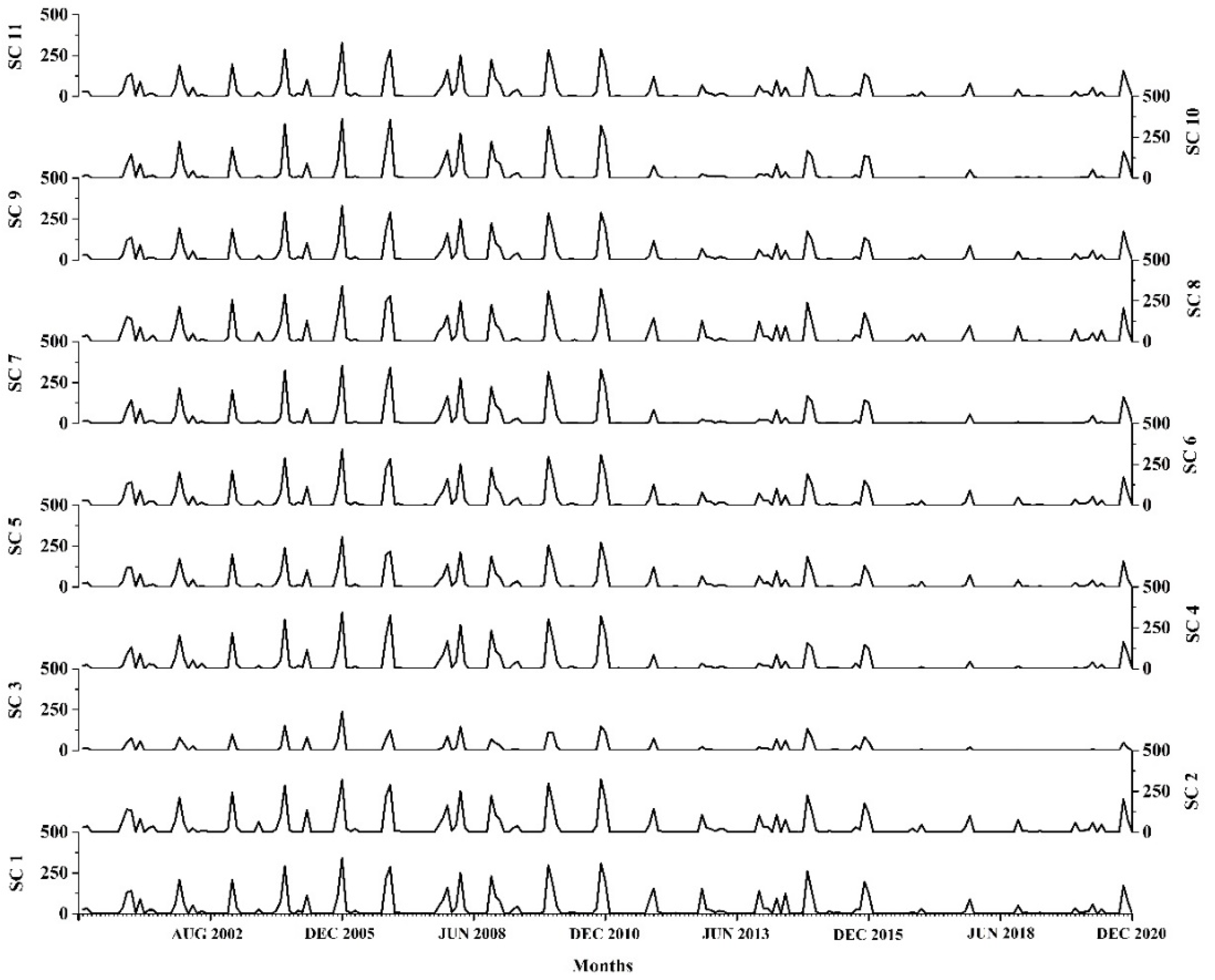
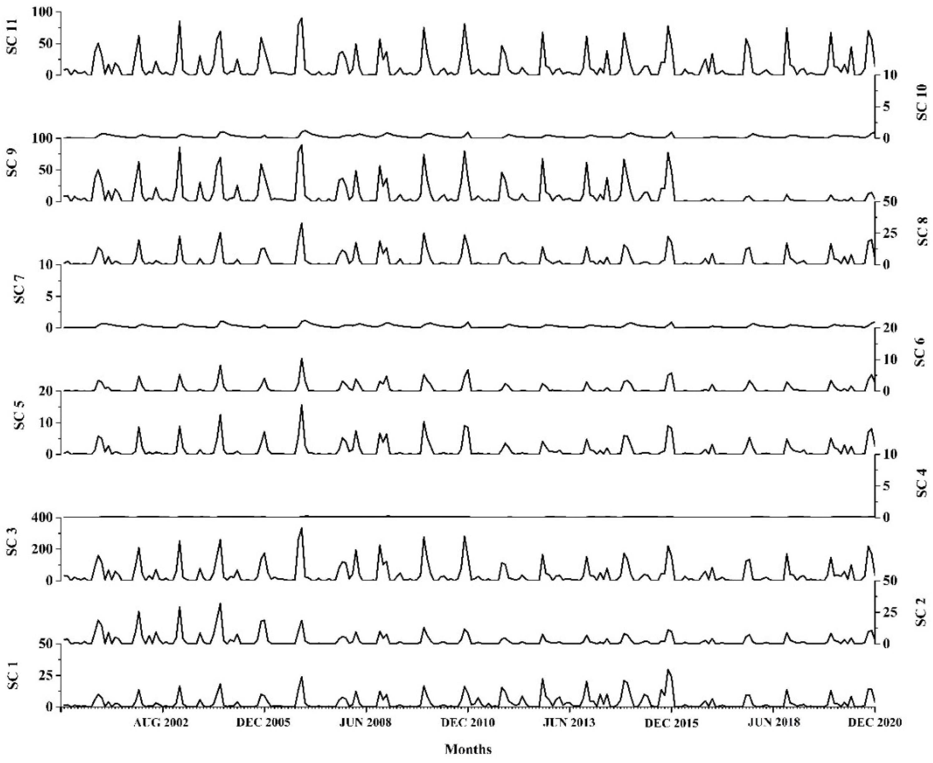
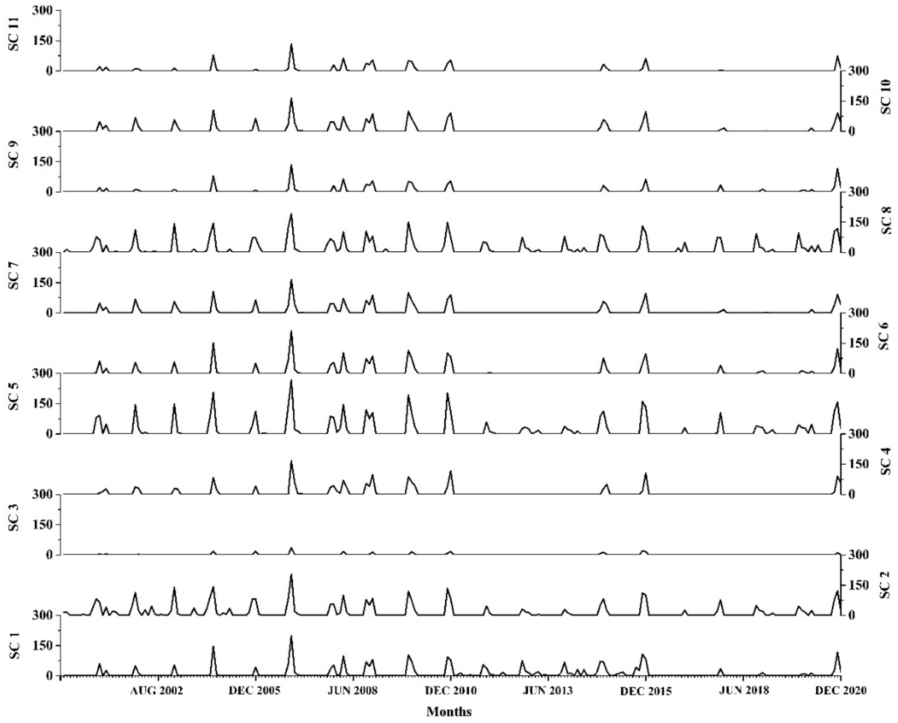
3.2. Water Balance Components

In the tropical climate in south India, it behaves the seasonal variation in the temperature as well as rainfall that reflected in the WBCs anomaly. Catchment spans the latitude of 8°45′ N to 9°15′N lies in tropical zone, so it is semi-arid climate that have hot summers and warm to cool winters. In the Chittar catchment, hot weather (maximum temperature) happened for about seven months in an annum. So, it causes the more ET in the agricultural and forest land (i.e., 75% area); also converts the surface water bodies to dry land. The SWAT model delineated the HRU as per the given soil, slope, ten year interval LULC and simulated WBCs by forcing the daily meteorological variables for the period 2001–2020. The output shows monthly WBCs such as AE, surface runoff, lateral flow, percolation, and SW at catchment and sub catchment level in mm. The SWAT is a lumped model at HRU and at the same time shows the spatial variability at sub-catchment level. Accordingly Figure 9, Figure 10, Figure 11, Figure 12 and Figure 13 provided here to show the spatial variability of five WBCs at 11 sub-catchments. The monthly scale of WBCs at every sub catchment in mm from January 2001 to December 2020 was shown in Figure 9, Figure 10, Figure 11, Figure 12 and Figure 13. Many previous studies reporting that complexity in catchment scale WBCs that mask impact of LULC, meteorological, and hydrological processes associated with local conditions [6]. The prediction of sub-catchment or further small scale variability of WBCs is important for easy and accurate decision making. The assigned SC number was shown in Figure 6. During 2016–2018 all five WBCs were relatively very low throughout the catchment. This may be due to severe drought over south India because of failure of northeast monsoon. The Figure 9 shows that monthly AE values of 11 sub catchment. The reported sub catchment level monthly maximum WBCs were 526 mm of rainfall, 324 mm of surface runoff, 123 mm of AE, 159 mm of percolation, 64 mm of lateral flow and 193 mm of SW. It was observed maximum rainfall that received during September to December due to onset of northeast monsoon. Out the considered 20 years period the minimum rainfall was reported in year 2008 over the catchment. The monsoon rainfall is the major source for SW in the catchment. The SW shows the trend with respect to gain and loss components in the catchment. Moreover, surface runoff, lateral flow and percolation are the components cause the losses and also making the similar effect of oscillations with respect to rainfall. The AE was reversed trend with other WBCs; it appears to be maximum from January to August. So, it seems to be loss of water in the catchment over the period, which happened due to evaporation from SW, and other components likely lateral flow and percolation put into the subsurface by the gravity action. The sub catchment of monthly mean AE varies from 25 mm to 43 mm with standard deviation varies 20 mm to 38 mm. All the 11 sub catchments AE reached simultaneously maximum during April/May at every year. The monthly AE was not showing much variation during 2005 to 2011. This may due to unusual warming reported over south India due to enhanced convection in southern Indian Ocean and forced anticyclonic activities over the Bay of Bengal [47]. The AE peaks were generally high during 2016–2018 at all sub catchment. These AE peaks occurs due to failure of north east monsoon over the south India during 2016–2018 [48]. The SC8 reported minimum AE value throughout the simulation period. This may be due to combined effect high slope along with low permeable soil layer that will decrease the SW and subsequently reduces the AE over the SC8.
The surface runoff shows similar trend at all sub catchments (Figure 10). South India was hit by 150 years severe drought during 2016–2018 due to failure of northeast monsoon [48]. This brings down the surface runoff at all sub catchments after 2013. The monthly sub catchment level surface runoff varied from 0 to 360 mm with standard deviation varies 32 mm to 67 mm. The minimum and maximum annual average surface runoffs were 150 mm at SC3 and 387 mm at SC8. The steep slope and largest forest cover over the SC3 increase lateral flow that brings down the surface runoff. The increased anthropogenic activities and high drainage density over SC8 increase the surface runoff (Figure 4). The increased surface runoff brings soil erosion and flooding over catchment. Generally, lateral flow was not showing much variation over Chittar catchment as shown in Figure 11. The surface runoff and lateral flow are sharing the rain water on the land surface after meeting other abstraction. As the increases lateral flow considerable decreases in the surface runoff. However, both have strong positive correlated with rainfall. The standard deviation of monthly lateral flow varies from 0 to 63 mm. The sub catchment lateral flow and surface runoff reached peaks simultaneously during monsoon period. The monthly average lateral flow of three sub catchments (viz. SC3, SC9 and SC11) were more than 10 mm. The maximum monthly lateral flow was reported in SC3 during November 2006 with value equal to 333 mm. The lateral flow increases the SW only for a short period and further contributing in to runoff component [49]. The mountainous forested environment in SC3 increases the lateral flow that subsequently reduces surface runoff, AE and SW.
The monthly trend of sub catchment scale percolation was shown in Figure 12. The spatiotemporal distributions of percolation are influencing the ground water recharge, leaching and SW availability. The percolation mainly depends on the soil characteristics, LULC and slope. The average sub catchment percolation was varying from 1 mm to 18 mm with standard deviation ranging from 4 to 44 mm. The maximum percolation was observed during October/November every year due to onset of north east monsoon. Over all the maximum percolation reported at November 2006 for all sub catchment. This may be due to continuous heavy rainfall occurs over south Tamilnadu [50] during November, 2006. This heavy rainfall induces huge flood and large number landslides over south western ghats mountain [50]. The percolation in SC3 was observed to be low throughout the simulation period (Figure 12). The most part of the SC3 lies over the western ghats mountain region. Accordingly, the low permeable hard rock formation over the SC3 limits the percolation. The percolation at all sub catchments was low during 2016–2018 due to failure of northeast monsoon [20]. Figure 13 shows the variations of monthly sub catchment level in SW during 2001–2020. The SW is an important parameter that controlling exchange of heat energy and water between land and atmosphere. As a result, SW play a key role in crop water requirement, crop selection, crop yield, soil erosion, leaching, slope stability, flood and drought management, weather patterns etc. The monthly sub catchment level SW varied from 0 to 426 mm with standard deviation 20 to 120 mm. The monthly average SW of SC1, SC2, SC3 and SC8 were below 50 mm; it may consider as drought prone area within this catchment. The constructions of rain water harvesting and artificial ground water recharge infrastructure over these sub catchments were important for sustainable agricultural activity. The overall low and high SW was observed in SC8 and SC4 respectively throughout the simulation period. The high percolation in SC8 remove most of the water from root zone consequently reduces the SW. Similarly, low percolation in SC4 allows more SW in root zone. It was observed that SW suddenly increases at all sub catchments on set of north east monsoon (September/October). After the monsoon period, decline trend were observed due to removal of SW by ET and percolation. The SW was also affected by the soil characteristics, LULC and slope of the area. Generally, observed that at all sub catchments of SW were more than 50 mm from September to March.

4. Conclusions

This study demonstrates that, SWAT is used as a tool to delineate the spatiotemporal distribution of WBCs over a catchment under limited data scenario. The model can predict WBCs such as, AE, surface runoff, lateral flow, percolation and SW by forcing the meteorological, LULC, topography and soil data. The model invokes time invariant soil and topography data along with ten year interval LULC and daily meteorological data. The model was calibrated with measured gauge discharge using SUFI-2 algorithm available in SWAT-CUP. During validation the R2 and NS were 0.81 and 0.76 respectively. Further the monthly AE from 2001–2020 was reasonably matching with GIS based GLEAM evaporation extracted at sub catchments. Statistical indexes support the perfection of model development and it is most efficient and more significance for the water balance modeling over the Chittar catchment. The recent LULC of 2001 and 2011 were prepared and analyzed the LULC changes. The daily meteorological variables of Cheranmadevi station for period 2001 to 2020 were used for the model development. The outcome of the study provides monthly WBCs trends such as AE, surface runoff, lateral flow, percolation, and SW at 11 sub catchments. Major conclusions drawn from the study were as follow:
  • The residential land area doubled between 2001 and 2011, indicating frenzied construction activity over the catchment. The annual average reduction of water bodies over the catchment is about 1 sq. km/year. The increase in residential land and mutual changes among the other classes leads to an increase in surface runoff and reduction in lateral flow and percolation.
  • Out of the four simulated WBCs, surface runoff and AE show maximum variations at monthly scale at all sub catchment. The lateral flow and percolation shown least variation. Developing appropriate rain water harvesting and artificial groundwater recharge infrastructures helps to reduce flood, soil erosion and drought over catchment.
  • Relative sensitivity analysis depicted that CN2 gives highly sensitive parameter followed by GW_DELAY and ALPHA_BNK over the catchment.
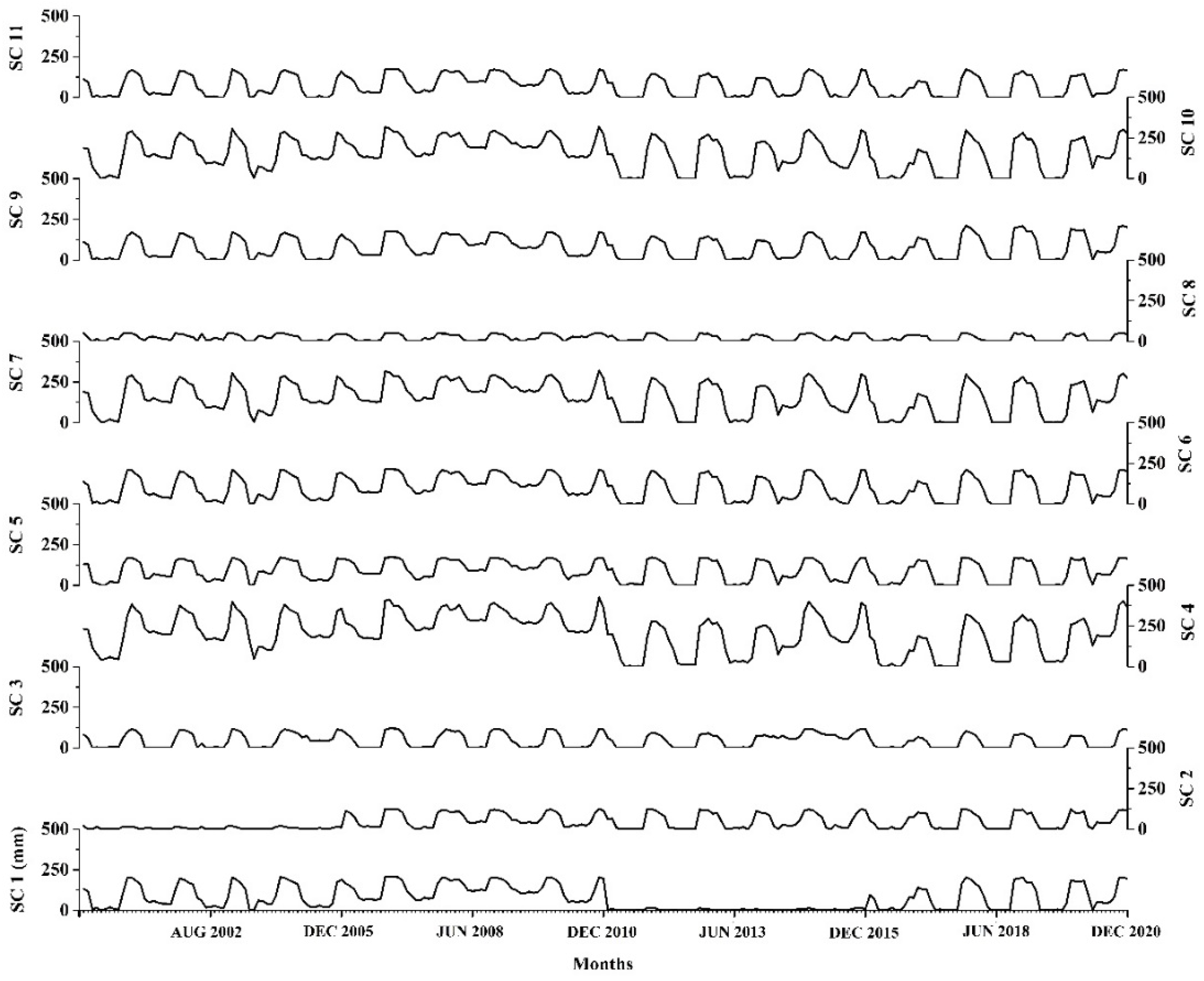
  • Generally, SW was more than 50 mm (i.e., above 12% SW) from October to March at all sub catchment. Hence the famers over the Chittar catchment may prefer to raise single crop.
  • The SW in the upstream sub catchments SC2, SC3 and SC8 were low throughout the simulation period. This may contribute to increase the frequency and intensity of agricultural drought over the sub catchment.
  • The average monthly percolation of SC1, SC2, SC5 and SC8 were more than 10 mm. The higher percolation increases natural groundwater recharge and leaching in soil.
  • The mountains forested environment in SC3 increases the lateral flow that subsequently reduces surface runoff, ET and SW. The high lateral flow enhance transport soil and its nutrient in to water bodies.
The mapping WBCs is helped to avoid the scarcity of water resources and retain the sustainability at catchment scale. It is one of the critical inputs for practitioner, policy maker’s researchers and NGO to develop and install more efficient integrated water resources management and command area development programs. Further, it is useful for selecting and design the water harvesting technique such as canal irrigation, check dams, dam and reservoir operation, percolation tanks and pits etc.

Author Contributions

D.P. wrote the initial draught of the research article and completed the modelling portion. S.K. conceptualized the work, conducted the literature search, and revised the manuscript. Also, S.K. offered technical comment on the draught report as well as useful suggestions to make the manuscript better. M.K. oversaw and made recommendations for the manuscript’s modification. All authors have read and agreed to the published version of the manuscript.

Funding

This research received no external funding. The APC was funded by Vellore Institute of Technology, Chennai, India.

Data Availability Statement

The corresponding author will provide the datasets used and/or analysed in the work upon reasonable request.

Acknowledgments

The Vellore Institute of Technology in Chennai graciously provided a workstation and other amenities for the authors to conduct their research. Additionally, the authors thank the state ground and surface water resources data centre, Government of Tamilnadu, India, and India-Water Resource Information System (India-WRIS) for supplying the study’s essential data. The Landsat series images was provided by USGS Earth Explorer, which the authors gratefully acknowledge. Authors thank anonymous reviewers for their constructive comments as well as suggestions, which are very helpful for improving the quality of the manuscript.

Conflicts of Interest

The authors declare no conflict of interest.

References

  1. Mishra, A.K.; Singh, V.P. A Review of Drought Concepts. J. Hydrol. 2010, 391, 202–216. [Google Scholar] [CrossRef]
  2. Llasat, M.C.; Llasat-Botija, M.; Barnolas, M.; Ĺopez, L.; Altava-Ortiz, V. An Analysis of the Evolution of Hydrometeorological Extremes in Newspapers: The Case of Catalonia, 1982–2006. Nat. Hazards Earth Syst. Sci. 2009, 9, 1201–1212. [Google Scholar] [CrossRef] [Green Version]
  3. Oeurng, C.; Sauvage, S.; Sánchez-Pérez, J.M. Assessment of Hydrology, Sediment and Particulate Organic Carbon Yield in a Large Agricultural Catchment Using the SWAT Model. J. Hydrol. 2011, 401, 145–153. [Google Scholar] [CrossRef] [Green Version]
  4. Dickinson, R.E. Land Processes in Climate Models. Remote Sens. Environ. 1995, 51, 27–38. [Google Scholar] [CrossRef]
  5. Liang, X.; Xie, Z. Important Factors in Land-Atmosphere Interactions: Surface Runoff Generations and Interactions between Surface and Groundwater. Glob. Planet. Change 2003, 38, 101–114. [Google Scholar] [CrossRef]
  6. Strasser, U.; Mauser, W. Modelling the Spatial and Temporal Variations of the Water Balance for the Weser Catchment 1965–1994. J. Hydrol. 2001, 254, 199–214. [Google Scholar] [CrossRef]
  7. Yang, D.; Sun, F.; Liu, Z.; Cong, Z.; Ni, G.; Lei, Z. Analyzing Spatial and Temporal Variability of Annual Water-Energy Balance in Nonhumid Regions of China Using the Budyko Hypothesis. Water Resour. Res. 2007, 43, W04426. [Google Scholar] [CrossRef]
  8. Chang, H.; Jung, I.W. Spatial and Temporal Changes in Runoff Caused by Climate Change in a Complex Large River Basin in Oregon. J. Hydrol. 2010, 388, 186–207. [Google Scholar] [CrossRef]
  9. Kundu, S.; Khare, D.; Mondal, A. Past, Present and Future Land Use Changes and Their Impact on Water Balance. J. Environ. Manag. 2017, 197, 582–596. [Google Scholar] [CrossRef]
  10. Graf, R.; Jawgiel, K. The Impact of the Parameterisation of Physiographic Features of Urbanised Catchment Areas on the Spatial Distribution of Components of the Water Balance Using the WetSpass Model. ISPRS Int. J. Geo-Inf. 2018, 7, 278. [Google Scholar] [CrossRef]
  11. Amin, A.; Iqbal, J.; Asghar, A.; Ribbe, L. Analysis of Current and Futurewater Demands in the Upper Indus Basin under IPCC Climate and Socio-Economic Scenarios Using a Hydro-Economic WEAP Model. Water 2018, 10, 537. [Google Scholar] [CrossRef] [Green Version]
  12. Li, S.; Yang, H.; Lacayo, M.; Liu, J.; Lei, G. Impacts of Land-Use and Land-Cover Changes on Water Yield: A Case Study in Jing-Jin-Ji, China. Sustainability 2018, 10, 960. [Google Scholar] [CrossRef] [Green Version]
  13. Garg, V.; Aggarwal, S.P.; Gupta, P.K.; Nikam, B.R.; Thakur, P.K.; Srivastav, S.K.; Senthil Kumar, A. Assessment of Land Use Land Cover Change Impact on Hydrological Regime of a Basin. Environ. Earth Sci. 2017, 76, 635. [Google Scholar] [CrossRef]
  14. Xu, C.Y.; Singh, V.P. A Review on Monthly Water Balance Models for Water Resources Investigations. Water Resour. Manag. 1998, 12, 20–50. [Google Scholar] [CrossRef]
  15. Hurkmans, R.T.W.L.; De Moel, H.; Aerts, J.C.J.H.; Troch, P.A. Water Balance versus Land Surface Model in the Simulation of Rhine River Discharges. Water Resour. Res. 2008, 44, W01418. [Google Scholar] [CrossRef] [Green Version]
  16. Wang, Q.J.; Pagano, T.C.; Zhou, S.L.; Hapuarachchi, H.A.P.; Zhang, L.; Robertson, D.E. Monthly versus Daily Water Balance Models in Simulating Monthly Runoff. J. Hydrol. 2011, 404, 166–175. [Google Scholar] [CrossRef]
  17. Boughton, W. The Australian Water Balance Model. Environ. Model. Softw. 2004, 19, 943–956. [Google Scholar] [CrossRef]
  18. White, E.D.; Easton, Z.M.; Fuka, D.R.; Collick, A.S.; Adgo, E.; McCartney, M.; Awulachew, S.B.; Selassie, Y.G.; Steenhuis, T.S. Development and Application of a Physically Based Landscape Water Balance in the SWAT Model. Hydrol. Processes 2011, 25, 915–925. [Google Scholar] [CrossRef]
  19. Patil, A.; Ramsankaran, R.A.A.J. Improving Streamflow Simulations and Forecasting Performance of SWAT Model by Assimilating Remotely Sensed Soil Moisture Observations. J. Hydrol. 2017, 555, 683–696. [Google Scholar] [CrossRef]
  20. Swain, J.B.; Patra, K.C. Impact Assessment of Land Use/Land Cover and Climate Change on Streamflow Regionalization in an Ungauged Catchment. J. Water Clim. Change 2019, 10, 554–568. [Google Scholar] [CrossRef]
  21. Loliyana, V.D.; Patel, P.L. A Physics Based Distributed Integrated Hydrological Model in Prediction of Water Balance of a Semi-Arid Catchment in India. Environ. Model. Softw. 2020, 127, 104677. [Google Scholar] [CrossRef]
  22. Cibin, R.; Sudheer, K.P.; Chaubey, I. Sensitivity and Identifiability of Stream Flow Generation Parameters of the SWAT Model. Hydrol. Processes 2010, 24, 1133–1148. [Google Scholar] [CrossRef]
  23. Poméon, T.; Diekkrüger, B.; Springer, A.; Kusche, J.; Eicker, A. Multi-Objective Validation of SWAT for Sparsely-GaugedWest African River Basins—A Remote Sensing Approach. Water 2018, 10, 451. [Google Scholar] [CrossRef] [Green Version]
  24. Abbaspour, K.C.; Rouholahnejad, E.; Vaghefi, S.; Srinivasan, R.; Yang, H.; Kløve, B. A Continental-Scale Hydrology and Water Quality Model for Europe: Calibration and Uncertainty of a High-Resolution Large-Scale SWAT Model. J. Hydrol. 2015, 524, 733–752. [Google Scholar] [CrossRef] [Green Version]
  25. Lu, Z.; Zou, S.; Xiao, H.; Zheng, C.; Yin, Z.; Wang, W. Comprehensive Hydrologic Calibration of SWAT and Water Balance Analysis in Mountainous Watersheds in Northwest China. Phys. Chem. Earth 2015, 79–82, 76–85. [Google Scholar] [CrossRef]
  26. Allen, R.G.; Pruitt, W.O.; Wright, J.L.; Howell, T.A.; Ventura, F.; Snyder, R.; Itenfisu, D.; Steduto, P.; Berengena, J.; Yrisarry, J.B.; et al. A Recommendation on Standardized Surface Resistance for Hourly Calculation of Reference ETo by the FAO56 Penman-Monteith Method. Agric. Water Manag. 2006, 81, 1–22. [Google Scholar] [CrossRef]
  27. Rostamian, R.; Jaleh, A.; Afyuni, M.; Mousavi, S.F.; Heidarpour, M.; Jalalian, A.; Abbaspour, K.C. Application of a SWAT Model for Estimating Runoff and Sediment in Two Mountainous Basins in Central Iran. Hydrol. Sci. J. 2008, 53, 977–988. [Google Scholar] [CrossRef]
  28. Sloan, P.G.; Moore, I.D. Modeling Subsurface Stormflow on Steeply Sloping Forested Watersheds. Water Resour. Res. 1984, 20, 1815–1822. [Google Scholar] [CrossRef] [Green Version]
  29. Neitsch, S.L.; Arnold, J.G.; Kiniry, J.R.; Williams, J.R. Soil & Water Assessment Tool Theoretical Documentation Version 2009; Texas Water Resources Institute: College Station, TX, USA, 2011; pp. 1–647. [Google Scholar]
  30. Ritchie, J.T. Model for Predicting Evaporation from a Row Crop with Incomplete Cover. Water Resour. Res. 1972, 8, 1204–1213. [Google Scholar] [CrossRef] [Green Version]
  31. Zare, M.; Azam, S.; Sauchyn, D. Evaluation of Soil Water Content Using SWAT for Southern Saskatchewan, Canada. Water 2022, 14, 249. [Google Scholar] [CrossRef]
  32. Abbaspour, K.C.; Yang, J.; Maximov, I.; Siber, R.; Bogner, K.; Mieleitner, J.; Zobrist, J.; Srinivasan, R. Modelling Hydrology and Water Quality in the Pre-Alpine/Alpine Thur Watershed Using SWAT. J. Hydrol. 2007, 333, 413–430. [Google Scholar] [CrossRef]
  33. Nesru, M.; Shetty, A.; Nagaraj, M.K. Multi-Variable Calibration of Hydrological Model in the Upper Omo-Gibe Basin, Ethiopia. Acta Geophys. 2020, 68, 537–551. [Google Scholar] [CrossRef]
  34. Her, Y.; Frankenberger, J.; Chaubey, I.; Srinivasan, R. Threshold Effects in HRU Definition of the Soil and Water Assessment Tool. Trans. ASABE 2015, 58, 367–378. [Google Scholar] [CrossRef]
  35. Lin, W.T.; Chou, W.C.; Lin, C.Y.; Huang, P.H.; Tsai, J.S. WinBasin: Using Improved Algorithms and the GIS Technique for Automated Watershed Modelling Analysis from Digital Elevation Models. Int. J. Geogr. Inf. Sci. 2008, 22, 47–69. [Google Scholar] [CrossRef]
  36. Yang, W.; Hou, K.; Yu, F.; Liu, Z.; Sun, T. A Novel Algorithm with Heuristic Information for Extracting Drainage Networks from Raster DEMs. Hydrol. Earth Syst. Sci. Discuss. 2010, 7, 441–459. [Google Scholar]
  37. Pandi, D.; Kothandaraman, S.; Kuppusamy, M. Delineation of Potential Groundwater Zones Based on Multicriteria Decision Making Technique. J. Groundw. Sci. Eng. 2020, 8, 180–194. [Google Scholar]
  38. Areendran, G.; Rao, P.; Raj, K.; Mazumdar, S.; Puri, K. Land Use/Land Cover Change Dynamics Analysis in Mining Areas of Singrauli District in Madhya Pradesh, India. Trop. Ecol. 2013, 54, 239–250. [Google Scholar]
  39. Van Griensven, A.; Bauwens, W. Multiobjective Autocalibration for Semidistributed Water Quality Models. Water Resour. Res. 2003, 39, 1348. [Google Scholar] [CrossRef]
  40. van Griensven, A.; Meixner, T.; Grunwald, S.; Bishop, T.; Diluzio, M.; Srinivasan, R. A Global Sensitivity Analysis Tool for the Parameters of Multi-Variable Catchment Models. J. Hydrol. 2006, 324, 10–23. [Google Scholar] [CrossRef]
  41. Martens, B.; Miralles, D.G.; Lievens, H.; van der Schalie, R.; de Jeu, R.A.M.; Fernández-Prieto, D.; Beck, H.E.; Dorigo, W.A.; Verhoest, N.E.C. GLEAM v3: Satellite-Based Land Evaporation and Root-Zone Soil Moisture. Geosci. Model Dev. 2017, 10, 1903–1925. [Google Scholar] [CrossRef] [Green Version]
  42. Odusanya, A.E.; Schulz, K.; Biao, E.I.; Degan, B.A.S.; Mehdi-Schulz, B. Evaluating the Performance of Streamflow Simulated by an Eco-Hydrological Model Calibrated and Validated with Global Land Surface Actual Evapotranspiration from Remote Sensing at a Catchment Scale in West Africa. J. Hydrol. Reg. Stud. 2021, 37, 100893. [Google Scholar] [CrossRef]
  43. Yang, X.; Yong, B.; Ren, L.; Zhang, Y.; Long, D. Multi-Scale Validation of GLEAM Evapotranspiration Products over China via ChinaFLUX ET Measurements. Int. J. Remote Sens. 2017, 38, 5688–5709. [Google Scholar] [CrossRef]
  44. Khan, M.S.; Liaqat, U.W.; Baik, J.; Choi, M. Stand-Alone Uncertainty Characterization of GLEAM, GLDAS and MOD16 Evapotranspiration Products Using an Extended Triple Collocation Approach. Agric. For. Meteorol. 2018, 252, 256–268. [Google Scholar] [CrossRef]
  45. Odusanya, A.E.; Mehdi, B.; Schürz, C.; Oke, A.O.; Awokola, O.S.; Awomeso, J.A.; Adejuwon, J.O.; Schulz, K. Multi-Site Calibration and Validation of SWAT with Satellite-Based Evapotranspiration in a Data-Sparse Catchment in Southwestern Nigeria. Hydrol. Earth Syst. Sci. 2019, 23, 1113–1144. [Google Scholar] [CrossRef] [Green Version]
  46. Moriasi, D.N.; Arnold, J.G.; VanLiew, M.W.; Bingner, R.L.; Harmel, R.D.; Veith, T.L. Model Evaluation Guidelines for Systematic Quantification of Accuracy in Watershed Simulations. Trans. Am. Soc. Agric. Eng. Soc. Agric. Biol. Eng. 2008, 50, 885–900. [Google Scholar] [CrossRef]
  47. Rao, S.A.; Chaudhari, H.S.; Pokhrel, S.; Goswami, B.N. Unusual Central Indian Drought of Summer Monsoon 2008: Role of Southern Tropical Indian Ocean Warming. J. Clim. 2010, 23, 5163–5174. [Google Scholar] [CrossRef]
  48. Mishra, V.; Thirumalai, K.; Jain, S.; Aadhar, S. Unprecedented Drought in South India and Recent Water Scarcity. Environ. Res. Lett. 2021, 16, 054007. [Google Scholar] [CrossRef]
  49. Huziy, O.; Sushama, L. Impact of Lake–River Connectivity and Interflow on the Canadian RCM Simulated Regional Climate and Hydrology for Northeast Canada. Clim. Dyn. 2017, 48, 709–725. [Google Scholar] [CrossRef]
  50. Stephen, A. Natural Disasters in India with Special Reference to Tamil Nadu. J. Acad. Indus. Res 2012, 1, 59–67. [Google Scholar]
Figure 1. Flow chart of WBCs estimation methodology.
Sustainability 15 01438 g001
Figure 2. Location map of Chittar catchment.
Sustainability 15 01438 g002
Figure 3. Slope map of Chittar catchment.
Sustainability 15 01438 g003
Figure 4. LULC map of Chittar catchment.
Sustainability 15 01438 g004
Figure 5. Soil map of Chittar catchment.
Sustainability 15 01438 g005
Figure 6. Chittar sub catchment number along with its area in sq km and perimeter in km.
Sustainability 15 01438 g006
Figure 7. Model performance during pre-calibration (1–36 months), post-calibration (37–120 months) and validation (121–180 months) periods.
Sustainability 15 01438 g007
Figure 8. Comparison of monthly AE from SWAT with GLEAM v3.6 data at sub catchment level from 2001 to 20203.
Sustainability 15 01438 g008
Figure 9. Sub catchment scale monthly distribution of AE in mm during January 2001–December 2020.
Sustainability 15 01438 g009
Figure 10. Sub catchment scale monthly distribution of surface runoff in mm during January 2001–December 2020.
Sustainability 15 01438 g010
Figure 11. Sub catchment scale monthly distribution of lateral flow in mm during January 2001–December 2020.
Sustainability 15 01438 g011
Figure 12. Sub catchment scale monthly distribution of percolation in mm during January 2001–December 2020.
Sustainability 15 01438 g012
Figure 13. Sub catchment scale monthly distribution of SW in mm during January 2001–December 2020.
Sustainability 15 01438 g013
Table 1. Sensitivity results for the SWAT model parameters for river flow.
ParametersDescriptionProcessFitted Valuep-Valuet-StatRank
CN2Initial SCS-CN moisture condition IIRunoff−0.0950.004.191
GW_DELAYGroundwater delay time (days)Groundwater0.1150.00−5.962
ALPHA_BNKBaseflow alpha factor for bank storage (1/days)Groundwater223.6000.00−4.703
SOL_AWCAvailable water capacity of the first soil layer (mm H2O soil)SW2.6250.005.334
OV_NManning’s n value for overland flowRunoff0.3020.02−2.365
SOL_KSaturated hydraulic conductivity (mm/h)SW2.5550.12−1.596
ALPHA_BFBaseflow alpha factor (1/days)Groundwater3.2400.17−1.387
CH_K2Effective hydraulic conductivity in main channel alluvium (mm/h)River Channel−0.3450.201.318
EPCOPlant uptake compensation factorAE−9.7200.211.269
ESCOSoil evaporation compensation factorAE0.4980.221.2510
GW_REVAPGroundwater revap coefficientGroundwater42.5250.32−1.0011
SLSUBBSNAverage slope length (m)Topography−3.7650.34−0.9612
GWQMNThreshold depth of water in the shallow aquifer required for return flow to occur (mm H2O)Groundwater0.3100.34−0.9713
SURLAGSurface runoff lag co efficientRunoff0.2480.43−0.7914
REVAPMNThreshold depth of water in the shallow aquifer for revap to occurGroundwater0.0460.57−0.5715
CH_N2Manning’s n value for the main channelRiver Channel0.0810.610.5216
SOL_BDMoist bulk density (Mg/m3)SW0.1610.850.1917
HRU_SLPAverage slope steepness (m)Topography24.8800.88−0.1518
Table 2. Statistical performance.
Performance IndexesPre-CalibrationPost-CalibrationValidation
P-factor0.900.980.60
R-factor2.291.140.77
Coefficient of determination (R2)0.750.940.81
Nash-Sutcliffe (NS)0.750.890.76
Percent bias (PBIAS)%−1.702.701.60
Kling –Gupta efficiency0.840.820.66
Root Mean Square Error (RMSE) mm0.500.330.49
Modified Nash-Sutcliffe0.470.780.71
Disclaimer/Publisher’s Note: The statements, opinions and data contained in all publications are solely those of the individual author(s) and contributor(s) and not of MDPI and/or the editor(s). MDPI and/or the editor(s) disclaim responsibility for any injury to people or property resulting from any ideas, methods, instructions or products referred to in the content.

