Vehicle Routing Optimization for Vaccine Distribution Considering Reducing Energy Consumption

Abstract

In recent years, the energy consumption of vehicles has gained widespread attention due to the increasing importance of energy and environmental issues. Coupled with the explosive demand for vaccines that has spawned the massive deployment of refrigerated trucks, energy savings and efficiency improvement are the goals pursued by pharmaceutical logistics companies while getting the vaccine distribution task done. In order to evaluate the fuel consumption of refrigerated trucks during vaccine distribution, in this paper, we construct a mathematical model for the vehicle routing problem with time windows (VRPTW) for vaccine distribution with the aim of minimizing the total cost, including fossil fuel cost and penalty cost. Due to the NP-hardness and nonlinearity of the model, a genetic algorithm with a large neighborhood search operator (GA-LNS) and TSP-split encoding method is customized to address the large-scale problem. Numerical experiments show that the algorithm can obtain a near-optimal solution in an acceptable computational time. In addition, the proposed algorithm is implemented to evaluate a case of vaccine distribution in Haidian, Beijing, China. Insights on the effects of seasonal temperature, vehicle speed, driver working hours, and refrigeration efficiency are also presented.

1. Introduction

As a prevention method, vaccination is one of the most effective ways to prevent the spread of an epidemic [1]. These vaccines are temperature sensitive due to the core of the vaccine is its antigenic part (microorganism, or its toxin or enzyme). Considering the health and life safety of the person receiving the vaccination, the vaccine needs to be stored, transported, and distributed in a specific temperature range (the prescribed temperature is 2 to 8 °C for most vaccines in China). Compared to ordinary distribution operations, vaccine distribution consumes more fuel to maintain the temperature conditions. On the one hand, these extra fuel consumptions will generate more exhaust emissions, further increasing the environmental burden. On the other hand, in addition to fierce competition, rising fuel costs and labor costs further reduce the profit margins of pharmaceutical logistics companies. To improve the efficiency of distribution operations and reduce fuel consumption to make vaccine distribution profitable and environmental, pharmaceutical logistics companies plan the distribution routes of refrigerated trucks in detail. How to complete vaccine distribution with minimal fuel consumption while meeting customer requirements has become an important issue for pharmaceutical logistics companies. For pharmaceutical logistics companies, the composition of the fuel consumption of distribution tasks is complex. In general, the fuel consumption will include refrigeration fuel consumption generated from different operational steps and transportation fuel consumption generated from the shipping process. Compared to ordinary trucks, refrigerated trucks delivering vaccines need to always keep the temperature inside the compartment at the specified temperature range to ensure that the vaccine does not fail due to the high temperature wherever it is located. That is, additional fuel is consumed to meet the temperature requirements while in transit, waiting, and pre-cooling before dispatch. This forces decision-makers to consider the associated fuel costs when developing routing plans. In this paper, we assume that all power, including mechanical and electrical energy, to refrigerated trucks comes from the truck engine consuming conventional fossil fuel. The purpose of our research is to generate low-carbon, environment-friendly, and economical distribution routes under the conditions of the existing conventional fleet configuration.

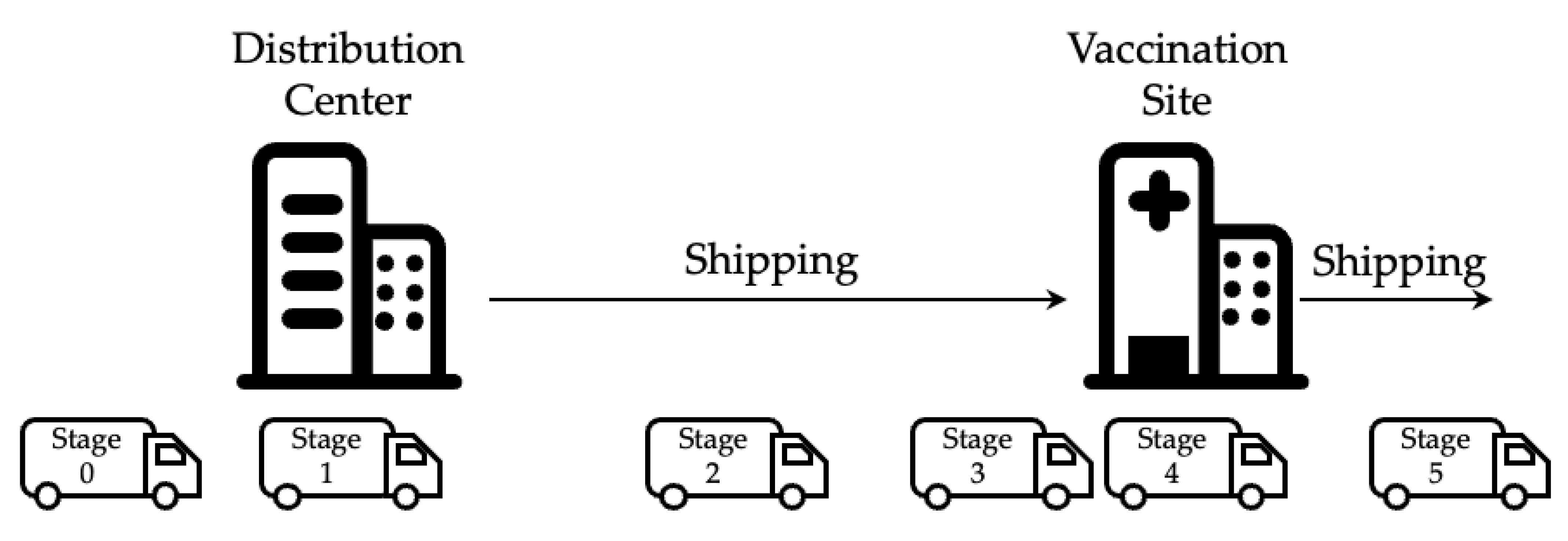
As mentioned previously, vaccines are fragile and unique cargo. We investigate the vaccine distribution process, and the key steps are shown in Figure 1. Figure 1 shows a refrigerated truck departing from a distribution center (DC), serving a customer, and leaving. Stage 0 represents the pre-cooling procedure. Pre-cooling operations are widely used in the cold chain transport industry and are aimed at lowering the temperature inside the car before loading the cargo. According to the cooling performance of the vehicle, the company’s standard operating procedure (SOP) stipulates that the pre-cooling time in summer should not be less than 75 min. Note that the numerical value of 75 min applies only to the vehicles investigated in this paper. Stage 1 is loading. Workers load the vaccine into the compartment at this stage. Stage 2 (Stage 5) denotes shipping. Stage 3 indicates a waiting process. Because each vaccination site has a time window, drivers need to wait if they arrive early. Time windows are very common in the pharmaceutical industry. This is because customers often accept shipments from more than one supplier, and it is difficult for customers to receive service from multiple vehicles at the same time. Therefore, it is necessary to schedule a fixed time window for each supplier. Stage 4 represents the serving (unloading) procedure. In addition, Stage 5 is consistent with Stage 2.

In this paper, we take into account fuel consumption for the model of VRPTW for vaccine distribution. We attempt to plan vaccine distribution routes that consume less fuel from a fleet management perspective. The fuel consumption is generated by cooling the compartment and driving the vehicle and is eventually converted into fuel costs (refrigeration cost and transportation cost). However, complex and unmeasured external factors make the associated fuel consumption difficult to measure. For example, different seasons will result in different fuel consumption. Driver driving habits [2], road conditions [3], and traffic environment will also affect fuel consumption. Therefore, this paper does not use a certain measurement method or monitoring method to finely monitor fuel consumption but uses a series of methods to approximate the fuel consumption. This approach can simplify the objective function of the VRP model without deviating from our intention, making the model easier to be solved. Studies related to fuel consumption measurement systems are reviewed in Section 2. We estimate the fuel consumption of the vehicle per kilometer and consider the pre-cooling provisions in the work specification to evaluate the pre-cooling cost of the vehicle; the other refrigeration costs are calculated based on historical on-board temperature control data and the performance parameters of the refrigeration system.

In addition to fuel consumption, we consider the potential penalty costs in conjunction with the actual business requirements. In reality, drivers often work long hours during the delivery process, increasing the probability of accidents due to drowsy driving. According to a survey by the AAA Foundation for Traffic Safety, one in six fatal crashes and one in eight crashes resulting in hospitalization involve fatigued drivers [4]. Data from European Commission’s Directorate-General for Mobility and Transport shows that for truck drivers, the risk of accidents rises steeply after nine to ten hours of continuous driving. Moreover, when a driver drives for more than four consecutive hours, his driving performance is significantly affected [5]. The loss in case of an accident would be very significant for high-value goods such as vaccines. Another reason that makes us consider penalty costs is balancing the workload of each driver. A single-purpose reduction in fuel costs that increases a driver’s workload or creates an imbalance in the driver’s workload is irrational and detrimental to the company’s growth. Note that our penalty costs are made up of just two factors: the damage caused by a potential accident and the driver’s overtime costs. The penalty cost does not include the driver’s penalty ticket because it is the result of an avoidable human error.

The fuel cost, together with the potential penalty cost, constitutes the total cost, i.e., the objective function of the optimization problem. There is an implicit and soft limit on the working time of each driver. In previous studies, the distance constraint vehicle routing problem (DCVRP) has often been considered. We do not accept distance limits because the driver’s waiting process due to early arrival and the serving time is also part of the working time. However, during waiting and serving customers, the vehicle is not moving. Therefore, it is more accurate to use the working time limit. All the above real-world data comes from a pharmaceutical logistics company with which we form a partnership. The case study part of this paper also comes from a delivery mission of this company in Haidian District, Beijing.

Since VRPTW is an NP-hard problem, the exact method can only be solved in an acceptable computational time for small to medium-scale problems. Therefore, many heuristic and meta-heuristic methods have been proposed to solve real-world size issues. Our model is an extension of VRPTW and is NP-hard also. The higher complexity of the problem and nonlinear objective function leads to the exact methods insufficient to solve large-scale problems in a short time. Therefore, we developed the GA-LNS method to solve the problem. Also, we perform numerical experiments with realistic data in Beijing to investigate the quality of the route, the composition of the costs, and the effect of different parameters on the results.

The paper is organized as follows: Section 2 reviews the relative VRPTW research and the solution methods. Section 3 constructs a mathematical model of the problem. Section 4 designs a GA-LNS method. In addition, Section 5 conducts experiments to show and discuss the results. Finally, Section 6 concludes the paper.

2. Literature Review

As mentioned above, the VRP is a classical OR problem whose related research started in the 1960s [6]. In addition, the VRPTW is an important branch of the VRP [7]. The problem can also be formulated as a linear integer problem with many binary variables [8], which costs exact algorithms a long time to find an optimal solution for a large-scale problem. Thus, heuristics methods are popular in solving VRPTW. In recent years, with the environmental degradation and the gradual increase in the cost of fossil fuels, more and more studies have started to consider fuel consumption in the VRP. A review of the literature on these topics is presented below.

As global environmental awareness has increased in recent years, energy conservation has become an important method for the logistics industry to reduce transportation costs and carbon emissions. Researchers have categorized this issue of environmental considerations in VRPs as Green VRP (GVRP). Ghorbani et al. investigate the issue of environmentally friendly VRP [9]. Asghari and Al-e-hashem provide an overview of the recent progress in the research of GVRP [10]. In the study of VRP, in which vehicles are driven by conventional fossil fuels, fuel consumption is a very important factor [11]. Bektaş et al. consider more factors for the objective function of VRP [12], including routes, greenhouse gas emissions, energy consumption, etc. In GVRP, energy consumption is usually assumed as a function of travel distance or travel time [13]. However, the reality is complex, and factors such as vehicle speed [14], road conditions [3,15,16], and driving habits [2] affect the fuel consumption of the vehicle. Xiao et al. developed a pollution routing model considering driving speeds, travel times, arrival/departure/waiting times, and vehicle loads [17].

This paper investigates the energy consumption of conventional fuel-powered trucks, and we also pay attention to the studies of the energy consumption of electric vehicles. Li et al. study the VRP problem for electric vehicles based on battery swapping [18]. Seyfi et al. consider different driving modes in route planning for hybrid electric vehicles with electric engines and internal combustion engines [19]. Noting that our problem is related to refrigerated trucks, there are studies on a VRP of the refrigerated truck as follows. Ceschia et al. extend the VRP for refrigerated trucks by considering the effect of the time factor on the objective function in the model [20]. Chen et al. explore the VRP for fresh food with an objective function that considers fixed cost, fuel cost, and penalty cost [21]. They develop a TS algorithm to solve the problem at a real-world scale. Meneghetti and Ceschia construct a mathematical model for cold chain distribution [22]. Their study considers the temperature variation and the gas tightness of the compartment. Habibur Rahman et al. build a model for fuel consumption in the cold chain with the goal of reducing carbon emissions [23]. Zhang et al. explore fuel consumption and carbon emissions in VRP, assuming that fuel consumption is related to the loading of the vehicle on the route [24]. They customize a tabu search algorithm to solve this problem. Li et al. minimize the total cost (including refrigerating cost, fixed cost, and transportation cost) of cold-chain drug distribution in a certain region, establish a DCVRP optimization model, and develop a tabu search algorithm to solve the model [25].

In addition, issues concerning fuel consumption have received much attention. Zhou et al. reviewed related fuel consumption models [26]. Peng and Ma establish a new model to evaluate the fuel consumption on the highway [27]. Another part of the research focuses on the prediction of oil consumption using new techniques, such as artificial neural networks (ANN) [28], backpropagation (BP) neural networks [29], and the support vector machine (SVM) [30]. Anyway, the use of Onboard Diagnoses (OBD) as a monitoring tool is one of the important methods for studying fuel consumption [30,31]. The fuel consumption of the vehicle is also related to the type of vehicle. Yu et al. investigate the fuel consumption of heavy-duty commercial vehicles [32]. In comparison, Zheng et al. studied the fuel consumption of light-duty passenger vehicles [33].

VRPTW is one of the best-known and most attractive variants of classical VRP research. Every year hundreds of works of scientific literature on VRP variants or branches are published, which is mostly related to solution algorithms [34,35]. Zhang et al. investigate and review the VRPs and the solving methods [36]. Currently, the mainstream methods for solving VRPTW problems are mainly classified into exact and heuristic methods. Machine learning is also considered a promising research topic for solving VRP problems [37]. Baldacci et al. provide a review of exact algorithms for solving VRPTW [38]. Gendreau and Tarantilis [39] and Awd and Elshaer [34] review and summarize metaheuristic algorithms for solving VRPTW. The main well-performing metaheuristic algorithms for solving VRPTW include GA [40,41], LNS [42], simulated annealing (SA) [43], memetic algorithm (MA) [44], tabu search (TS) [45], ant colony optimization (ACO) [46], particle swarm optimization (PSO) [47], etc.

In our literature review, there are few VRP models for fuel consumption based on the vaccine distribution process. In Section 3, a VRPTW model for vaccine distribution was constructed to evaluate fuel consumption during vaccine distribution.

3. Mathematical Model

In this section, we will construct a nonlinear integer programming model for VRPTW. Before constructing the model, we define some notations based on graph theory. Note that the base VRPTW model is given by Cordeau et al. [48], and we expand on it. The model of VRPTW for vaccine distribution is on a complete graph $G=\left(V,A\right)$, where $V=\left\{0,1,\dots ,n,n+1\right\}$ is the vertex set and $A=\left\{\left(i,j\right)|i\in V,j\in V\right\}$ is the arc set. Node index $0$ and $n+1$ denote the departure point and return point of the DC separately. Subset$N=\left\{1,\dots ,n\right\}\subseteq V$ represents the customer set. A time window $\left[e_i,l_i\right]$ is associated with a vertex $i\in V$, where $e_i$ is the lower bound of the time that allowed to serve $i$ (i.e., the earliest time) while $l_i$ is the upper bound (i.e., the latest time). Meanwhile, a demand $d_i$ and a service time $s_i$ are associated with the vertex $i\in V$. Each arc $\left(i,j\right)\in A$ has a corresponding and a travel time $t_{ij}=\frac{D_{ij}}{v}$, where $D_{ij}$ is the distance between node $i$ and node $j$ and $v$ is the average speed. The truck set is denoted by $K$, where a homogeneous truck $k\in K$ has the maximum capacity $C$. In order to facilitate modeling, all trucks must depart from DC (index $0$) and return DC (index $n+1$). To indicate the order of visiting customers, ${\mathsf{\Delta }}^{+}\left(i\right)=N\backslash \left\{i,n+1\right\},\forall i\in V$ denote the vertexes can be visited before $i$, while ${\mathsf{\Delta }}^{-}\left(i\right)=N\backslash \left\{i,0\right\},\forall i\in V$ denote the vertexes can be visited after $i$.

In addition, the time window of the DC means that the working hours of the DC, which is denoted by$\left[e_0,l_0\left]=\right[e_{n+1},l_{n+1}\left]=\right[E,L\right]$, where $E$ and $L$ are the lower and upper bound of the time in this problem, respectively. Particularly, the travel time between the departure point and return point without visiting any other customer is 0 (i.e., $t_{0,n+1}=0$), and the demands of the DC equal 0 (i.e., $d_0=d_{n+1}=0$). Binary decision variables $x_{ijk}$, equal 1 if truck $k\in K$ visit vertex $j\in V$ from vertex $i\in V$, and 0 otherwise. In addition, continuous variables $w_{ik}$ denote the arrival time of the truck $k\in K$ to $i\in V$. For the convenience of the reader, all notations and interpretations are in

Table 1. Notation list.

Parameter	Description
VRPTW Parameter
$G$	General graph
$V$	Set of vertexes
$A$	Set of arcs
$N$	Set of customers
$K$	Set of Trucks
$e_i$	Earliest time for node $i$
$l_i$	Latest time for node $i$
$E$	Earliest time for DC
$L$	Latest time for DC
$s_i$	Service time for node $i$
$d_i$	Demands for node $i$
$v$	Average speed
$t_{ij}$	Travel time for arc $\left(i,j\right)$
$D_{ij}$	Distance for arc $\left(i,j\right)$
$C$	Capacity for truck
${\mathsf{\Delta }}^{+}\left(i\right)$	Vertexes can be visited before $i$
${\mathsf{\Delta }}^{-}\left(i\right)$	Vertexes can be visited after $i$
Case Parameter
$C_t$	Transportation cost
$C_{r1}$	Pre-cooling cost
$C_{r2}$	Waiting and transportation refrigeration cost
$C_{r3}$	Service refrigeration cost
$C_p$	Penalty cost
$C_{total}$	Total cost
$\mu$	Fuel consumption per kilometer consumed by the truck
$\alpha$	Price per unit of fuel
$P$	Rated power input of the refrigeration system
$Q$	Calorific value per unit of fuel
$\eta$	Efficiency of converting fuel energy into heat energy
$T_{cool}$	Duration of pre-cooling process
$T_{lim}$	Standard working hour
$\kappa$	Ratio of the cooling time to the waiting and traveling time
$\pi$	Penalty cost per hour
Decision Variable
$x_{ijk}$	$x_{ijk}=1$ denotes truck $k$ visit $j$ after $i$, and $x_{ijk}=0$ otherwise.
$w_{ik}$	Arrival time of truck $k\in K$ to $i\in V$

.

As mentioned earlier, the objective function of the VRPTW for vaccine distribution is to minimize the total cost, including fuel cost and penalty cost. Fuel costs can be further subdivided. The costs incurred by using fuel to drive a vehicle are defined as transportation costs, and the costs incurred by using fuel to reduce the temperature of the compartment are defined as refrigeration costs. In order to calculate the transportation cost and the refrigeration cost, we evaluate the fuel consumption by referring to the thermodynamic theory and historical data. The consumption is then multiplied by the cost per unit of fuel and the carbon tax. The objective function is derived and formulated as follows:

We consider transportation costs as a linear function of distance. There are several reasons for this consideration: First, we can estimate the transportation cost per kilometer by projecting the fuel consumed per kilometer of truck travel based on drivers’ empirical data. Second, for small trucks in urban distribution, the fuel consumption is not very much related to the loading capacity, i.e., empty and full loads do not have a particularly large impact on the fuel consumption per kilometer. Next, in practice, people often use fuel consumption per kilometer to measure the fuel consumption level of trucks. Finally, most VRP models idealize transportation costs as a linear function of distance, and we adopt this assumption. Defining the fuel consumption per kilometer consumed by the truck driving as $\mu$, the transportation cost as $C_t$, the price per unit of fuel as $\alpha$. The expression for the transportation cost $C_t$ is shown in Equation (1).

$$C_t=\alpha \mu {\displaystyle \sum _{k\in K}}{\displaystyle \sum _{\left(i,j\right)\in A}}{D}_{ij}{x}_{ijk}$$

(1)

The refrigeration costs comprise pre-cooling costs, waiting and transportation refrigeration costs, and service refrigeration costs. Before the refrigerated truck is loaded, the temperature inside the compartment needs to be lowered to the specified temperature for further operation. Currently, the refrigeration system runs at maximum power to make the temperature inside the compartment drop rapidly. The truck’s refrigeration system is powered by the truck’s engine, which converts internal energy into mechanical energy by burning fuel and then drives the generator to work. The efficiency of converting fuel energy in the engine into heat energy in the refrigeration system is $\eta$. If the temperature inside the car meets the requirements, the pre-cooling process is finished. According to the SOP, the duration of pre-cooling is clearly defined, although it varies with the season. Define the duration of the pre-cooling process is $T_{cool}$, rated power input of the refrigeration system is $P$, and the calorific value per unit of fuel is $Q$. The pre-cooling cost of the truck $C_{r1}$ is calculated in Equation (2).

$$C_{r1}=\frac{\alpha P{T}_{cool}}{Q\eta }{\displaystyle \sum }_{k\in K}{\displaystyle \sum }_{j\in N}{x}_{0jk}$$

(2)

Waiting and transportation refrigeration costs are due to poor truck containment and insulation, which in turn generates cooling air loss. In order to prevent the temperature inside the car from rising, the truck needs to maintain the temperature while waiting and traveling. In practice, truck temperatures are often human-controlled, and it is very difficult to accurately measure the refrigeration costs of transport and waiting due to the complexity of the situation. However, we can estimate from the temperature control data and historical data of the truck. The temperature change of the inside compartment shows a certain regular trend. The starting temperature of the truck is maintained between the upper and lower temperature bounds. Then, in order to save energy, the driver will turn off the refrigeration system causing the truck temperature to rise. When the temperature inside the truck approaches the upper temperature bound, the refrigeration system is turned on again. When the temperature drops to the lower temperature bound, the system is turned off again. Thus, the temperature curve of the truck shows an up-and-down trend (jagged). Define $\kappa$ as the ratio of the cooling time to the waiting and traveling time. Note that the denominator of this ratio is not the total operating hours. This is because the cooling operation in loading and unloading is different from the cooling operation in traveling or waiting. This will be described later. Equation (3) calculates the waiting and transportation refrigeration cost $C_{r2}$.

$$C_{r2}=\frac{\alpha P\kappa }{Q\eta }\left({\displaystyle \sum }_{k\in K}{\displaystyle \sum }_{\left(i,j\right)\in A}{t}_{ij}{x}_{ijk}+{\displaystyle \sum }_{j\in V}\max \left\{{\displaystyle \sum }_{k\in K}{\displaystyle \sum }_{i\in V}{x}_{ijk}\left(e_j-w_{ik}-s_i-t_{ij}\right),0\right\}\right)$$

(3)

Service refrigeration costs represent the cost of the truck to compensate for the increase in compartment temperature caused by opening the compartment door while serving the customer. Each customer has cold storage to store vaccines. In order to ensure that the vaccines are in a constant temperature environment throughout, the compartment is docked with the customer’s storage door and has an airtight device to minimize cold air leakage. Usually, when serving a customer, the compartment’s refrigeration system is in operation to prevent the temperature from exceeding the upper limit. Since the compartment is connected to the depot, the excess cold air that the refrigeration system creates will flow into the storage and will not cause the interior temperature of the compartment to become too low. Therefore, the service refrigeration cost $C_{r3}$ is shown in Equation (4).

$$C_{r3}=\frac{\alpha P}{Q\eta }{\displaystyle \sum }_{i\in V}{s}_i$$

(4)

Penalty costs are incurred when drivers work more than the maximum working hours. Considering the high value of the goods delivered, the pharmaceutical logistics company does not want a driver to work too many hours, which can lead to fatigue and threaten the safety of the vaccines. In addition, a penalty cost is set in order to equalize the working hours of each driver in the optimization process. This cost can be considered as an overtime payment for drivers or as a loss due to potential accident risk. The penalty cost per hour over the standard working hour limit $T_{lim}$ is $\pi$. The penalty cost $C_p$ is calculated in Equation (5).

$$C_p=\pi {\displaystyle \sum }_{k\in K}\max \left\{w_{n+1,k}-w_{0k}-T_{lim},0\right\}$$

(5)

In summary, the total cost of VRPTW for vaccine distribution $C$ is calculated in Equation (6).

$$C_{total}=C_t+C_{r1}+C_{r2}+C_{r3}+C_p$$

(6)

With objective function, the model of VRPTW for vaccine distribution can be formulated as follows:

$$\min C_{total}$$

(7)

$${\displaystyle \sum }_{\mathrm{k}\in \mathrm{K}}{\displaystyle \sum }_{j\in {\mathsf{\Delta }}^{+}\left(i\right)}{x}_{ijk}=1,\forall i\in N$$

(8)

$${\displaystyle \sum }_{j\in {\mathsf{\Delta }}^{+}\left(0\right)}{x}_{0jk}=1,\forall k\in K$$

(9)

$${\displaystyle \sum }_{i\in {\mathsf{\Delta }}^{-}\left(n+1\right)}{x}_{i,n+1,k}=1,\hspace{0.17em}\hspace{0.17em}\forall k\in K$$

(10)

$${\displaystyle \sum }_{i\in {\mathsf{\Delta }}^{-}\left(j\right)}{x}_{ijk}={\displaystyle \sum }_{i\in {\mathsf{\Delta }}^{+}\left(j\right)}{x}_{jik},\hspace{0.17em}\hspace{0.17em}\forall k\in K,\hspace{0.17em}j\in N$$

(11)

$$x_{ijk}\left(w_{ik}+s_i+t_{ij}-w_{jk}\right)\le 0,\forall k\in K,\left(i,j\right)\in A$$

(12)

$$e_i{\displaystyle \sum }_{j\in {\mathsf{\Delta }}^{+}\left(i\right)}{x}_{ijk}\le w_{ik}\le l_i{\displaystyle \sum }_{j\in {\mathsf{\Delta }}^{+}\left(i\right)}{x}_{ijk},\forall k\in K,\mathrm{i}\in N$$

(13)

$$E\le w_{ik}\le L,\forall k\in K,\mathrm{i}\in \left\{0,\mathrm{n}+1\right\}$$

(14)

$${\displaystyle \sum }_{i\in N}{d}_i{\displaystyle \sum }_{i\in {\mathsf{\Delta }}^{+}\left(j\right)}{x}_{ijk}\le C,\forall k \in K$$

(15)

$$D_{ij}=v{t}_{ij},\forall \left(i,j\right)\in A$$

(16)

$$x_{ijk}\in \left\{0,1\right\},\forall \left(i,j\right)\in A,\forall k\in K$$

(17)

$$w_{ik}>0, \forall i\in V, k\in K$$

(18)

The objective function (7) is to minimize the total cost. Constraints (8) stipulate that each customer can only be served by one truck. Constraints (9) and (10) require all trucks to depart from and return to DC. Constraints (11) characterize the inflow and outflow of nodes are equal. Constraints (12)–(14) ensure that time requirements are met. Constraints (15) is the capacity limitation. Constraints (16) are the relationship between shipping time and distance. Constraints (17) and (18) are the decision variables.

4. GA-LNS Method

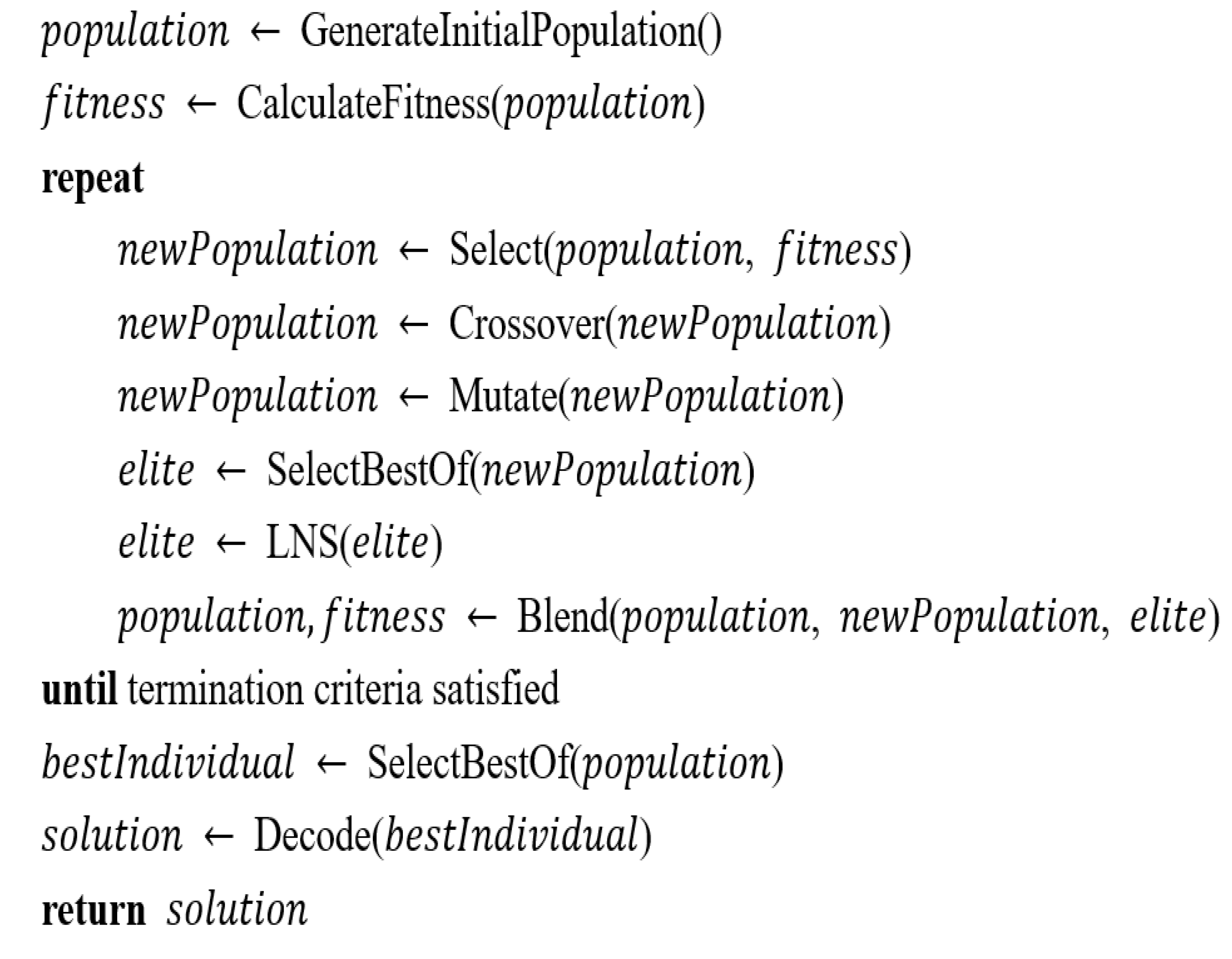
This section describes the GA-LNS algorithm for addressing VRPTW for vaccine distribution, where LNS is embedded as an operator in the framework of GA to improve the quality of the solution. GA is a population-based evolutionary algorithm that draws on the ideas of natural selection and genetic recombination. As in nature, in a standard GA, the basic unit of evolution is the population containing a set of individuals. Each individual in the population represents a particular solution to the problem to be solved, i.e., the population is a set of solutions. The process of converting a particular solution to the problem into some representation of an individual by means of certain rules is called encoding. In turn, the process of converting an individual into a solution to the problem is called decoding. Since the quality of the solution represented by each individual in the population differs, to represent this difference, fitness value is used to measure the viability of an individual and the quality of the corresponding solution. The higher the fitness of an individual, the better the quality of the solution it represents, and the more likely it is to pass on its properties to the next generation during the evolutionary process. An evolutionary cycle of a population is called a generation and contains selection, crossover, and mutation operations. These operations are computed on the population, mimicking the natural reproduction process, where two individuals are selected according to fitness crossover and produce new individuals. In addition, similar to nature, individuals also mutate with a certain probability. These mutations may result in individuals with higher fitness or may enrich the diversity of the population. In fact, GA is also a stochastic optimization algorithm, and the above-mentioned crossover and mutation operations are essentially discovering possible better solutions in the solution space. However, the ability of GA’s search is limited. In order to enhance the search capability and improve the solution quality, the LNS operator is embedded in the GA to form a GA-LNS to further discover possible better solutions. In addition, for the VRPTW problem, we introduce the TSP-split encoding approach is introduced into GA-LNS. Prins et al. review the studies related to this encoding approach [49].

The principle of GA was proposed by Holland [50]. With continuous improvements in recent decades, GA has achieved rich results in solving the VRPTW and is the most popular evolutionary algorithm for solving VRPTW [34]. For more details on GA and advanced GA, see Whitley [51]. The pseudo-code of our GA-LNS algorithm is shown in Figure 2. Details of each operator are presented in subsequent subsections.

4.1. Encoding Method: TSP-Split

The TSP-split encoding method is an Order-first split-second method. The core principle of this encoding method was proposed by Beasley [52]. First, similar to solving the TSP problem, the coding process relaxes the vehicle capacity constraint and the customer time window constraint to construct all customers into one giant tour, which is composed of all customer numbers without any route separators. In general, it is usually impossible to use only one truck to serve all customers on tour. Therefore, it is necessary to cut the giant tour into several segments, each served by a truck. Second, the cutting problem is equated to the shortest path problem by making an auxiliary diagram, and the split algorithm cuts the tour into the vehicle route with the minimum total cost in polynomial time. With a sufficient number of vehicles, the method always keeps the coding length constant and guarantees that all the paths obtained by the split algorithm are feasible. We encode all the vaccination sites into a giant tour without separators and then use a splitting algorithm to split this large loop into vehicle routes. The TSP-split method is described as follows.

Given a giant tour $S$ consisting of a node-set $V$. The giant tour $S$ can be optimally split into $S\left(m\right)$ sections (where integer $m\ge 1$), and each segment can be converted into a vehicle route by adding DC before and after the segment. Define the fixed cost of the vehicle as $F=\frac{\alpha P{T}_{cool}}{Q\eta }$ [the fixed cost is the pre-cooling cost, i.e., the coefficient in Equation (2)] and the generalized transportation cost $C_t^g\left(i,i+1,\dots ,j\right)$ as equal to the cost associated with the transportation process (generalized transportation cost is the sum of transportation cost, waiting and transportation refrigeration cost, service refrigeration cost, and penalty cost) for the route $\langle 0,i,i+1,\dots ,j,n+1\rangle$.

Define the auxiliary graph $G_H=\left(V^{\prime },Y,W\right)$, where $V^{\prime }=V\backslash \left\{n+1\right\}$ is the set of points in $G_H$, $Y$ is the set of arcs containing arcs $\left(i,j\right),\forall i\in V,\forall j\in V,i<j$, and $W=\left\{w_{ij}\right|\left(i,j\right)\in Y\}$ is the set of weights of arcs. The weight of the arc $\left(i,j\right)\in Y$, $w_{ij}$ is calculated by the following Equation (19):

$$w_{i,j}=F+C_t^g\left(i+1,\dots ,j\right)$$

(19)

Under the time window and capacity constraints, the weight for an arc between node $i$ and node $j$ in $G_H$ equals to the total cost calculated in Equation (19) for the route $\langle 0,i+1,\dots ,j,n+1\rangle$. If route $\langle 0,i+1,\dots ,j,n+1\rangle$ does not satisfy the constraints, then delete the corresponding arc or let the equal weight infinity. Then, use the shortest path algorithm (Dijkstra’s algorithm or Bellman-Ford algorithm) to find the shortest path from node 0 to point $n$ in the graph$G_H$. The distance for the shortest path problem for node 0 and node $n$ in $G_H$ is the objective function value under this big tour. In addition, the arcs included in the shortest path can be resolved backward into vehicle routes.

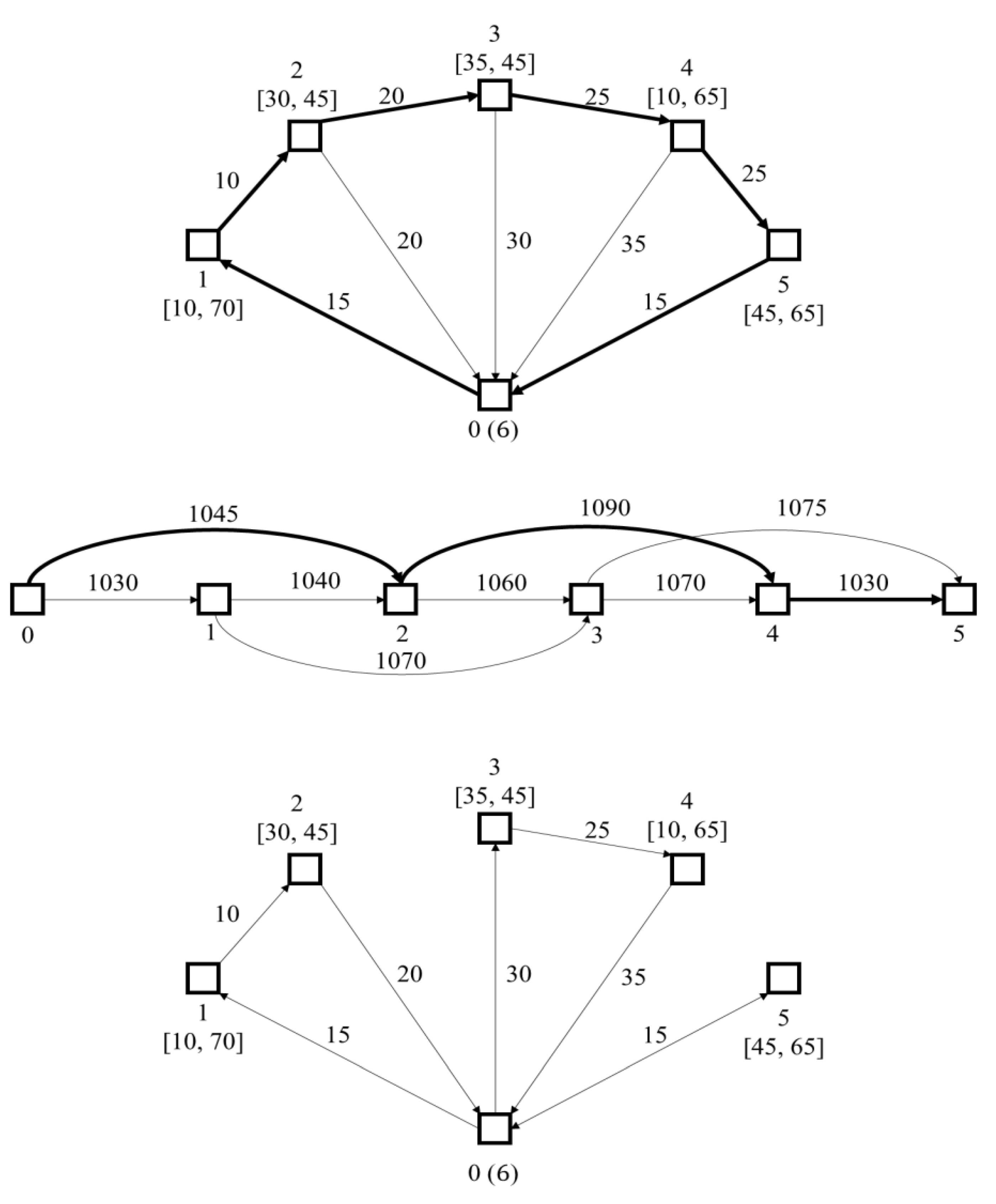
To represent the above encoding method in a concrete way, we introduce the big tour in the upper part of Figure 3. Similar examples can be found in [49,53]. In this example, to simplify the illustration, let $C_t^g\left(i,i+1,\dots ,j\right)$ equals to the total distance for the route $\langle 0,i,i+1,\dots ,j,n+1\rangle$. In addition, set $s_i=0,\forall i\in V$, $F=1000$, and relax the capacity constraints. In the upper part of Figure 3, the giant tour consisting of DC indexed by $0$ or $6$ and all customers indexed by $1$ to $5$ is indicated by the bolded line. The number next to the arc is the distance between the two nodes. In addition, the number in square brackets is the time window corresponding to the customer.

Auxiliary graph $G_H$ is in the middle part of Figure 3. The numbers next to the arcs indicate the weights. According to Equation (18), the weight of arc $\left(1,2\right)$, $w_{12}$ equals the total cost of the route $\langle 0,2,6\rangle$, and $w_{24}$ equals the total cost of the route $\langle 0,3,4,6\rangle$, similarly. However, there is no arc $\left(0,3\right)$ in $G_H$, since the time to reach customer $3$ after customers $1$ and $2$ in the giant tour exceeds the latest time for customer 3.

The shortest path from node 0 to node 5 in $G_H$ (the bolded arcs in the middle part of Figure 3) can be obtained using the shortest path algorithm, i.e., the minimum cost under this giant tour is 3165, meaning that the giant tour can be split into three routes with a minimum distance of 3165. All arcs in the shortest paths can be resolved backward into vehicle routes, i.e., three vehicles are used, the first vehicle serves customer 1 and 2, the second serves 3 and 4, and the third serves customer 5. The vehicle routes are shown in the lower part of Figure 3.

4.2. Initial Solution

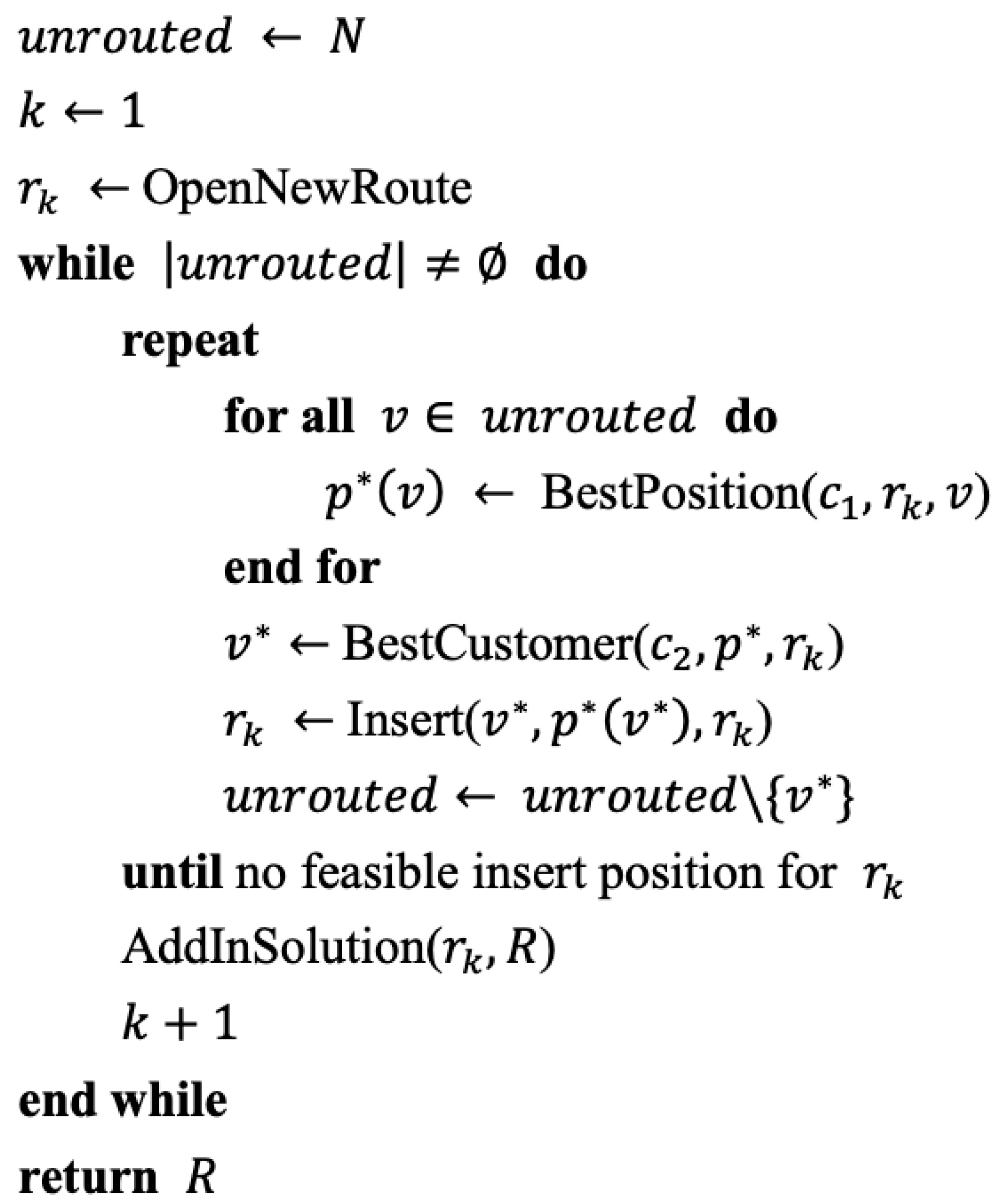
In order to generate an initial solution for this problem, we adopted the Solomon Insertion I1 heuristic, the principle of which was proposed by Solomon [54]. The insertion heuristic I1 generates feasible vehicle routes by inserting customers one by one in the initial route under the time window and capacity constraints. We use the Solomon Insertion I1 heuristic to generate the initial solution, focusing on its feasibility. Define a route $r=\langle 0,v_1,\dots ,v_m,n+1\rangle$, containing $m$ ($0\le m\le \left|N\right|$) customers. The pseudocode of insertion I1 heuristic is as shown in Figure 4.

Let the solution to the problem consist of the set of routes of the vehicle as $R=\left\{r_k\right|k\in K\}$, which contains $k$ vehicle routes, each of which is $r_k$. Solomon Insertion I1 heuristic opens a new and empty route $r_k=\langle 0,n+1\rangle$ and inserts the unrouted customers into a feasible position in the route according to two criteria. The first criteria $c_1$ determines the best insert position for each customer, and the second criterion $c_2$ determines which customer will be inserted. After inserting unrouted customer $v$ in the route $r_k=\langle 0,v_1,\dots ,v_{p-1},v_p,\dots ,v_m,n+1\rangle$ at $p$, update $r_k=\langle 0,v_1,\dots ,v_{p-1},v,v_p,\dots ,v_m,n+1\rangle$. The best inserting position $p^{\ast }$ for customer $v$ is evaluated as follows:

$$p^{\ast }=\arg \underset{p=1,\dots ,m}{\min }{c}_1\left(v_p,v,v_{p+1}\right)$$

(20)

$$c_1\left(i,v,j\right)=\phi c_{11}\left(i,v,j\right)+\varphi c_{12}\left(i,v,j\right)$$

(21)

$$c_{11}\left(i,v,j\right)=D_{iv}+D_{vj}-\rho D_{ij}$$

(22)

$$c_{12}\left(i,v,j\right)=w_{jk}^{new}-w_{jk}^{old}$$

(23)

$$\phi +\varphi =1, \phi \ge 0,\varphi \ge 0,\rho \ge 0$$

(24)

Equation (20) is the optimal insertion position of unrouted customer $v$ in the route and the criterion $c_1$ of Equation (21) denotes the weighted sum of the increased distance (Equation (22)) and the increased time (Equation (23)). Parameter $w_{jk}^{new}$ is the new arrival time for truck $k$ visiting $j$ after the insertion, while the $w_{jk}^{old}$ is old before insertion. Notations $\phi$, $\varphi ,$ and $\rho$ are the parameters for calculating the increment after insertion.

Then, according to the $c_2$ criterion in Equation (26), the most suitable unrouted customer $v^{\ast }$ [Equation (25)] maximize $c_2$ criterion will be inserted in the feasible position of the route. The formula of the $c_2$ criterion is as follows, in which $\theta$ is the parameter weighting the distance between DC and customer $v$.

$$v^{\ast }=\arg \underset{v\in \mathrm{Unrouted}\wedge \mathrm{Feasible} \mathrm{insert}}{\max }{c}_2\left(v_{p^{\ast }\left(v\right)}, v, v_{p^{\ast }\left(v\right)+1}\right)$$

(25)

$$c_2\left(i,v,j\right)=\theta D_{0v}-c_1\left(i,v,j\right)$$

(26)

$$\theta \ge 0$$

(27)

Repeat the above steps to keep inserting unrouted customers into the route. When no feasible insertion position exists for the route, close the route and add it to $R$. If there are still unrouted customers, open a new route and repeat the insertion process until there are no unrouted customers.

Obviously, with the default values of the parameters $\phi$, $\varphi$, $\rho ,$ and $\theta$, only one initial solution can be generated by this method. To enhance the diversity of the population, we fix the parameters $\rho$ and $\theta$, and the parameters $\phi$ and $\varphi$ vary with the order of the current individual in the population. Define the constant population size as $Z$ and the index of the current individual in the population as $z$. Then, the value of $\phi$ for individual $z$ is equal to $z/Z,$ and the value of $\varphi$ is equal to $1-z/Z$. Note that the Solomon insertion I1 heuristic only generates feasible solutions to this model without considering the quality or the objective value. The process of finding better solutions will be conducted by the GA operators shown below.

4.3. GA Operators

4.3.1. Evaluation of Fitness

For the individuals in the population, after decoding, they can be converted into the values of the decision variables in the model, which in turn gives the objective function values in Equation (7). Since the problem to be solved is a minimization problem, the smaller the value of the objective function, the higher the fitness of the corresponding individual in the population. We used the relative fitness approach, which is related only to the objective function value of the individuals in the current generation. The fitness value of each individual in the population is equal to the minimum objective function value in the whole population divided by the objective function value of each individual, i.e., the relative fitness is between 0 and 1.

4.3.2. Selection Operator

Roulette wheel selection is one of the most used selection methods in which the probability of an individual being selected is proportional to the fitness value of the individual. In general wheel roulette selection, there is only one pointer, which may lead to multiple selections of the same individual with higher fitness, making the population less diverse. To solve such a problem, we use a stochastic universal sampling (SUS) method [55]. This method improves the roulette wheel selection by adding equally spaced pointers. The number of pointers is determined by a parameter $P_s$ called generation gap between 0 and 1, i.e., the number of selected individuals that have the opportunity to pass their attributes to their offspring is equal to $\left[Z{P}_s\right]$, where $\left[·\right]$ is a rounding operator.

4.3.3. Crossover and Mutation

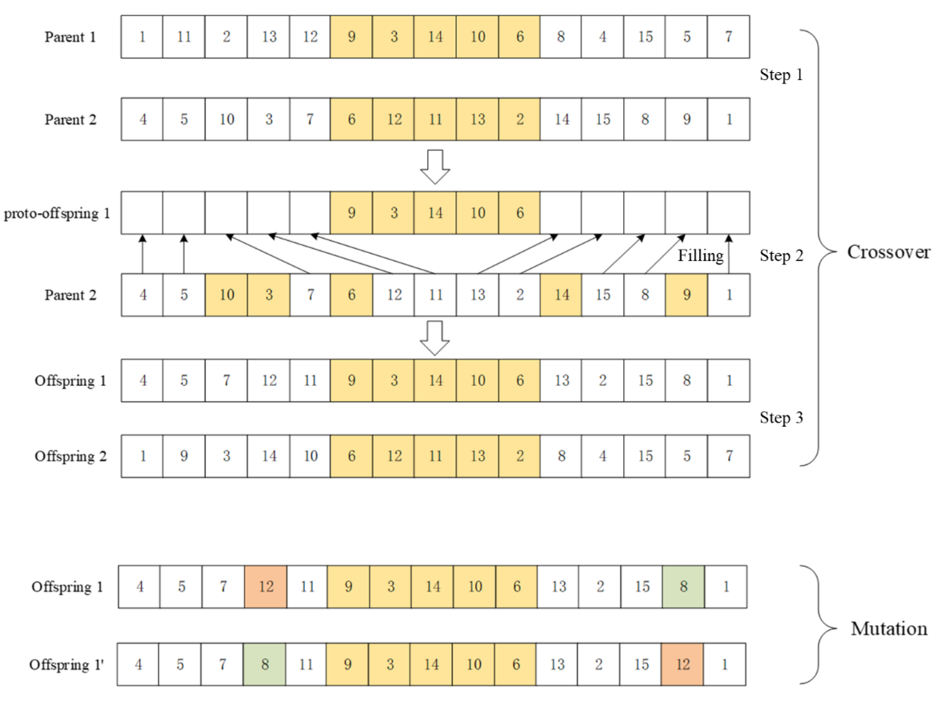
The GA operator includes crossover and mutation, where chromosomes are crossed over and mutated with probabilities of $P_C$ and $P_M$, respectively. There are many crossover operation methods in GA, and Order Crossover (OX) is often applied to VRPTWs because the OX operation can maintain the continuity of gene fragments even when chromosomes are crossed. The process of OX operation is as follows:

Step 1.

Two individuals are randomly selected as parents from the selected population. They intercept a segment of genes at the same position, as shown in the yellow parts of Parent 1 and Parent 2 in the upper of Figure 5.

Step 2.

The proto-offspring1 inherits the yellow gene from Parent 1, and the rest of the genes (the white) are provided by Parent 2. We identify the position of the yellow gene in Parent 2, fill the rest of the genes in order in the proto-offspring 1, and avoid the formation of the above position in Offspring 1.

Step 3.

By the same principle in STEP 2, Offspring 2 is formed.

The mutation operator in the GA for the VRPTW is conventional, requiring only a random swap of the positions of two genes on the same chromosome (the lower part of Figure 5 for the orange and green genes).

4.3.4. Blend Parents and Offspring

After the selection, crossover, and mutation operator calculations, we obtain the child population and the parent population, which will have a total size greater than $Z$. In order to keep the population size constant, the blend operation merges the two populations and then removes duplicate individuals. If the size of the population after de-duplication is larger than $Z$ then the first $Z$ individuals in descending order of fitness are taken. Otherwise, the insertion heuristic is used for supplementation.

4.3.5. Termination Criteria

The termination criterion of GA is related to the maximum generation $M_{iter}$. If this parameter is too large, it causes the algorithm to take too long to compute. If this parameter is too small, it leads to poor solution quality. The GA terminates when it satisfies the following two criteria:

• The ratio of the number of iterations in which the objective function is not improved to the maximum number of generations $M_{iter}$ exceeds the parameter $\beta$ .
• The iteration reaches $M_{iter}$.

4.4. LNS Operator

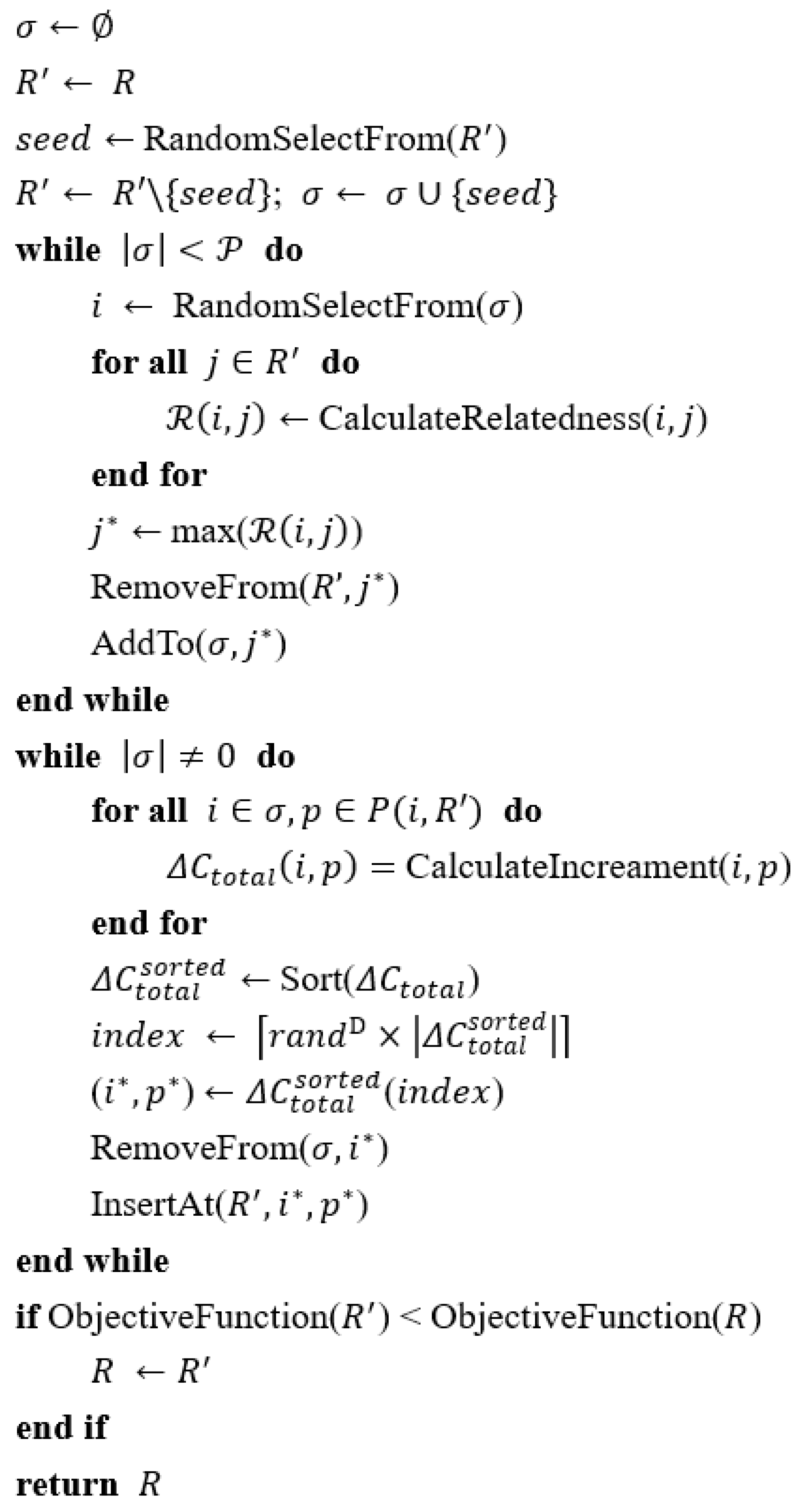
In fact, the classical GA described above can already obtain an optimized feasible solution. In order to obtain an improved solution, the LNS operator is introduced. The LNS method was proposed by [56], which acts on a solution and thus can be embedded in a GA to improve the quality of the solution. We adopt elitism, i.e., we target only the elite chromosomes in the population for the LNS operation. LNS belongs to a type of neighborhood search heuristic, which generates neighborhoods by a destroy method and a repair method. The destroy method removes customers from the solution according to certain rules and randomness. The repair method reinserts the unrouted customers into the routes by greedy strategies and randomness to possibly produce a better solution. If the newly generated solution is better than the original solution, the original solution is replaced and searched again. The pseudo-code of the neighborhood search operator algorithm is shown in Figure 6.

Shaw designed relatedness-based destroy rules for the LNS algorithm of VRPTW Shaw [56]. Two customers are more related if they are close to each other on the graph or if two customers are served by the same vehicle. The customers moved out by this rule will be in a certain area. The repair operation then reinserts the customers in this area to produce a better solution. Let $\sigma$ denote the set of unrouted customers, and $\mathcal{P}$ denote the maximum number of unrouted customers. The operation to remove customers from the current path $R$ of a vehicle is as follows:

Step 1.

Set $\sigma =\varnothing$ and $R’=R$.

Step 2.

A customer is randomly moved as a seed in $R’,$ and that customer is added to $\sigma$.

Step 3.

Randomly select a customer $i$ in $\sigma$ and calculate the relatedness $\mathcal{R}\left(i,j\right)$ between all customers $j\in R^{\prime }$ and $i$.

Step 4.

The customer $j^{\ast }$ with the highest relatedness with $i$ is removed from $R’$ and added to $\sigma$.

Step 5.

Stop if $\left|\sigma \right|=\mathcal{P}$ and return to Step 2 if $\left|\sigma \right|<\mathcal{P}$.

Equation (28) defines the relatedness of two customers, and the calculation of relatedness $\mathcal{R}\left(i,j\right)$ requires two parameters: The normalized distance is calculated as shown in Equation (29). In addition, the vehicle binary judgment parameter is shown in Equation (30). When customers $i$ and $j$ are served by the same vehicle, the judgment parameter $f_{ij}=0$, otherwise it is equal to 1.

$$\mathcal{R}\left(i,j\right)=\frac{1}{d_{ij}^{’}+f_{ij}},\forall i\in \sigma ,\forall j\in R^{\prime }$$

(28)

$$d_{ij}^{’}=\frac{d_{ij}}{\underset{j^{\prime }\in \mathrm{R}}{\max }{d}_{i{j}^{\prime }}},\forall i\in \sigma ,\forall j\in R^{\prime }$$

(29)

$$f_{ij}=\left\{\begin{array}{c}0, \mathrm{if} i \mathrm{and} j \mathrm{are} \mathrm{served} \mathrm{by} \mathrm{the} \mathrm{same} \mathrm{vehicle}\\ 1, \mathrm{otherwise}\hfill \end{array}\right.$$

(30)

The repair method uses a greedy strategy to insert $\mathcal{P}$ customers of $\sigma$ into the routes one by one. During each insertion, the current objective function value increases with the insertion of clients. Define $P\left(i,R’\right)$ to be the set of feasible insertion positions of client $i\in \sigma$ in the routing plan $R’$. Let $\mathsf{\Delta }{C}_{total}\left(i,p\right)$ denote the increment of the objective function after inserting customer $i$ into the feasible position $p\in P\left(i,R’\right)$. The steps of the insertion operation are detailed as follows.

Step 1.

Calculate the increment of all objective functions $\mathsf{\Delta }{C}_{total}\left(i,p\right),i\in \sigma ,p\in P\left(i,R’\right)$.

Step 2.

Select the customer $i^{\ast }$ and the corresponding feasible position $p^{\ast }$ that minimizes the increment of the objective function, i.e., $\left(i^{\ast },p^{\ast }\right)=\arg \underset{i\in \sigma ,p\in P\left(i,R^{\prime }\right)}{\min }\Delta C_{total}\left(i,p\right)$.

Step 3.

Insert $i^{\ast }$ at $p^{\ast }$, update $R’$ and remove $i^{\ast }$ from $\sigma$.

Step 4.

Stop if $\sigma =\varnothing$

Step 4.

, otherwise, skip to Step 2.

Shaw introduced a limited discrepancy search method to improve the quality of the repair method [56]. However, this method is very computationally resource intensive. We borrowed the idea of its discrepancy factor to improve Step 2 of the repair operation. Sort all the objective function increments in ascending order. Let the positive integer $D$ be the discrepancy parameter, and parameter $rand$ be a random number between 0 and 1. The customer-position pair $\left(i^{\ast },p^{\ast }\right)$ is the $\lceil ran{d}^{\mathrm{D}}\times {{\displaystyle \sum }}_{i\in \sigma }{\left|P\left(i,R\right)\right|\rceil }_{th}$ of the sorted customer-position pairs, where ${{\displaystyle \sum }}_{i\in \sigma }\left|P\left(i,R^{\prime }\right)\right|$ is the number of all customer-position pairs, function $\lceil ·\rceil$ denotes rounding upwards. When $D$ is large enough, greediness dominates in selecting customer-position pairs, and when $D$ is small enough, randomness dominates in selecting customer-position pairs.

5. Computational Result

In this section, we first conduct numerical experiments and employ the Solomon dataset to test the performance of our GA-LNS algorithm. We adopted a distribution mission in Haidian District, Beijing, China, as the data for a case study to optimize the vehicle route for that day. All parameters were obtained from our partner, and the road information was provided by Baidu Map API. The distribution mission included 40 vaccination sites in Haidian District and a distribution center located at the Haidian District Center for Disease Control (See Appendix A for the dataset). The GA is coded with MATLAB 2022a and runs on a 3.0 Ghz CPU, 8 Gb RAM, and Windows 10 OS computer.

All the values of parameters in the model and the algorithm are shown in

Table 2. Parameter settings.

Parameter	Value	Remark
Case Study
$\mu$	0.1	Liter
$\alpha$	8.5	RMB
$P$	10.7	kW
$Q$	33580	Joule/Liter
$T_{cool}$	1.25	hour
$T_{lim}$	5	hour
$\pi$	10	RMB
$\kappa$	0.4
$\eta$	0.35
$C$	200	SKU
$v$	60	km/h
$K$	{1, 2, … ,10}
GA-LNS
$\rho$	1.0
$\theta$	1.0
$Z$	100
$P_s$	0.9
$P_c$	0.9
$P_m$	0.1
$M_{iter}$	2000
$\beta$	0.25
$D$	3

. The refrigerated truck investigated in this paper is 4.2 m long, with a volume of 14.9 cubic meters, and two refrigeration units with a total power of 10.7 kilowatts. This type of truck is commonly used for distribution in China. We have collected the mechanical performance parameters of the vehicle.

5.1. Numerical Experiment

To evaluate the performance of our GA-LNS algorithm, we applied the Solomon benchmark as the base data to test our algorithm as well as to analyze the results of the model. The well-known benchmark, provided by Solomon [54], was classified into cluster (C), random (R), and combining both (RC) according to the distribution of each point in space. We assume that in all instances, the unit of distance between two points is kilometers and the unit of time is minutes.

GA-LNS was run ten times on each of the instances of group C1, R1, and RC1. The best results for each example are reported in

Table 3. Results for Solomon C1, R1, and RC1 (unit: RMB).

Data	${\mathit{C}}_{\mathit{t}\mathit{o}\mathit{t}\mathit{a}\mathit{l}}$	${\mathit{C}}_{\mathit{t}}$	${\mathit{C}}_{\mathit{r}\mathbf{1}}$	${\mathit{C}}_{\mathit{r}\mathbf{2}}$	${\mathit{C}}_{\mathit{r}\mathbf{3}}$	${\mathit{C}}_{\mathit{p}}$	Distance (km)	Time (s)
C101	6523.70	704.60	348.23	153.95	4178.76	1138.16	828.94	89.10
C102	6526.74	704.60	348.23	155.51	4178.80	1139.60	828.94	190.60
C103	6651.44	782.91	348.23	180.00	4178.80	1161.50	921.07	285.80
C104	6535.39	706.01	348.23	159.35	4178.80	1143.00	830.60	277.94
C105	6523.78	704.60	348.23	153.95	4178.80	1138.20	828.94	80.08
C106	6523.78	704.60	348.23	153.95	4178.80	1138.20	828.94	87.46
C107	6523.78	704.60	348.23	153.95	4178.80	1138.20	828.94	90.14
C108	6523.78	704.60	348.23	153.95	4178.80	1138.20	828.94	111.13
C109	6523.78	704.60	348.23	153.95	4178.80	1138.20	828.94	95.47
R101	2954.71	1406.90	696.46	387.05	464.31	0.00	1655.21	502.26
R102	2695.30	1289.90	591.99	349.10	464.31	0.00	1517.55	582.03
R103	2286.37	1056.28	487.52	278.26	464.31	0.00	1242.68	547.41
R104	1940.47	876.98	383.05	216.13	464.31	0.00	1031.74	579.40
R105	2444.07	1181.00	522.35	276.42	464.31	0.00	1389.38	588.27
R106	2259.52	1089.80	452.70	252.71	464.31	0.00	1282.10	543.94
R107	1971.08	917.15	383.05	206.57	464.31	0.00	1079.00	586.27
R108	1839.55	835.72	348.23	191.30	464.31	0.00	983.19	582.68
R109	2140.04	1025.77	417.88	232.09	464.31	0.00	1206.79	566.25
R110	2058.77	963.58	417.88	213.00	464.31	0.00	1133.63	569.06
R111	2067.78	967.16	417.88	218.44	464.31	0.00	1137.83	588.56
R112	1856.29	856.31	348.23	187.44	464.31	0.00	1007.42	555.10
RC101	2807.44	1435.92	557.17	350.04	464.31	0.00	1689.32	508.56
RC102	2535.31	1273.78	487.52	309.70	464.31	0.00	1498.56	527.39
RC103	2285.80	1138.14	417.88	265.48	464.31	0.00	1338.98	582.73
RC104	2018.24	977.88	348.23	227.82	464.31	0.00	1150.45	560.60
RC105	2676.65	1364.79	522.35	325.21	464.31	0.00	1605.63	537.67
RC106	2404.10	1216.16	452.70	270.94	464.31	0.00	1430.77	516.11
RC107	2257.16	1123.29	417.88	251.69	464.31	0.00	1321.52	542.07
RC108	2119.52	1039.56	383.05	232.60	464.31	0.00	1223.01	612.68

. Note that the first objective of the original Solomon benchmark is to minimize the number of vehicles used, and the second objective is to minimize the distance traveled. Our model has only one objective function and cannot be compared to the results already reported.

Results show that the GA-LNS method can obtain a near-optimal solution in an acceptable time and that the traveled distances in some results are very close to the minimum distance of the Solomon data. However, due to the nature of the programming language and the nonlinearity of the model, the algorithm takes longer to compute on the Solomon test data than some of the top metaheuristics compiled in C++ (see [45] for a comparison of the results on the classic Solomon data). From the cost composition perspective, the service refrigeration cost $C_{r3}$ and penalty cost $C_p$ account for a significant share in group C1, while the R1 and RC1 have a lower share or even 0. This is because, in the C1 instances, the service time per customer will be 1.5 h, as we assumed for the data, resulting in a huge service refrigeration cost. The penalty cost is also high due to the long working time of each route in C1. In the other series of instances, a penalty cost of zero indicates that all drivers operate for less than the specified hours. In summary, numerical experiments show that our algorithm can solve the problem for 100 nodes. For the results of the real cases, see the following subsections.

5.2. Case Study

The case study is based on 40 vaccination sites and one DC in Haidian District, Beijing, with latitude and longitude coordinates provided by Baidu Maps. Time windows are converted to minutes for the time of day, and other data, such as service hours and demands, are shown in Appendix A. The distance between the two points is obtained by calling the function of driving distance measurement in Baidu Maps API in kilometers and keeping two valid digits. Similarly, we run the GA-LNS algorithm 10 times and take the best results.

Table 4. Best route with minimum total cost (unit: RMB).

Truck	Route	${\mathit{C}}_{\mathit{t}}$	${\mathit{C}}_{\mathit{r}1}$	${\mathit{C}}_{\mathit{r}2}$	${\mathit{C}}_{\mathit{r}3}$	${\mathit{C}}_{\mathit{p}}$	Total
1	0-27-8-14-13-9-12-10-25-35-0	62.15	34.82	13.58	44.57	0.00	155.13
2	0-29-30-22-37-32-20-18-1-2-7-40-0	45.53	34.82	12.60	54.32	0.00	147.27
3	0-28-15-5-36-38-34-16-11-17-6-0	55.87	34.82	12.21	44.57	0.00	147.47
4	0-21-4-19-39-24-3-33-31-26-23-0	61.84	34.82	13.51	56.18	0.00	166.35
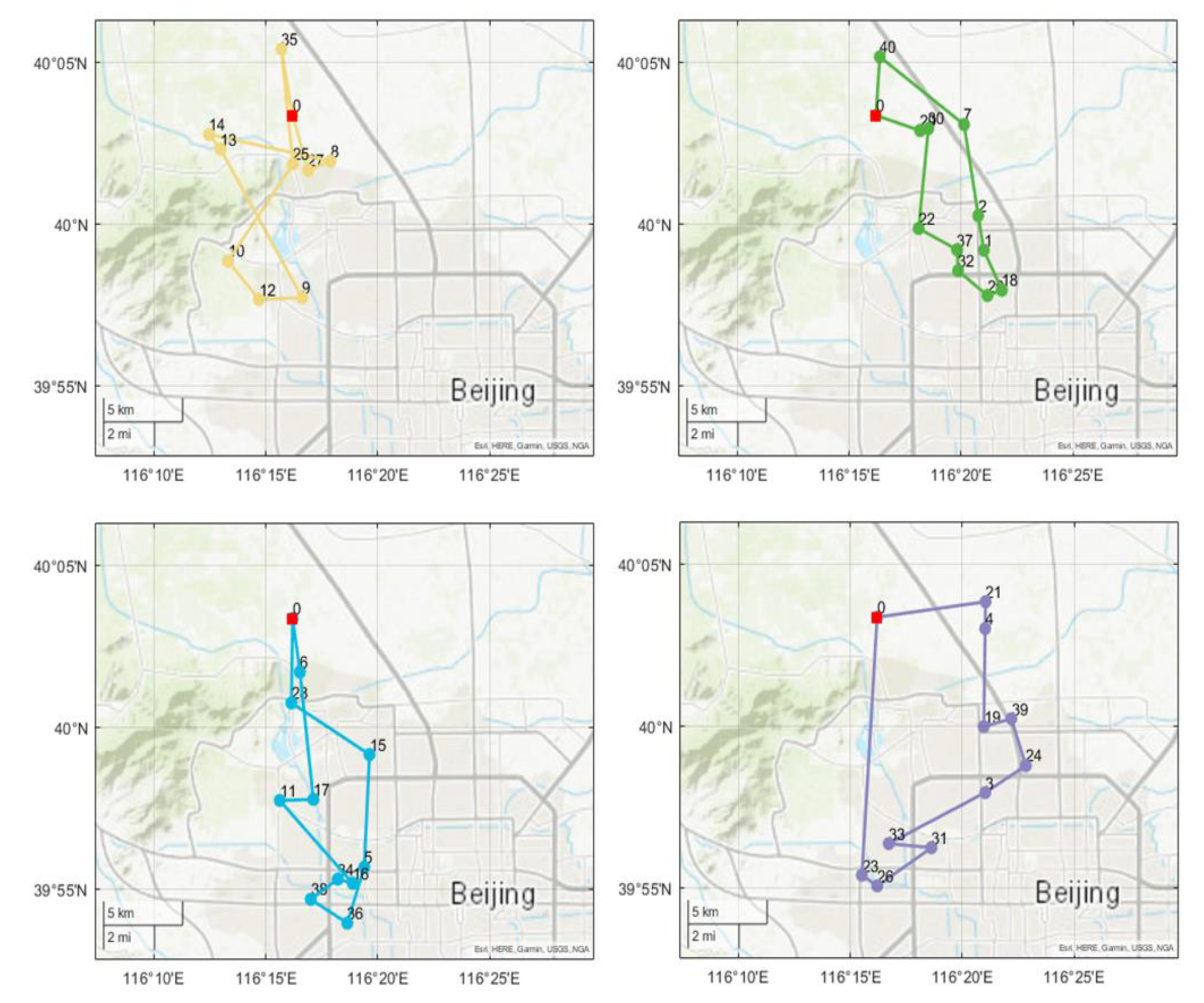
Sum		225.38	139.29	51.89	199.65	0.00	616.22

reports the best plan, and Figure 7 shows the routes on the map.

The results show that four trucks were employed to complete the day’s task. First, in terms of numerical analysis, the total cost for each truck did not exceed 200 RMB, with $C_t$ and $C_{r3}$ accounting for a larger share. All trucks traveled a total of 307.69 km and consumed 72.5 L of fuel, incurring transportation costs of 225.38 RMB and waiting and transportation refrigeration costs of 51.89 RMB. In our model, the service refrigeration cost varies with the inputs to the model. In this case, this cost accounts for a total of 32.40%, implying that logistics companies should improve service efficiency and shorten service time to save costs. We find that the penalty cost is 0, indicating that the working hours of the drivers of each route do not exceed the specified limit. Second, in terms of the quality of the routes, the vehicles depart from the distribution center and return to the distribution center after serving the customers. The number of customers served by each vehicle is close, and the number of kilometers traveled is close, i.e., the driver’s workload is roughly equal. The majority of the trucks (2, 3, and 4) on each route did not fold back while meeting the time window (route 1 produced some degree of folding back to meet the time window for certain customers). The next subsections analyze the impact of each parameter of the model on the decision.

5.2.1. Impact of Seasonal Temperature

The seasonal temperature will significantly affect the refrigeration system usage frequency of the trucks, which is obviously higher in summer and lower in winter. The difference in ambient temperature will lead to a change in the parameters $T_{cool}$ and $\kappa$. The values of $T_{cool}$ for spring or autumn, summer and winter are 1, 1.25, and 0.75 h, respectively, and the values of $\kappa$ are 0.3, 0.4, and 0.2.

Table 5. Cost variation with the season (unit: RMB).

Season	${\mathit{C}}_{\mathit{t}}$	${\mathit{C}}_{\mathit{r}1}$	${\mathit{C}}_{\mathit{r}2}$	${\mathit{C}}_{\mathit{r}3}$	${\mathit{C}}_{\mathit{p}}$	Total
Spring/Autumn	224.53	111.43	39.40	199.65	0.00	575.02
Summer	225.38	139.29	51.89	199.65	0.00	616.22
Winter	225.38	83.58	25.95	199.65	0.00	534.56

shows the effect of temperature on various costs in different seasons. With the change of seasons, the highest cost of distribution was observed in summer and the lowest in winter. Two of the costs, $C_{r1}$ and $C_{r2}$, are most affected by temperature. Compared to the total cost in winter, the cost in spring and summer increased by 7.6% and 15.3%, respectively. In addition, the fuel consumption in spring or autumn, summer, and winter is 67.65, 72.50, and 62.89 L, respectively. This implies that improving the airtightness of vehicles and reducing the value of $\kappa$ in summer or avoiding exposure to the sunlight when parking may be ways to reduce pre-cooling costs and fuel consumption.

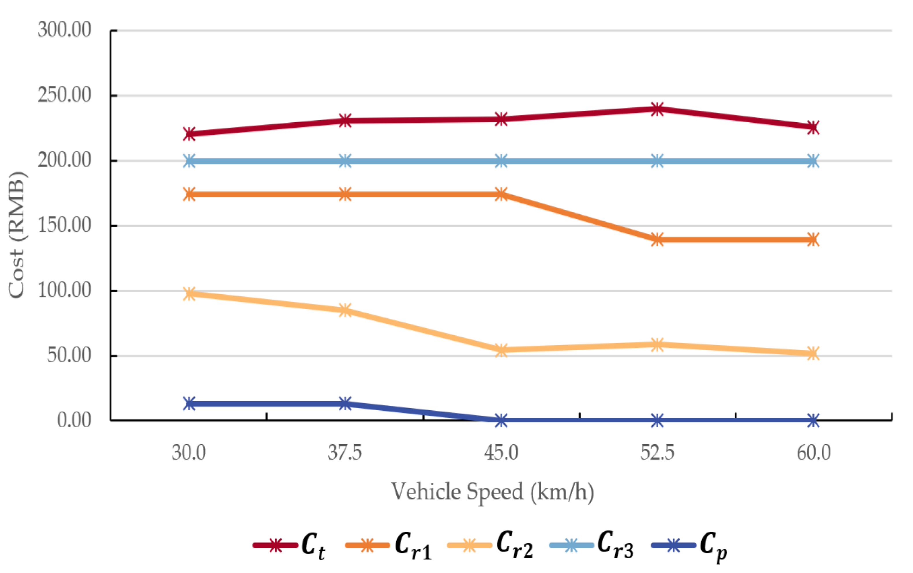
5.2.2. Impact of Vehicle Speed

In our model, we omit the effect of varied speeds on fuel consumption. However, the vehicle speed is an important influence in route planning, as it determines whether a vehicle can serve a given customer at a given time, affects the magnitude of $C_{r2}$, and influences the tradeoff between the costs. Figure 8 shows the tradeoff curves for the costs incurred for average speeds $v$ of 30.0, 37.5, 45.0, 52.5, and 60.0 km/h, respectively.

Overall, the total cost of the system decreases as the average speed $v$ increases. However, $C_t$ increases and then decreases as the parameter $v$ increases. The reason for this phenomenon is the change in the number of trucks employed. When $v$ is less than or equal to 45 km/h, five trucks are used to increase the pre-cooling cost while decreasing the $C_{r2}$. When the vehicle speed increases to 52.5 km/h, the decrease in the number of vehicles used leads to a decrease in the pre-cooling cost but increases the $C_{r2}$. We are surprised to find that when $v=60$km/h, the number of vehicles decreases to the minimum (derived from the ratio of total demand to total capacity) while $C_t$ and $C_{r2}$ decrease, and the $C_p$ is zero.

In reality, the speed of the vehicle depends on external factors such as the road conditions of the day, whether it is a working day or not. These external factors will affect the outcome of the decision. Predicting vehicle speed helps decision-makers to specify more reasonable planning. Especially when the average speed variation of vehicles decreases, it not only incurs penalty costs but also increases the number of hired drivers. Although our model does not consider the cost of drivers, adding more vehicles may lead to additional overhead and reduce the load rates of the vehicles.

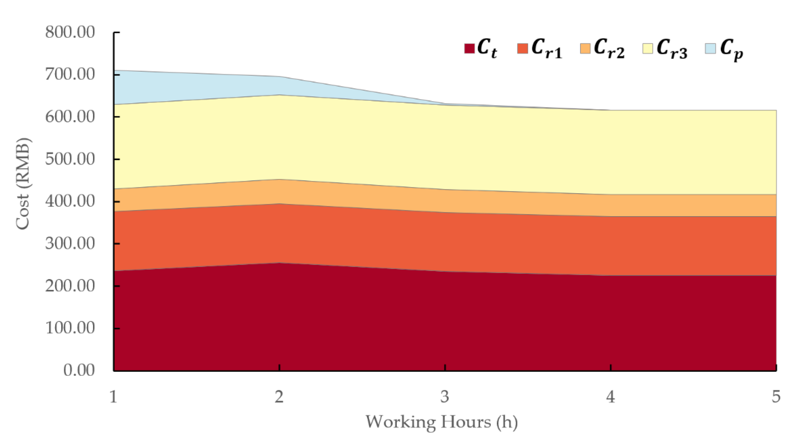
5.2.3. Impact of Driver Working Hours

In this subsection, we analyze the impact of parameter $T_{lim}$ on total costs. We want to know the impact of shorter working hours on fuel consumption. As mentioned earlier, the penalty cost is reflected in the cost of potential accidents and the additional wages incurred for working more than the $T_{lim}$. Figure 9 reports the trend and trade-off curves for the change in costs as $T_{lim}$ varies. We find that as $T_{lim}$ increases, the total cost gradually decreases by 13.24%. When $T_{lim}$ equals 3, the penalty cost incurred is equal to 3.26 RMB, and when $T_{lim}$ is greater than 3, the system does not incur a penalty cost, indicating that the work can be completed in close to 3 h per vehicle, satisfying the road safety law that drivers should not drive for more than four consecutive hours.

We also find that the system incurs penalty costs when $T_{lim}$ is equal to 1 or 2. In order to reduce the penalty cost, the transportation cost increases accordingly. This indicates that the quality of the route may deteriorate further to complete the task as soon as possible.

In this case study, the transport volume was not very large, and all vehicles completed their tasks in close to three hours. The above analysis shows that the parameter $T_{lim}$ will significantly affect the cost and the quality of the route. In real life, it is difficult to describe the penalty cost mathematically. In most cases, the driver delivers the vaccine safely to the customer at the specified time, incurring almost no penalty cost. However, the small probability of an accident generating damage would be difficult to bear. The more realistic implication of analyzing the impact of $T_{lim}$ is to equalize the workload of individual drivers.

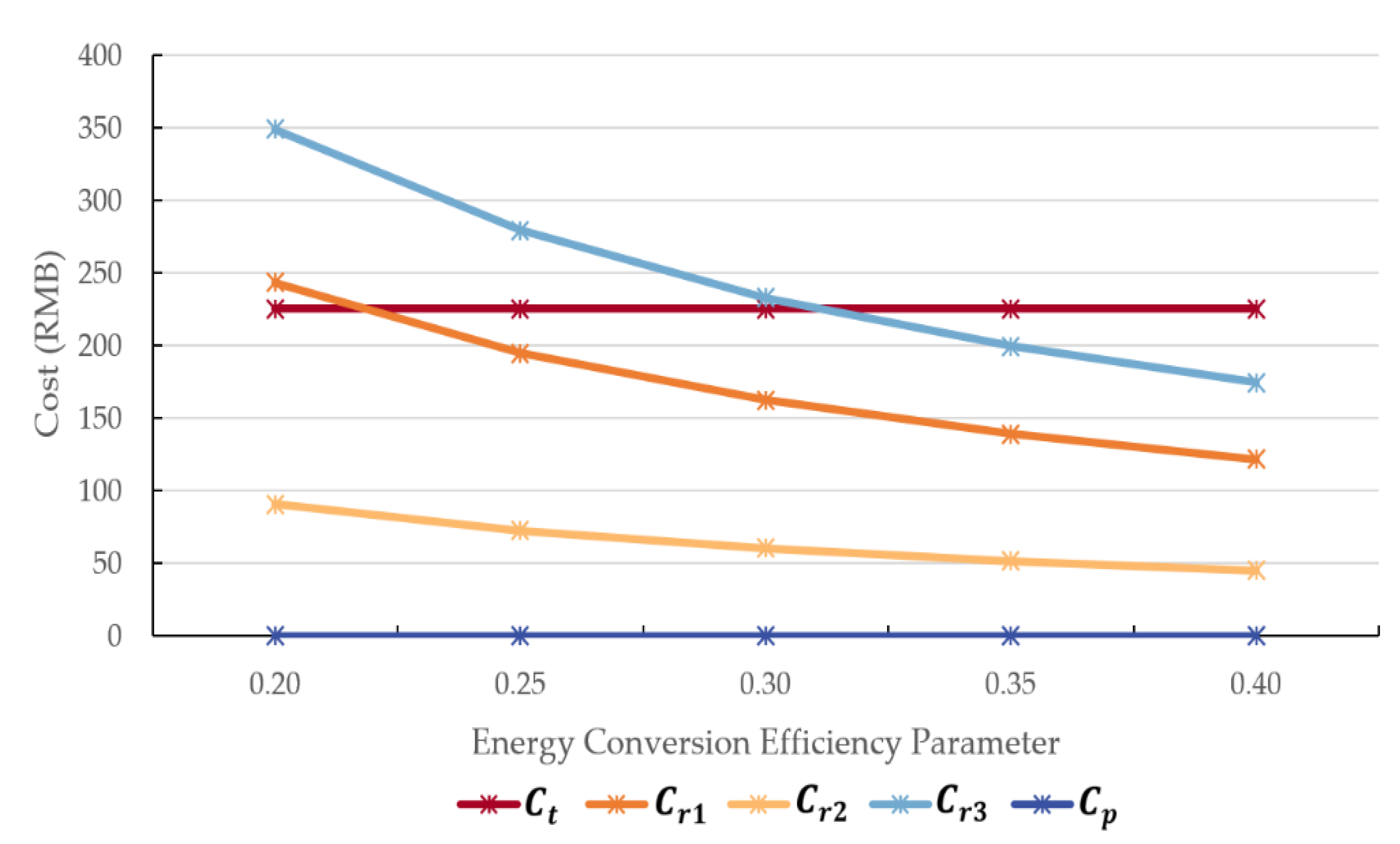
5.2.4. Impact of Energy Conversion Efficiency

The parameter $\eta$ indicates the conversion efficiency of the two energies, and the value is closely related to the parameters of the vehicle engine and the refrigeration system. The value of $\eta$ can be increased by replacing it with more advanced refrigeration equipment. Assuming that $\eta$ can vary between 0.2 and 0.4, the impact of this parameter on the cost is analyzed in Figure 10.

Provided that other parameters remain unchanged in Section 5.2, we find that the values of transportation cost and penalty cost are constant, indicating that a variation of this parameter does not affect route planning but significantly affects fuel consumption. Since the refrigeration cost is negatively proportional to this parameter, when $\eta$ is small, a small increase in variation of $\eta$ will reduce fuel consumption significantly. When $\eta$ is equal to 0.2, 0.3, and 0.4, the fuel consumption is 107.0, 80.2, and 66.7 L, respectively. Assuming that the current equipment is updated, and the parameter $\eta$ of the new equipment is equal to 0.4, then this distribution mission will save 6.2 L of fuel, which is 8.56% less than the fuel consumption with the old. Therefore, the logistics enterprise should weigh the cost of investing in new equipment and environmental protection and make a choice about updating advanced refrigeration equipment with full consideration of long-term economic benefits and the enterprise’s environmental responsibility.

6. Conclusions

This paper investigates a vehicle routing problem for vaccine distribution considering fuel consumption. The fuel consumption in each operation step is converted into the fuel cost. We propose a GA-LNS with the TSP-split metaheuristic method. Solutions to Solomon R1, C1, and RC1 benchmark show that the algorithm can solve a realistic scale problem. The result of a case study suggests that 60% of the fuel consumption in vaccine distribution comes from the refrigeration system. Moreover, fuel consumption is 15.3% higher in summer than that in winter, and reducing working hours does not have a large impact on fuel consumption.

Our findings also raise new questions for future research. First, in the present model, an idealized assumption is made about the relationship between fuel consumption and transport distance. As we mentioned, complex road conditions, driving habits, etc., can affect fuel consumption. By analogy, we can refine the fuel consumption more in each step of vaccine distribution, including factors such as the sealing of the carriage can be taken into account. Secondly, the content of our study is the traditional vehicle. The emergence of refrigerated electric trucks will generate more considerations in the model, including the rational allocation of power to the compartment cooling and driving the vehicle. This will be an interesting topic.