Management Soil Zones, Irrigation, and Fertigation Effects on Yield and Oil Content of Coriandrum sativum L. Using Precision Agriculture with Fuzzy k-Means Clustering

Abstract

Precision agriculture (PA), management zone (MZ) strategies at the field level, soil analyses, deficit irrigation (DI), and fertilizer Variable Rate Application (VRA) are management strategies that help farmers improve crop production, fertilizer use efficiency, and irrigation water use efficiency (IWUE). In order to further investigate these management strategies, the effects of four soil MZ treatments, which were delineated using PA with fuzzy k-means clustering, two irrigation levels [IR1:FI = full drip irrigation (>90% of ${\theta }_{fc}$), IR2:VDI = variable deficit drip irrigation (60–75% of ${\theta }_{fc}$)], and four VRA fertilizations were studied on coriander yield and essential oil content in a two-year research project in Greece. A daily soil-water-crop-atmosphere (SWCA) balance model and a daily depletion model were developed using sensor measurements (climatic parameter sensors as well as soil moisture sensors). Unbalanced one-way ANOVA (p = 0.05) statistical analysis results revealed that correct delineation of MZs by PA with fuzzy k-means clustering, if applied under deficit irrigation and VRA fertilization, leads to increased essential oil content of coriander with statistically significant differences (SSD) and lower fruit yields; however, without SSD differences among management zones, when appropriate VRA fertilization is applied to leverage soil nutrient levels through the different fuzzy clustered MZs for farming sustainability. Moreover, VDI compared to full irrigation in different MZs yields 22.85% to 29.44% in water savings, thus raising IWUE (up to 64.112 kg m⁻³), nitrogen efficiency (up to 5.623), and N-P-K fertilizer productivity (up to 5.329).

1. Introduction

Approximately 70% of our planet’s area is occupied by water [1,2,3]; however, just 2.5% is fresh water [4]. The Earth’s most confined freshwater resources are valued at 35,000,000 km². Low proportions of these fresh water supplies are directly accessible to mankind in river bodies, reachable lakes, groundwater, soil moisture (SM), or precipitation [5]. Humanity is overusing confined freshwater resources [3], resulting in water scarcity that endangers several regions of the world, with approximately 800 million humans not having adequate access to portable water and 2,500,000 million lacking appropriate sanitation, indicating that the problem is expected to intensify in the coming years [6]. Agriculture is the biggest freshwater user on earth, absorbing almost two-thirds of overall withdrawals [3,7]. The agricultural segment represents 70% of the earth’s freshwater abstractions [3,8,9], 59% of overall freshwater usage in Europe (EU), and around 284,000 million m³ are pumped yearly in order to serve EU requirements [10]. Presently, a lot of nations across the world are confronted with a shortage of fresh water [3,6,7,8,9,10,11] for drinking and irrigational purposes. The planet’s water requirements are foreseen to grow by 55% over the period 2000–2050, from 3500 to 5425 km³. Data analysis has revealed that climate change will have detrimental consequences for the earth’s water supplies, food productivity, and yields, resulting in a high extent of inter-regional variation and deficit [12,13,14]. This situation is predicted to escalate the pressures on the world’s existing freshwater reserves, with a concurrent growth of 70–90% in irrigation water demands by 2050 [15,16]. The quantity of irrigation water has consistently been the principal driver constraining plant yields in the world’s majority, where precipitation is inadequate to match plant water demands [3,9,14]. Global cropping productivity has considerably risen in the last century, boosting the irrigated land by a factor of almost six and raising the pressure on the irrigation water requirements [14]. The frantic rising and growing demand for the world’s diminishing water reserves and the continuously escalating consumption of agricultural products, the challenge of enhancing the effectiveness and capacity of irrigation water consumption by crops, guaranteeing the future security of food and crop commodities, and addressing the ambiguities arising from climate change have never seemed so critical [17].

A promising way forward to relieve the growing worldwide water shortage could be to exploit existing irrigation water supplies (precipitation, surface and subsurface water, and effluents) in a more viable, wise, and eco-friendly manner [18]. The above objectives could be accomplished by optimizing farm, soil, irrigation, and crop zone management.

In the coming decades, the world will be faced with the challenge of boosting crop yields using less water [18]. Precision agriculture (PA) and deficit irrigation (DI) are agricultural and irrigational management practices that assist growers in increasing the yield of their crops and optimizing water effectiveness and capacity, soilbed, farm supplies, and other inputs (pesticides, grains, manures, chemical fertilization products, etc.).

The PA industry is projected to increase from € 8.1 billion in 2022 to € 14.8 billion by 2030 as a result of the increasing acceptance of technologies such as auto-steering, positioning systems, remote sensing, various sensoring devices, GIS, agrodrones, PA computer programs, smart phone apps, and VRA applications [18]. The DI is an irrigation strategy that implements less water than the quantity used for complete watering. VDI is recognized as a core component as it helps to enhance irrigation IWUEs [3,18,19,20,21]. The consequences of DI on plant productivity, water uptake, and IWUE were investigated for many agricultural plants, legumes, vegetables, herbs, and spices [14,18,19,20,21,22,23,24,25,26,27,28].

Aromatic plant and spice sectors have been undergoing rapid expansion for many decades due to rising consumption in developing economies in conjunction with their rising importance for health and gastronomic benefits [14,29]. The global herb and spice market with miscellaneous products nowadays represents a multi-billion-dollar industry that is thriving thanks to global sales and the spread of production areas [29]. An extremely valuable aromatic herb-spice is coriander (Coriandrum sativum L.), or cilantro. It is a member of the Apiaceae (Umbellifera) family, which is recognized as an indigenous plant to Mediterranean countries, Western Europe, and Asia. This herb has been utilized since the ancient ages for cooking, pharmaceutical treatment, and perfumery [14,30,31,32,33,34,35]. The essential oil that is being extracted from the coriander berries (usually called seeds) has multiple usages [14,30,31,32,33,34,35,36] and it is normally removed from the fruits, generally either by steam distillation, hydro-distillation, or the new microwave-assisted hydrodistillation methodology [37]. The essential oil content was reported to range from 0.125 to 1.90% (v·w⁻¹), including 60–70% of linalool, the substance that produces the pleasant, distinctive aroma [14,30,32,33,36,37,38,39,40,41,42,43,44]. It is noteworthy that out of 60 essential oil crops, coriander herb had the largest yearly harvest (710 tons) and the greatest market value (USD 49.7 million) among 21 of the 60 crops [31]. The cilantro has numerous healing effects, such as anti-inflammatory, analgesic, antispasmodic, blood pressure reducer, high cholesterol reducer, anti-oxidant, anti-diabetic, anti-metabolic, calming-sleeping, protector against lead poisoning, and heavy metal detoxicant [14,32,45]. The presence of soil moisture (SM) is regarded as vital for the recycling of nutrients, a precondition for prime plant growth [3] so the hydraulic parameters of the soil that affect water movement, infiltration, and SM retention are regarded as key components to plant growth and should be considered as important factors in management zone delineation. In addition, SM influences evapotranspiration, which is a fundamental mechanism in the climatic cycle and a link between the water, energy, and carbon chains [9,11,14,17,18,46,47,48], and also influences a range of different procedures associated with crop growth and agro-food production, including a number of soil functions [3,17,48,49,50,51,52].

Precipitation and irrigation provide SM, and they are utilized for crop yields; however, moisture would be depleted more and more in mid-latitudes as a result of climatic and land usage alterations [51]. As is obvious, limited water reserves often constrain plant yields in semi-arid soils. Water resources decline and shortages due to many environmental impacts and overuse of irrigation systems are significant environmental concerns around the world [11,20,47]. In terms of new agricultural practices, PA refers to a managerial strategy that collects datasets utilizing a variety of modes, tools, and procedures, parses them in time, space, and single geodata, and synthesizes them with various other digital or analog inputs to support appropriate crop farming decisions based on assessed field diversity to improve resource utilization efficiently, improve yields, quality, profitability, and sustainability [14,18]. On the contrary, the conventional practice employs the entire-field management method, in which every farmfield is managed as a homogeneous crop area (but in reality, it is not) and does not take into account the variability of soil hydraulic, chemical, and granular parameters, the field’s topography, land use practices, or local prevailing climatic conditions. The various field inputs (irrigational water or wastewater, agrichemicals, fertilizers, etc.) are evenly spread over the entire field. This method is considered appealing to farmers for being quite fast and simple to operate, yet it leads to poor input efficiency, increased cultivation costs, and various inherent environmental costs. In addition, inadequate irrigational water and fertilizer application negatively affect crop growth and, consequently, yield. Regarding management zones, using classification algorithms [53,54,55,56,57,58,59,60,61,62,63,64,65,66,67] is considered an appropriate counterpart to correlation and regression. Soil data may be classified together or apart from additional data, such as spectral or yield, to “cluster” these data into feasible MZs. Towards this goal, grouping methods are widely adopted in PA, especially the fuzzy k-means algorithms and their variations [53,54,55,56,57,58,59,60,61,63,64,65,66], which create classes (MZs) with much better homogeneous performance in each MZ that can be considered functional management zones [63,64,65,66,67].

The two-year research aim was to study the effects of homogeneous management zones properly delineated using PA with fuzzy k-means clustering, variable deficit irrigation, and VRA fertilization on coriander fruit and essential oil yields.

2. Materials and Methods

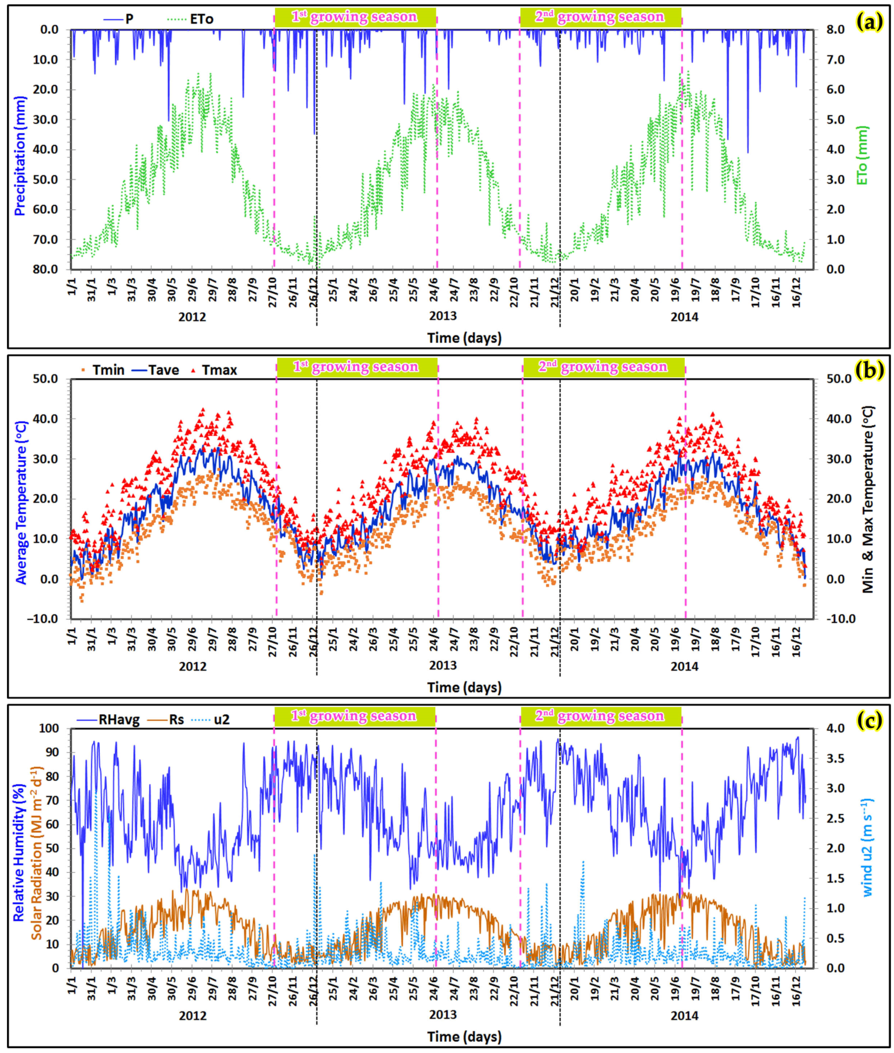
2.1. Study Area and Climatic Conditions

The two-year trial was undertaken on a farm located in the municipal unit of Krannonas (39°33′54.0″ N and 22°21′48.4″ E) of the Kileler Municipality, in the valley “Thessaly” in the Central Greece region. The climatic data were obtained from the local weather station. The area studied is dominated by a standard Mediterranean climate with a mild autumn with medium to high precipitation, a cold winter with high precipitation, a mild spring with low to medium precipitation, and a hot and dry summer with frequent hot temperatures and poor rainfall [3,9,11,14,21]. In the recent 10-year period, the mean annual rainfall was measured with sensors to an amount of 456.91 mm, the mean air temperature (AT) was 17.36 °C, the average maximum AT was 30.10 °C, the maximum AT was 45.50 °C, the average minimum AT was 7.39 °C, and the minimum AT was −12.70 °C. The average daily climate data for the 3-year climatic analysis, which is two growing seasons (g.s.) are depicted in Figure 1. Temperatures during the 2 g.s. varied as follows: average AT was 14.20 °C (±6.74), average maximum air temperature was 19.81 °C (±7.99), maximum AT was 40.20 °C, average minimum AT was 9.47 °C (±5.97), and minimum AT was −3.70 °C.

A careful reading of climatic variables shows that air temperature (average, higher, and lower), relative humidity, and wind speed have permissible values that are suitable for the appropriate development of the coriander plant. In contrast, the volume of precipitation and its timing in the four growth stages of the coriander (November to June) do not adequately meet the crop’s water demand; therefore, irrigation is necessary to achieve good yields. Indeed, the cumulative precipitation that fell throughout the coriander’s growing season was recorded as a mean precipitation of 290.90 mm, and it was found to be 360.20 mm and 221.60 mm in the 1st and 2nd growing seasons, respectively. The evapotranspiration of the crop (computed using the Penman-Monteith methodology [3,18,19,23,28]) in the various MZs of the field was found to be between 558.77 and 564.44 mm in the 1st g.s., whereas in the 2nd g.s. was found to be between 519.43 and 521.97 mm. The aforementioned data on the local climate are crucial because they have a direct impact on crop growth, evapotranspiration, and plant water demands. However, apart from air temperature and precipitation, there are a number of other climate parameters that affect the water demand of crops. The most influential parameters are the air’s relative humidity, wind speed, and solar radiation.

2.2. Experimental Design and Variants

The coriander’s experimental design was a four management soil zones unbalanced design since the four MZs were the de facto treatments (MZx where x = 1…4) (

Table 1. Experimental variants (factors and levels) in 1st and 2nd cultivation season.

Trial Season	Factors
1st cultivation season	1st MZ		2nd MZ		3rd MZ		4th MZ
Percentage of field’s cultivated area	23.61%		24.31%		23.61%		28.47%
Irrigation levels	IR1:FI *	IR2:VDI **	IR1:FI *	IR2:VDI **	IR1:FI *	IR2:VDI **	IR1:FI *	IR2:VDI **
VRA mean Nitrogen levels (kg·ha−1)	518.985	518.985	593.528	593.528	548.310	548.310	572.270	572.270
VRA mean P2O5 levels (kg·ha−1)	28.648	28.648	45.290	45.290	49.929	49.929	25.168	25.168
2nd cultivation season	1st MZ		2nd MZ		3rd MZ		4th MZ
Irrigation levels	IR1:FI *	IR2:VDI **	IR1:FI *	IR2:VDI **	IR1:FI *	IR2:VDI **	IR1:FI *	IR2:VDI **
VRA mean Nitrogen levels (kg·ha−1)	612.402	612.402	611.334	611.334	594.916	594.916	595.160	595.160
VRA mean P2O5 levels (kg·ha−1)	44.404	44.404	40.761	40.761	39.943	39.943	44.799	44.799

(*) IR1:FI = Full Irrigation (>90% of ${\theta }_{fc}$), (**) IR2:VDI = Variable Deficit Irrigation (60–75% of ${\theta }_{fc}$).

) obtained by PA with a fuzzy k-means clustering algorithm. Moreover, every MZ had two irrigation levels [MZx-IR1: full irrigation (>90% of ${\theta }_{fc}$) where x = 1…4, MZx-IR2: variable deficit irrigation (60–75% of ${\theta }_{fc}$) where x = 1…4, using a surface drip irrigation system].

Additionally, nitrogen and phosphorous P-Olsen VRA (Variable Rate Application) fertilization were applied in MZs. In the 1st and 2nd cultivation seasons (c.s.), VRA fertilizations of N-P-K = (518.985 to 593.528)-(25.168 to 49.929)-(0) kg·ha⁻¹ and N-P-K = (594.916–612.402)-(39.943–44.799)-(0) kg·ha⁻¹ were applied, respectively. The field’s overall cultivated area was 546.72 m², which was divided into 48 irrigational trial plot units with dimensions of 1.70 m width × 6.70 m length (11.39 m²). Moreover, the field was divided into 144 sampling sub-plot units with dimensions of 1.70 m width × 2.23 m length (3.80 m²).

2.3. Crop, Cultivation Technology and Field Management

Crop: The Cilantro (Coriandrum sativum var. microcarpum L.) variety seeds were used. The cilantro herb is a tender, glabrous plant with varied-shaped leaves, widely oblique at the bottom of the stem and thin and winged higher up on the flower stalks.

The florets are produced in little umbrellas (umbels), which are white or light pink and asymmetric, with the petals directed away from the center of the umbrella (5–6 mm in length) than those directed towards it (1–3 mm in length). The fruit is a spherical, xeric schizocarpium with a diameter of 1.5–3 mm. The optimum period for planting the cilantro is the latter week of October to the early week of November [14]. So, the seeding for both years took place on the first week of November with the application of 20 kg·ha⁻¹ of Cilantro seeds at a distance of 40 cm between rows and 10 cm between plants.

Soil-Crop Management, Farm machines, Irrigation pipeline system: In both years, the field was plowed in early October with a four-row reversible mounted plow. A row of spring-steel tine cultivators (with inverting points and wheels with floating wings) was deployed into the field in late October. This particular kind of cultivator is engineered to cultivate the soil between crop rows, aerating the topsoil, uprooting, and destroying any existing weeds. In addition, the wheels with floating wings create a clear, neat, uniform, and stable finish on the seedbed for maximal seed germination and crop establishment.

The irrigation pipeline system was composed of a header module with (a) a hydrocyclone; (b) a screening water filter; (c) a fertigation device; (d) several fittings; (e) a master water supply pipeline; (f) a main pipeline with branch aluminum pipelines (Φ = 90 mm/16.21 bar); and (g) polyethylene drip lateral pipelines (Φ = 20 mm/3.8 L·h⁻¹/0.40 m) having integrated pressure compensation drippers. Prior to their use in the field trials, the drippers were thoroughly checked in the laboratory to guarantee their adequate functionality. The drippers had an outflow rate of 3.8 L·h⁻¹ at a test pressure of 253.31 kPa, in accordance with I.S.O. standards [68]. The watering system managed moisture after seeding, and favorable climatic factors (appropriate air and soil temperatures) in the subsequent days allowed the seeds to emerge with a population of 2304 plants per area unit⁻¹ (area unit = 11.39 m²) or 2,021,691 plants·ha⁻¹. No herbicides were applied to the crop; therefore, weed control was carried out by hand. Finally, in both cultivation years, the coriander plants were harvested in late June at the full maturity phase, when there were only brown-colored fruits.

2.4. Observations and Determinations

(a) Soil parameters and soil laboratory analysis: Effective coriander roots grow at 0–30 cm [14], at which point in a standard water extraction scheme the roots uptake approximately 90.00% moisture and the beneficial nutrients present in the soil-water solution. Thus, to define the soil’s chemical, physical, and hydraulic characteristics in the actual root zone (0.00–30.00 cm deep), systematic sampling was conducted in the 144 sampling sub-plot units. A GPS detector was employed to locate the geolocations of the 144 soil samples collected and then analyzed in the department’s applied soil science laboratory. The 144 samples were cleaned from root residues, air-dried, and sieved through a grid (2 mm) in order to define texture (sand, silt, and clay contents) [48,50,69] using the Bouyoucos hydrometer method [69]. Soil samples from the field, after laboratory analysis, were found to be Sandy Clay Loam (SCL) soil [50,69]. The soil and crop data for the analysis were collected in two cultivation seasons from the field’s cultivated area (0.055 ha).

Soil pH was assessed in a 1:2 soil/water solution using a glass H⁺ sensing (indicator) electrode paired with a reference electrode connected to a pH monitor metering device.

The organic matter (OM) was assayed with chemical oxidation of 1 mol·L⁻¹ K₂Cr₂O₇ and by residual reagent titration with 0.5 mol·L⁻¹ FeSO₄ [57,58,70]. Inorganic nitrogen soil content was retrieved with 0.5 mol L⁻¹ of CaCl₂ and assessed by means of distillation in the presence of MgO and Devarda alloy, correspondingly. Available phosphorus P (Olsen method) was retrieved with 0.5 mol L⁻¹ of NaHCO₃ and measured with spectroscopy [48].

The exchangeable forms of potassium K⁺ were extruded by 1 mol L⁻¹ of CH₃COONH₄ and quantified using a flame spectrophotometer. The exchangeable magnesium Mg⁺⁺ and calcium Ca⁺⁺ cations were obtained by displacement of those elements from the soil colloids with ammonium (NH₄) by shaking the soil sample with 1.0 N ammonium acetate (NH₄OAc) adjusted to pH 7.0 with ammonium hydroxide (NH₄OH) and determined by an atomic absorption spectrophotometer (AAS Spectroscopy Varian-Spectra-AA-10plus, Victoria, Australia) using a flame and air-acetylene mixture [48,49]. The calcium carbonate was determined with a Bernard calcium meter. The assay consisted of the quantification of the CO₂ liberated when the specimen was processed using 6N HCL. In a sealed unit, the amount of CO₃²⁻ is strictly proportional to the increasing volume that results from the liberation of CO₂ [49]. The θfc (field capacity) and θwp (wilting point) were both obtained with the ceramic porous plate process, with 0.33 Atm for θfc and 15 Atm for θwp [3]. Dry bulk soil density has been determined by weighting soil volumetric samples (taken with a 45 mm diameter hydraulic undisturbed soil core sampler), drying them at 105 °C (dry time = 48 h), and estimating the results in dry soil g·cm⁻³ (overall undisturbed soil bulk volumes).

(b) Crop productivity parameters: At the completion of every growth stage (Lini (seedling), Ldev (flowering), Lmid (fruiting), and Llate (ripening)), three typical cilantro plants from every plot were destructively picked, and their fruits, if any, were counted. Additionally, the date for all plots when plants went into every phenological growth stage was logged. Measurements of plant height and the plant’s umbel heights were obtained with a tape meter (accuracy = 1 mm). The weights of the cilantro fruits were measured with a digital balance to the nearest 0.01 g. Cilantro (Coriandrum sativum var. microcarpum L.) fruits were harvested in late June (maturation phase), when in the plantation there were only brown-colored fruits. The results of postharvest treatment showed that the average diameter of the fruits was Df < 3 mm, whereas the average mass of 1000 Cilantro fruits was 9.47 g.

Following the fruits’ air drying in a shaded spot (8–9% humidity) in the lab, a two-rotary roller grain mill was employed to smash the coriander’s fruits, which were then sieved through a 2.0 mm metal grid prior to distilling. The ethereal oil concentration was obtained using hydro-extraction and hydro-distillation of cilantro seeds by means of a Clevenger distillation apparatus. A mass of 12.5 g of dehydrated cilantro seeds was immersed in 250 mL of distilled water with a hydrodistillation time period of 105 min. The hydro-extraction process was replicated in 3 repetitions for each fruit sampling, and the ethereal oil concentration was quantified as the dried weight (DW) base of the cilantro seed material (ml·100 g⁻¹).

(c) Moisture Monitoring and Modelling: Soil moisture readings were taken daily using time domain reflectometry (TDR), a nonradioactive method that relies on directly measuring the soil’s dielectric constant and converting it into water volumetric content [3,18,25], and has been reported to be fast and robust, regardless of soil type, apart from exceptional cases [20,71,72,73]. The TDR has been employed since it provides accurate readings with a margin error of ±1% [18,19,20,25,72,73]. a TDR device and probes engineered in five sensors each at depths of 0–15, 15–30, 30–45, 45–60, and 60–75 cm [18,19,20,21,25] that were deployed for measuring soil water content (θvi, …, θvn) with i = 1, 2, …, n, and n = 5, of the cilantro root area for n soil layers. SM-data readings have been entered daily into a geodatabase using PA for modeling, and they were also integrated into the SWCA model, and the mean daily θv_(TDR) has been assessed by means of interpolating the day-to-day SM records at several depths assigned to the various soil layers according to [18].

(d) Net Irrigation Requirements, Evapotranspiration, Soil–Water–Crop–Atmosphere (SWCA) Model, Soil Moisture Depletion Model: Day-to-day climate inputs (air temperature, relative humidity, atmospheric pressure, wind force, precipitation, and solar radiation) were acquired from sensor readings from a weather station located near the field. Net irrigation requirements (NIR) were computed by applying a daily SWCA (soil-water-crop-atmosphere) model [17,18,25]. The reference evapotranspiration ETo was calculated according to the F.A.O. Penman-Monteith methodology [3,17,18]. The crop evapotranspiration (ETc) and the actual crop evapotranspiration (ETa) were computed according to [14,17,18] and based on crop coefficients derived from field readings of vegetation growth and index [17,18,25]. The effect of water stress on the crop transpiration coefficient (K_s) was assessed according to [18]. The value of the Kcb coefficient was adjusted for local climate and prevailing conditions [17,18]. The exhaustion of SM in the root zone was assessed by applying a daily Available Soil Moisture Depletion model (ASMD) [17,18,25] at the MZs scale.

(e) Fertilizer’s use productivity, and irrigation water use efficiency (IWUE): The fertilizer’s nitrogen partial factor productivity (N_pfp) was calculated according to [18,25,74,75]. The N-P-K (Nitrogen–Phosphorus–Potassium) fertilizer’s partial factor (pf) productivity (NPK_pfp) was calculated according to [18]. The Irrigation Water Use Efficiency (IWUE) [kg m⁻³], was estimated according to [18].

2.5. Data Preparation, Exploratory Geostatistics Analysis-Modelling, Interpolation, and Models Validation Measures

The sampled, measured, and analyzed lab soil data were digitized, modeled, geo-mapped in a GIS environment, and stored in a digital geodatabase according to the samples’ locations and attributes. To obtain the several GIS soil parameter variability maps of the field (20 parametric maps), spatial interpolation was applied using several OKr geostatistical models in order to assess an approximate estimate of the unknown location rate based on the observed values using exploratory geospatial analyses, geostatistical analysis, and modeling. The existence of a univariate pattern of normality can be verified graphically with the use of normal QQ plots and boxplots and numerically with the use of skewness and kurtosis statistic measures [76,77,78]. After normalizing the distribution of data points, several semivariogram models were tested and evaluated from a library of mathematical models featuring spatial relationships in geostatistical modeling. For the interpretation of spatial soil variation, semivariogram analysis and interpolation methods are mainly used. The kriging methodology is built on the presumptions that parameters’ attribute rates (soil’s chemical, granular, and hydraulic parameters; cilantro’s yields and ethereal oil concentrations; pf nitrogen fertilizer productivity; pf N-P-K fertilizer productivity; and IWUE of MZs) in the non-sampled areas are a well-weighted mean of the values in the sampled areas.

Furthermore, the validity of the outputs of geostatistical models necessitates statistical analyses of residual errors, the differences that exist within the forecasted and the observable values, and the classification of the forecast among overestimates and underestimates as outlined by previous studies [3,9,18,20,21,25,76,77,78,79,80,81,82]. These statistical metrics are the MPE (mean prediction error), the RMSE (root-mean-square error), the RRMSE (relative root mean square error) as a metric of prediction accuracy between parameters with different formats, the MSPE (mean standardized prediction error) as a metric of unbiased forecasts, the RMSSE (root-mean-square standardized error) as a benchmark for a proper assessment of the forecast variability [9,76,77,78,79,80,81,82], and the ASE (average standard error) as a measure of the accuracy of the true population mean [3]. MSPE and RMSSE metrics are employed to evaluate unbiasedness and uncertainty accordingly. MPE and MSPE metrics should approximate zero values for an optimum forecast; RMSSE should be close to 1, the lower the RMSE value, the better for an optimum forecast; the lower the RRMSE, the higher the accuracy; and a lower ASE indicates higher accuracy of the model.

2.6. Factor and PCA Analysis, Delineation of Management Zones with Fuzzy k-Means Clustering

In multivariate statistics, factor analysis is a powerful explanatory mechanism that can be employed to uncover and explain relationships between interacting parameters [3,9,76,80]. In our case, first multivariate factor analysis and then rotated (R-mode) factor analysis [9,76,80,81,82,83,84,85] were performed to extract the factors (components) governing the soil’s chemical, granular, and hydraulic parameters in the field. The extraction method used was the PCA [76,80,81,82,83,84,85,86] and the rotation method was the varimax method with Kaiser Normalization [3,9,76,84,85] by utilizing the measured and analyzed lab data (soil’s chemical, granular, and hydraulic parameters) on GIS parametric maps in order to extract the components (MZs). PCA analysis was conducted to group the data sets of soil chemical, granular, and hydraulic parameters into statistical components and generate linear independent variables that eliminate multicollinearity and provide a description of the spatio-temporal information obtained. The field’s MZs optimal number was obtained based on factor and PCA R-mode analyses of the various soil parameters, eigenvalue diagrams, 3-D and 2-D component diagrams in rotated space, and the realistic potential of MZs application in the trial pattern. Then, Fuzzy k-means clustering [51,52,53,54,55,56,57,58,59,60,61,62,63,64,65] was performed with the FuzME 3.5c software [62] and the Management Zone Analyst (MZA) 1.01 software [63] in order to cluster the soil parametric data into potential factors (MZs).

Firstly, grouping was carried out with the soil’s chemical parameter data (“soil chemical group”), then with the soil’s granular data (“soil granular group”), then with the soil’s hydraulic data (“soil hydraulic group"), and finally with all the soil data. An exploratory Fuzzy k-means clustering [53,54,55,56,57,58,59,60,61,62] analysis was conducted to clarify which distance metric, fuzziness exponent φ, and maximum iterations were best used with the available field soil data. Multiple runs of the software were performed in order to evaluate the results and select the final best distance metric, fuzziness exponents φ, and maximum iterations.

The final step was termed the “soil All parameters” group data and was regarded as the “reference” for MZs maps. The output MZ map of the “soil All parameters” (20 parameters) data clustering was compared with the generated MZ maps of “soil All parameters” with various fuzziness exponents. The “soil chemical group” map (8 parameters), the “soil granular group” map (6 parameters), and the “soil hydraulic group” map (6 soil’s hydraulic parameters) were compared with the generated MZ maps’ clustered outputs with various fuzziness exponents in order to determine the introduced fuzzy metric of the Percentage of Management Zones Spatial Agreement (PoMZSA) (%) between the reference (All parameters) map and the rest of the MZ output goal (target) maps, i.e., the percentage of map cells that belong to the same clade in the reference map and the goal maps. This method gives a percentage approximation of the spatial correlation of each MZ of the goal map with the corresponding zone of the reference (‘All parameters’) map, and the percentage of cells summarizing the agreement of each MZ and all the zones in the goal map gives a percentage approximation of the spatial correlation of the compared maps.

2.7. Statistical Analyses

The MZs of the field were the de facto “treatments”, and since they were not equal in magnitude, unbalanced one-way ANOVA statistical analysis was conducted using the statistics software IBM SPSS v.27 (IBM, Armonk, NY, USA). The outcomes reflect the averages of the sampled and measured data. The means were separated using the Tuckey and Games-Howell statistic tests as a control criterion when significantly different scores occurred (p = 0.05) between treatments [3,18,76]. The descriptive statistics were calculated [76,77,78,79,80], while ANOVA [3,9,78,79] was applied to examine how adequately the variability of fruit yield and essential oil is attributed to the various MZ soil maps.

3. Results

3.1. Results and Discussion of Soil’s Chemical, Granular and Hydraulic Analyses

The complete data analytics results as descriptive statistical measures are reported in

Table 2. Descriptive statistics of main soil chemical, granular, and hydraulic parameters of the 144 sampling sub-plot units.

SN	Parameter	Minimum	Maximum	Mean	Std. Deviation *	Variance	CV (%)	Range
1	Calcium Ca++ (mg·kg−1)	1190.84	3472.84	2236.16	427.38	182,653.09	19.11	2282.00
2	Calcium carbonate CaCO3 (%)	0.37	4.22	1.57	0.83	0.68	52.58	3.85
3	Magnesium Mg++ (mg·kg−1)	1100.82	2876.33	1900.58	304.55	92,753.40	16.02	1775.51
4	Nitrogen inorganic(mg·kg−1)	47.50	101.00	68.09	10.34	106.98	15.19	53.50
5	Organic matter (%)	1.33	4.07	1.79	0.33	0.11	18.49	2.74
6	pH [1:2 soil/water solution]	7.45	8.13	7.82	0.09	0.01	1.22	0.68
7	Phosphorus P-olsen (mg·kg−1)	8.96	21.43	15.95	2.29	5.24	14.35	12.47
8	Potassium K+ (mg·kg−1)	238.50	758.51	409.43	81.04	6566.86	19.79	520.01
9	Clay (size: <0.002 mm) (%)	22.18	28.72	24.83	1.13	1.28	4.55	6.54
10	Gravel (%)	0.01	0.25	0.08	0.03	0.00	43.66	0.23
11	Sand pr (size: 0.2–2 mm) (%)	30.13	35.69	33.37	1.32	1.74	3.95	5.57
12	Silt (size: 0.002–0.02 mm) (%)	13.61	22.31	19.66	1.69	2.87	8.61	8.70
13	Soil Erodibility [Kfactor] (Mg·ha·h·ha−1·MJ−1·mm−1)	0.02	0.03	0.03	0.00	0.00	4.73	0.01
14	Vfs sand (size: 0.02–0.2 mm) (%)	20.72	23.06	21.94	0.16	0.03	0.74	2.34
15	Bulk density (g·cm−1)	1.31	1.66	1.41	0.05	0.00	3.90	0.35
16	Field capacity θfc (m3·m−3)	25.12	30.47	27.66	0.92	0.85	3.34	5.34
17	Plant available water (cm·cm−1)	0.08	0.13	0.11	0.01	0.00	6.11	0.05
18	Saturation θsat (m3·m−3)	37.29	50.55	46.68	2.21	4.90	4.74	13.25
19	Sat. Hydraulic conductivity Ks (mm·h−1)	4.66	22.94	16.27	4.22	17.85	25.96	18.28
20	Wilting point θwp (m3·m−3)	13.36	17.97	15.98	0.67	0.45	4.20	4.61

* Std. Deviation or SD = standard deviation of the data points.

. The soil properties of the experimental field differed widely, and a closer examination of the outcome of the chemical, granular, and hydraulic analysis of the soil in the laboratory showed that the field’s soil was appropriate for the growth of coriander [14,17,48]. The calcium Ca⁺⁺ (mg·kg⁻¹), magnesium Mg⁺⁺ (mg·kg⁻¹), potassium K⁺ (mg·kg⁻¹), nitrogen inorganic (mg·kg⁻¹), saturation θsat (m³·m⁻³), sand pr (size: 0.2–2 mm) (%), and field capacity θfc (m³·m⁻³) presented high average values (≥27.66), while the other attributes had low average values (<27.66). Soil texture, which affects nearly any aspect of soil management and especially tillage, was classified as sandy clay loam (SCL) [17,48]. The mean calcium Ca⁺⁺ level was classified as high [3,48,50]. The mean calcium carbonate, CaCO₃, was classified as medium-level [3,48]. The mean magnesium Mg⁺⁺ in accordance with the clay percent content of the soil is considered a high Mg⁺⁺ level [3,48,50].

The majority of information on nitrogen fertility is addressed to agronomic crops. In principle, 112 to 336 mg·kg⁻¹ should be considered adequate for proper grass growth [50]. An oversupply of nitrogen causes a delay in ripening, triggers growth, increases insect infestations, and promotes diseases. The mean Nitrogen inorganic found in the field is characterized as a low to medium level of nitrogen [3,14]. An adequate amount for proper coriander growth would be 150 to 250 mg·kg⁻¹ [14]. It is necessary and environmentally friendly to implement nitrogen based on the needs of the crop in such a way as to minimize the residual soil nitrogen at the close of the growing season and ensure that there is minimal nitrogen left for losses. Therefore, it is significant to study the amount of nitrogen application that gives an economically viable yield without the negative side effects of scarcity. Thus, we chose VRA fertilization under full and deficit irrigation and statistically investigated the coriander yields of the different MZs results. The applied fertilizer VRA is a promising method in precision agriculture that can reduce nitrogen and other fertilizer amounts, decrease economic costs, and reduce nitrogen leaching.

Soil organic matter (OM) results were classified as low to high, with a mean that is classified as a moderate OM level [3,20,48] indicating average structural conditions and average structural stability in soil. These results could be attributed to the high temperatures that occurred in the spring and summer in this study area, the low vegetation cover, and probably to the lack of organic manure utilization. OM is broadly recognized as a fundamental element of soil fertility due to its significant contribution to the chemical, physical, and biological activities that occur throughout the growing stages and provide plants with a variety of nutrients. The mean pH at 1:2 soil-water extract was categorized as alkaline. The optimal pH rate for cilantro is 7.0 [14] and is regarded as a well-tolerated limit [3,14]. The mean phosphorus P-Olsen level was classified as moderate [3,14]. Regarding phosphorus in soil, there is limited mobility, and the risk of leaching phosphorus is not regarded as a concern [3,18,28,48]. In contrast, the root mobility of phosphorus is the primary constraint on uptake methods. Due to the low mobility of phosphorus, coriander’s root uptake is the primary uptake method, independently of the soil’s pH. The exchangeable potassium K⁺ reached high concentration levels. The mobilization of potassium in soils is at the intermediate level; however, it is not leached out because it has a positive charge (K⁺); therefore, it is attracted to the negatively charged colloids in the soil [3,14,48]. The coriander plant requires potassium at the fruit-filling growth stage; to be accessible at this time, the K⁺ should be in soil-water solution where the late-season root system is dormant.

The hydraulic conductivity of the soil is helpful for forecasting water runoff from precipitation, drainage of the soil’s root horizons, irrigation amounts, and deep drainage, which is contributing to salinity [3,87,88]. The saturated hydraulic conductivity results were classified as slow to moderate. The mean soil erodibility of the field was categorized as moderate based on the USLE (Universal Soil Loss Equation) [89,90,91,92]. It is remarked that the results for θfc and θwp obtained from the hydraulic analysis of the soil are within the normal limits given by Allen et al. [17]. Furthermore, Allen et al. [17] propose that the depth of the topsoil evaporation layer Ze (m) should be between 0.10 and 0.15 m. In the current project, a value of Ze = 0.10 m was selected in the computations. The standard deviations of the considered attributes varied widely (Table 2). A small SD indicates that the data values are close to the mean, whereas a big SD indicates that the data values are scattered over a wide spread, as in the case of calcium Ca⁺⁺ (mg·kg⁻¹), magnesium Mg⁺⁺ (mg·kg⁻¹), potassium K⁺ (mg·kg⁻¹), and nitrogen inorganic (mg·kg⁻¹). Soil property variability as a number is depicted by the coefficient of variation (CV), and it is categorized into three main classes [93]: (a) low CV (CV < 15%), (b) moderate CV (CV = 15–35%), and (c) high coefficient of variation (CV > 35%). The CV percentages revealed that the variability classification attributed 12 out of 20 examined soil properties as low class (CV < 15%). Anthropogenic and/or environmental drivers, such as farming management, soil texture, soil chemical, granular, and hydraulic properties, soil processes, and climate change effects, could potentially all be contributors to the moderate and high variability.

3.2. Results and Discussion of Exploratory Data Analysis

An exploratory data analysis was performed prior to geostatistical modeling. Two important statistical measures of the examined soil properties in the experimental plots are skewness and Kurtosis [94]. After evaluating the skewness and kurtosis scores, a similarly occurring outcome for both statistic measures indicated that 8 out of a total of 20 parametric datasets of soil chemical, granular, and hydraulic properties needed to be transformed in order to verify that their datapoints were normally spread and that the assumption of variance equality of the data values was satisfied [84,95]. Taking into consideration the above findings, these datasets were transformed using a logarithmic transformation [79,95]. The transformed parameters were bulk density (g·cm⁻¹), calcium Ca⁺⁺ (mg·kg⁻¹), gravel (%), magnesium Mg⁺⁺ (mg·kg⁻¹), nitrogen inorganic (mg·kg⁻¹), organic matter (%), potassium K⁺ (mg·kg⁻¹), and soil erodibility (Mg·ha·h·ha⁻¹·MJ⁻¹·mm⁻¹).

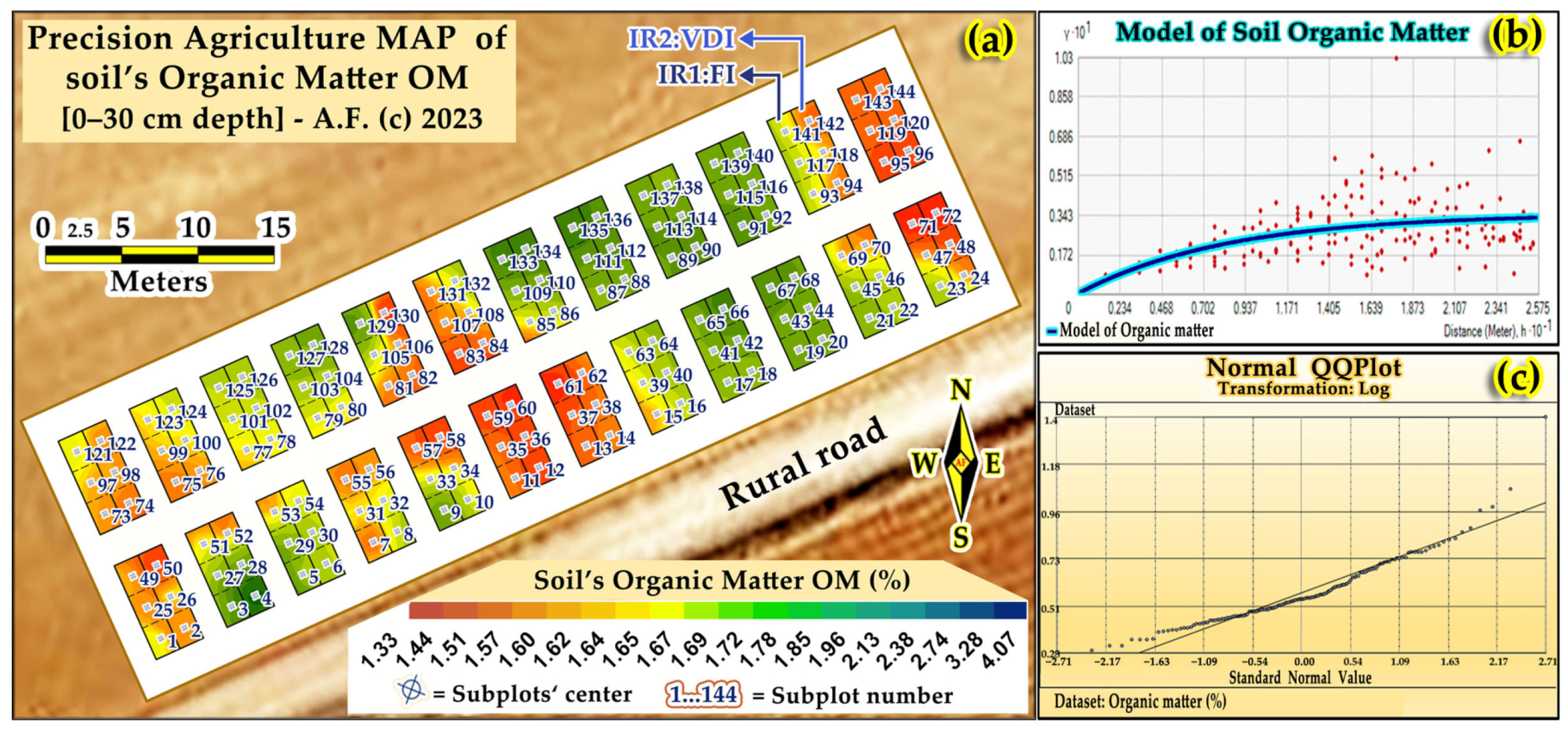
3.3. Results and Discussion of Precision Agriculture Geostatistical Modelling of Soil’s Chemical, Granular and Hydraulic Parameters

In agroecosystems, geostatistical analysis and modeling are important tools to assess the spatial variability of soil characteristics [3,18,20,21,25,87,88].

The most broadly applied interpolation model for predicting the spatial allocation pattern of soil, water, and crop features is the ordinary kriging (OKr) interpolation [3,18,20,21,70,76,95,96,97,98,99,100,101,102,103]. The choice of the Kriging model to be applied is dictated by the properties and statistical measures of the data and the preferred spatial model.

The field pattern with the sampling subplot units’ number (sn = 1…144) is depicted in a PA sampling subplot units map of OM (Figure 2a), along with the diagram of soil’s organic matter semivariogram model (Figure 2b) and the normal QQ Plot diagram of soil’s OM with Log transformation (Figure 2c). The Ordinary Kriging modeling method was used to predict the soil characteristic parameters for the non-sample areas [3,18,21,79,82,94,103,104,105] of the experimental field. This geostatistical method, due to its straightforwardness and precision [104], was employed in the present research.

The modeled PA spatial variability maps of the soil’s chemical, granular, and hydraulic parameters are depicted in the various final maps in Figure 3a–r. The created PA spatial variability maps of soil “Chemical Group” parameters revealed that calcium carbonate CaCO₃, inorganic nitrogen, and pH were similar in their spatial variability. Such consistent spatial variability occurs because those soil attributes are associated with each other and have high and moderate positive correlations. In addition, the southwestern and northeastern parts of the PA maps of pH (Figure 3b), nitrogen inorganic (Figure 3d), and calcium carbonate CaCO₃ (Figure 3h) showed the highest values of these parameters, while the central-northern and central-southern regions showed the lowest, plus the northern part in the case of CaCO₃. Likewise, the modeled PA maps revealed that organic matter (Figure 3a) and potassium K⁺ (Figure 3f) had matching spatial variability patterns throughout the field area because they are associated with each other with a high positive correlation. The PA map of soil magnesium Mg⁺⁺ (Figure 3c) presented an almost identical pattern (r = 0.953) of spatial variability with the calcium Ca⁺⁺ (Figure 3g), a relatively high similarity (r = 0.548) with CaCO₃ (Figure 3h), and a partly similar pH pattern. An agronomist can be greatly assisted in recognizing and locating field sites of low, medium, and high soil fertility by studying and analyzing precision agriculture’s spatial variability maps of soil “Chemical Group” parameters (Figure 3) and comprehending the effect of each parameter on crop growth.

The accurate prediction of these soil parameters is therefore driven by the presence of spatial dependence among the field’s sample observations, as estimated by the correlogram or semivariogram [104]. The various modeled spatial variability maps of soil’s “Hydraulic Group” parameters are depicted in Figure 3m–r. The generated map of saturation θsat (Figure 3o) depicted a highly congruent spatial variability pattern with the plant available water PAW (Figure 3r) map pattern (r = 0.867) and saturated hydraulic conductivity Ks (Figure 3p) map pattern (r = 0.825), whereas it presented a highly negative correlation (r = −0.991) similar pattern with the soil’s bulk density (Figure 3q).

The developed map of plant available water (Figure 3r) presented a highly congruent spatial variability pattern with θsat (Figure 3o) and saturated hydraulic conductivity Ks (Figure 3p) (r = 0.768), whereas it presented a highly similar negative correlation (r = −0.866) pattern with soil bulk density (Figure 3q). The generated PA field maps of the soil’s chemical, granular, and hydraulic parameter groups illustrate the spatial variability of each soil parameter, identifying which field’s areas are appropriate for cropping without major restrictions and which ones need cautious management and can be utilized on site-specific MZ farming.

3.4. Results and Discussion of Best Fitted Semivariogram Models, and Cross-Validation

Aiming to explore and assess the spatial variability of a field’s soil parameters, semivariograms were computed within the ordinary Kriging interpolation method. The final PA field maps of the soil’s chemical, granular, and hydraulic parameter groups (Figure 3a–r) were modeled and developed using the best-fit semivariogram models, which described the spatial patterns of the various soil properties. For each soil parameter dataset, seven semivariogram models were evaluated. These models were the Stable, Exponential, Circular, Pentaspherical, Tetraspherical, Spherical, and Gaussian, mirroring the varying spatial variability induced by the nature of soil parameters, which was also associated with the field’s prevailing environmental conditions. Based on the modeling results, the best-fitted semivariogram models found for the chemical-nutrient parameter group were the Gaussian, Circular, and Exponential.

Table 3. Group’s best fitted models, percentage of group’s best-fitted model (%), group’s parameters list that was best-fitted, N:S ratio, spatial dependence, and RRMSE.

SN	Parameter	Group’s Best-Fitted Model	Percentage of Group’s Best-Fitted Model (%)	Group’s Parameters List That Was Best-Fitted	N:S Ratio	Spatial Dependence	RRMSE
1	Chemical group	Exponential	62.50	Calcium Ca++ (mg·kg−1),	0.007	Strong	6.000
				Magnesium Mg++ (mg·kg−1),	0.077		7.237
				Nitrogen inorganic (mg·kg−1),	0.003		6.181
				Organic matter (%),	0.015		12.821
				pH [1:2 soil/water solution] (-).	0.009		0.350
		Gaussian	25.00	Calcium carbonate CaCO3 (%),	0.090	Strong	19.033
				Phosphorus P-olsen (mg·kg−1).	0.276	Medium	8.218
		Circular	12.50	Potassium K+ (mg·kg−1)	0.110	Strong	12.496
2	Granular group	Exponential	50.00	Silt (size: 0.002–0.02 mm) (%),	0.387	Medium	5.901
				Kfactor (Mg·ha·h·ha−1·MJ−1·mm−1),	0.756	Strong	3.548
				Vf sand (size: 0.02–0.2 mm) (%).	0.024	Weak	0.686
		Pentaspherical	33.33	Clay (size: <0.002 mm) (%),	0.048	Strong	2.107
				Sand pr (size: 0.2–2 mm) (%).	0.173		2.615
		Spherical	16.67	Gravel (%)	0.472	Medium	39.481
3	Hydraulic group	Circular	50.00	Field capacity θfc (m3·m−3),	0.166	Strong	1.833
				Plant PAW (cm·cm−1),	0.132		3.514
				Sat. Hydr. Cond. Ks (mm·h−1)	0.061		3.950
		Gaussian	33.33	Saturation θsat (m3·m−3),	0.188	Strong	6.370
				Wilting point θwp (m3·m−3).	0.180		2.476
		Exponential	16.67	Bulk density (g·cm−1).	0.029	Strong	1.986

presents the chemical, granular, and hydraulic groups’ best-fitted models, the percentage of the group’s best-fitted model, the group’s parameter list, the N:S ratio (N:S), spatial dependence, and RRMSE modeling results.

In

Table 4. Validation of modeling results with prediction errors for soil parameters.

SN	Parameter	Model	ASE	MPE	RMSE	MSPE	RMSSE
1	Calcium Ca++ (mg·kg−1)	Exponential	212.201	3.262	134.166	0.031	0.675
2	Calcium carbonate CaCO3 (%)	Gaussian	0.310	0.000	0.299	−0.001	0.948
3	Magnesium Mg++ (mg·kg−1)	Exponential	161.583	−0.590	137.540	0.005	0.862
4	Nitrogen inorganic (mg·kg−1)	Exponential	4.761	0.062	4.209	0.013	0.823
5	Organic matter (%)	Exponential	0.164	−0.002	0.230	−0.017	1.254
6	pH [1:2 soil/water solution]	Exponential	0.040	0.000	0.027	0.002	0.671
7	Phosphorus P-olsen (mg·kg−1)	Gaussian	1.422	0.007	1.311	0.002	0.917
8	Potassium K+ (mg·kg−1)	Circular	48.916	−0.037	51.164	0.012	0.982
9	Clay (size: <0.002 mm) (%)	Pentaspherical	0.492	0.003	0.523	0.005	1.050
10	Gravel (%)	Spherical	0.034	0.001	0.030	−0.019	1.003
11	Sand pr (size: 0.2–2 mm) (%)	Pentaspherical	0.816	−0.002	0.873	−0.002	1.064
12	Silt (size: 0.002–0.02 mm) (%)	Exponential	1.205	−0.015	1.160	−0.012	0.960
13	Soil Erodibility [Kfactor] (Mg·ha·h·ha−1·MJ−1·mm−1)	Exponential	0.001	0.000	0.001	−0.011	1.027
14	Vfs (size: 0.02–0.2 mm) (%)	Exponential	0.138	−0.001	0.151	−0.008	1.079
15	Bulk density (g·cm−1)	Exponential	0.031	0.000	0.028	−0.007	0.899
16	Field capacity θfc (m3·m−3)	Circular	0.553	0.000	0.507	−0.002	0.909
17	Plant available water PAW (cm·cm−1)	Circular	0.004	0.000	0.004	0.024	0.938
18	Sat. Hydraulic conductivity Ks (mm·h−1)	Circular	2.676	0.082	1.844	0.016	0.983
19	Saturation θsat (m3·m−3)	Gaussian	1.148	0.021	1.037	0.014	0.886
20	Wilting point θwp (m3·m−3)	Gaussian	0.393	−0.005	0.396	−0.011	1.007

, the validation of modeling is presented with the results of prediction errors. Taking into consideration the modeling results and the criterion that the N:S ratio is a metric of the parameters’ spatial dependence, much of the change in variance of the overall 20 parameters of the chemical, granular, and hydraulic parameter groups is integrated spatially. According to [105], a N:S ratio ≤ 0.25 designates the parameter as having a strong class of spatial dependence; a N:S ratio that is within the range of 0.25 to 0.75 designates the parameter as having a medium class; and a N:S ratio ≥ 0.75 designates the parameter as having a weak class of spatial dependence. The modeling results of the soil’s chemical parameters group revealed a trend with strong spatial dependence among calcium Ca⁺⁺ (Figure 3g), calcium carbonate CaCO₃ (Figure 3h), magnesium Mg⁺⁺ (Figure 3c), nitrogen inorganic (Figure 3d), organic matter (Figure 3a), pH (Figure 3b), and potassium K⁺ (Figure 3f), and medium spatial dependence only for phosphorus P-Olsen (Figure 3e).

Taking into consideration the overall 20 soil parameters, 80.00% of the analyzed soil parameters exhibited strong spatial dependence, 15.00% presented medium spatial dependence, and only 5.00% were attributed to weak spatial dependence. Semivariogram models designated a strong spatial dependence for 16 out of the overall 20 soil parameters examined. Parameters that are classified as having strong spatial dependence may be driven by intrinsic variations in soil properties, such as textures and minerals [105]. In order to check the performances and validity of the outputs of the various geostatistical models, it was necessary to perform statistical analyses of residual errors, the differences that exist between the forecasted and observable values, and the classification of the forecast among overestimates and underestimates. The various model performances tested with the OKr methodology were evaluated employing cross-validation and the calculation of statistical metrics (prediction errors) outlined by previous studies [3,9,18,20,21,25,70,79,80]. These statistical metrics are the MPE (mean prediction error), the RMSE (root mean square error), the MSPE (mean standardized prediction error) as a metric of unbiased forecasts, the RMSSE (root mean square standardized error) as a benchmark for a proper assessment of the forecast variability [3,9,18,21,25,79,80,81], and the ASE (average standard error) as a measure of the accuracy of the true population mean [3]. MSPE and RMSSE metrics were employed to evaluate unbiasedness and uncertainty accordingly. Lower MSPE values indicate that the predicted values of soil parameters are closer to the estimated values. MPE and MSPE metrics should approximate a zero value for an optimum forecast; RMSSE should be close to unity; the lower the RMSE value, the better for an optimum forecast; a lower RRMSE shows higher accuracy between parameters of different formats and with different ranges of variation; and a lower ASE indicates higher accuracy of the model. In the ongoing research, the models that generated the best results were selected and characterized as the best-fitted semivariogram models, and they are presented in Table 3 and Table 4 along with the modeling results of prediction errors for soil’s chemical, granular, and hydraulic parameters. Out of the 7 semivariogram models tested for each soil parameter, not one unique model was found to be suitable for all soil characteristics; nevertheless, the final model selected as the best-fitting model varied depending on the soil parameter. In addition, Table 4 also uncovers how different models can produce better insights into several soil characteristics. In conclusion, the results demonstrated that the chosen semivariogram models are the best-adapted ordinary kriging models for the prediction and mapping of the spatial variability of the measured soil parameters.

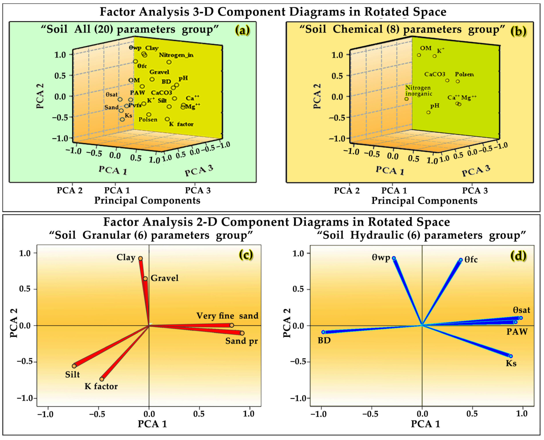
3.5. Factor Analysis Results and Discussion of Soil’s Chemical, Granular and Hydraulic Groups

Factor analysis endeavors to discover a way to detect the hidden parameters that may explain the correlational structure of a set of initial (observable) parameters. This modeling approach is commonly employed to compact the existing information within the initial parameters and further decrease the set of parameters in a dataset with minimal information losses; however, it may equally be deployed to investigate the latent structure of parameters in a raw data stream [9,83]. In our study, first multivariate factor analysis and then multivariate R-mode (rotated) factor analysis were performed to extract the factors governing the soil’s chemical, granular, and hydraulic parameters in the experimental field.

The R-mode multivariate factor analysis [9,76,78,83] was performed using as an extraction method the principal components analysis (PCA) [76,78,83] and as a rotation method the varimax method with Kaiser normalization [3,9,83,84,85] by utilizing the measured and analyzed lab data (soil’s chemical, granular, and hydraulic parameters) on GIS parametric maps in order to extract the factors or components (management zones) of the experimental field. The data matrix of 20 parameters and 144 data observations for each parameter was utilized in this factor analysis. The results of the statistical PCA analysis for the “soil All Parameters group” are reported in

Table 5. Factors, description of the component, variance (%), cumulative variance (%) results of the Principal Component Analysis (n = 144 for each parameter).

SN	Factor (PCA)	Description of Component	Variance (%)	Cumulative Variance (%)
1	Factor 1	‘Mg-Ca-CaCO3-Sand-pH-K factor-Vfs-Clay’	28.798	28.798
2	Factor 2	‘θwp-silt-θfc-nitrogen inorganic-Polsen’	22.725	51.523
3	Factor 3	‘θsat-PAW-Ks-BD’	17.693	69.216
4	Factor 4	‘organic matter and potassium K’	9.976	79.192
5	Factor 5	‘gravel’	5.815	85.006

and depicted graphically in a three-dimensional (3-D) component diagram (Figure 4a) in rotated space, aiming to uncover and explain relationships numerically and graphically between the 20 interacting soil parameters and to show trends of soil data in rotated 3-D space. Similarly, the results of the statistical PCA analysis for the “soil Chemical parameters group” are depicted graphically in a three-dimensional (3-D) component diagram (Figure 4b) in rotated space.

The results of the statistical PCA analysis for the “soil Granular parameters group” and the “soil Hydraulic parameters group” are depicted graphically in two-dimensional (2-D) component diagrams in rotated space (Figure 4c,d), respectively. The 3-D component diagram in rotated space (Figure 4a) depicts the spatial distribution and loadings of the 20 examined parameters in rotated three-dimensional space, showing the trends and loadings of the data centroids of the primary three PCs (factors) that account for 69.216% of the overall variance in the data matrix.

The initial determination of the optimum total of components (factors) was found to be the number of five components, or in our case, management zones.

• Factor-1 contains significant loadings of 8 parameters, and it can be considered a ‘Mg-Ca-CaCO₃-Sand-pH-K factor-Vfs-Clay’ component that explains the synergistic soil chemistry interactions between the 8 parameters as the dominating chemical processes in the field’s soil. The presence of high levels of calcium Ca⁺⁺ (0.838) and magnesium Mg⁺⁺ (0.852) loadings and concentrations in the soil is associated with the intensive farming activities taking place in the area. The soil of the trial field was categorized as alkaline, with pH values between 7.45 and 8.13.
• Factor-2 as a ‘θwp-silt-θfc-nitrogen inorganic-Polsen’ component explains hydraulic and chemical interactions between the above-mentioned five parameters. This factor is mainly represented by positive high loadings of θwp (0.920), silt (0.872), θfc (0.855), and nitrogen inorganic (0.803), and a negative loading of phosphorus (−0.419). Inorganic nitrogen does not have a significant lithologic origin at the site and may be related to the agricultural activities of the region and the surface runoff of nitrogen fertilizers.
• Factor-3 is considered a ‘θsat-PAW-Ks-BD’ component that exhibits a negative loading of bulk density (−0.984) relative to the saturated hydraulic conductivity Ks (0.838), as would be expected, and high positive loadings of PAW (0.894) and θsat (0.985).
• Factor-4 may be considered an ‘organic matter and potassium K’ component that exhibits high loadings of OM (0.918) and potassium K⁺ (0.891).
• The factor-5 is less significant and accounts for only 5.815% of the overall variance in the data matrix. This factor is considered a ‘gravel’ component that exhibits a high loading of gravel content (0.784), indicating that this factor is rock weathering.

The primary four main factors accounted for 79.192% of the overall variance in the data matrix and dominated against the rest of the components in the control of soil chemistry in the trial field. The remaining one main factor accounts for 5.815% of the variance, and the overall five-factor loadings, summed together, explain 85.006% of the total variance in the data matrix. The field’s optimal number of management zones was obtained based on factor and PCA R-mode analyses of the various soil parameter groups, 3-D and 2-D component diagrams in rotated space (Figure 4a–d), and the realistic potential of MZs application in the trial pattern. The factor analysis results (Table 5) of the “soil All parameters” group data indicated that the suggested optimum total of components (factors) was initially five, or in our case, five management zones.

The factor analysis outcomes of individual “soil Chemical parameters group," “soil Granular parameters group,” and “soil Hydraulic parameters group” data indicated that the suggested optimum total of components (MZs) were found to be three, two, and two, respectively. Since factor-5 is less significant than the others and accounts for only 5.815% of the overall variance, and for reasons of the realistic potential of MZs application in the trial field, it was finally chosen to apply four management zones in the trial field.

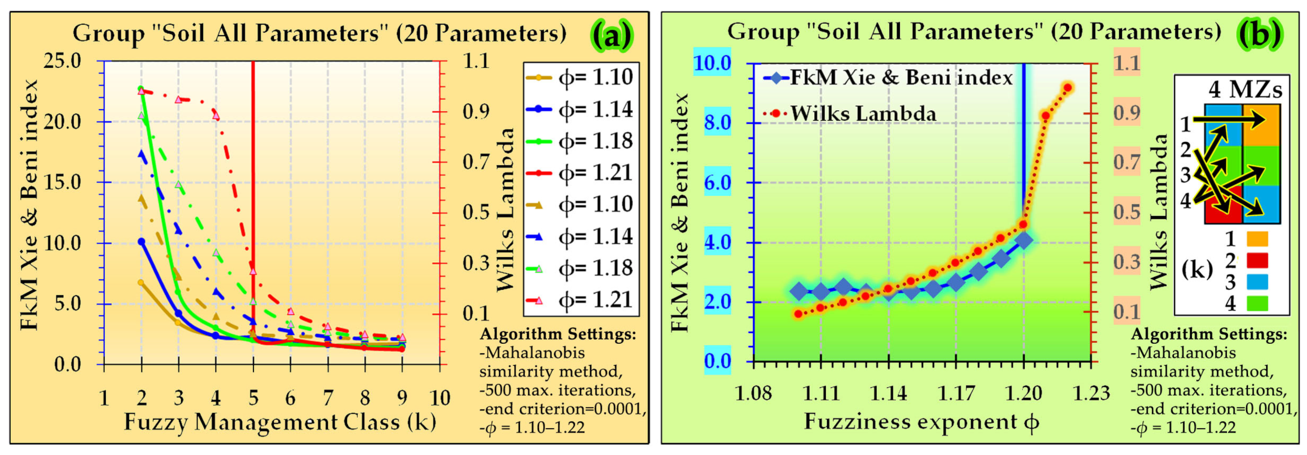
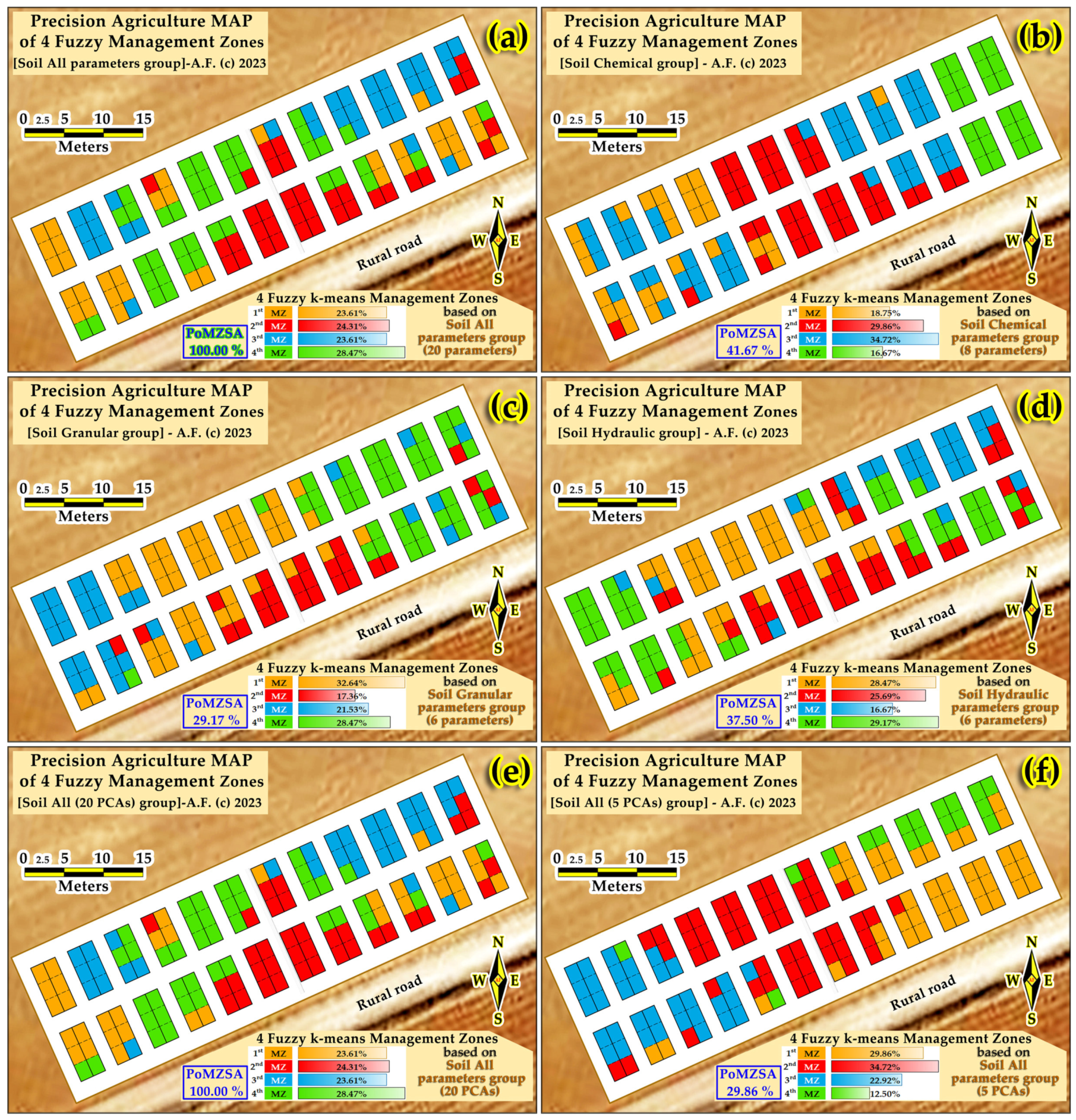
3.6. Delineating Field’s Management Zones Results and Discussion

The widespread diversity of soil nutritional, granular, and hydraulic parameters justifies the classification of these parameters into various categories so as to detect and delineate homogenous field zones (MZs) for their proper management. They were clustered into various categories based on their extent, represented by their magnitude, and the extent of each category was assessed. Fuzzy k-means clustering [51,52,53,54,55,56,57,58,59,60,61,62,63,64,65] was performed initially with the FuzME 3.5c software [62] and with the Management Zone Analyst (MZA) 1.01 software [63] in order to cluster the various soil parametric data into potential factors (MZs) and compare them. Finally, it was chosen to use the FuzME 3.5c software [62] because of its better options. First, an exploratory Fuzzy k-means clustering [51,52,53,54,55,56,57,58,59,60,61,62,63,64,65] analysis was conducted to clarify which distance metric and fuzziness exponent φ were better to use with the available field soil data. Multiple runs of the software were performed in order to evaluate the results of various cases and select the best distance metric and fuzziness exponents φ for further use in the analysis. Based on the nature and characteristics of the field data, the results of the software’s multiple runs, and the structure of each variance-covariance matrix, the Mahalanobis similarity distance metric was selected for multivariate clustering. Then, multiple runs of the Fuzzy algorithm [51,52,53,54,55,56,57,58,59,60,61,62,63,64,65] with varying fuzziness exponent φ from 1.10 to 2.00 were performed. Based on the multivariate clustering results, the calculated indices of fuzzy performance index (FPI), modified partition entropy (MPE) [51,55,62], Xie & Benny’s k-means fuzzy index (FkM Xie & Benny’s index) [59] and Wilks lambda [3,62,78] vs. the varying fuzziness exponent φ were utilized to identify the optimal φ and number of MZs. The various indexes that result from the fuzziness exponent’s φ evaluation are depicted in Figure 5a,b.

The results of the exploratory Fuzzy k-means clustering [51,52,53,54,55,56,57,58,59,60,61,62,63,64,65] analysis and the various indexes reveal that the tested fuzziness exponent φ from 1.10 to 2.00 of the group data “soil All parameters” was found valid only in the range between 1.10 and 1.21 (see Figure 5a,b). Over this valid range of φ values, the optimal fuzziness exponent found was φ = 1.14, and the optimal number of management zones found was k = 4.

Similar results on the fuzziness exponent φ have been reported by other studies [58,59,60].The Fuzzy k-means algorithm [51,52,53,54,55,56,57,58,59,60,61,62,63,64,65] was run with parameter settings as follows: Metric distance: Mahalanobis similarity method for multivariate clustering, fuzziness exponent φ = 1.14, maximum iterations = 500, stopping criterion = 0.0001, and random start with membership variance = 0.1. Based on the Fuzzy algorithm results, the “soil All parameters group” map with 4 MZs (Figure 6a) for the experimental field was produced, and the extent (in %) of each MZ was assessed, along with the fuzzy clustering metric Percentage of Management Zones Spatial Agreement (PoMZSA) (%) between soil groups.

Similarly, another Fuzzy k-means grouping in 4 MZs was carried out with soil’s chemical and nutritional parameter data (“soil chemical group” consisted of 8 parameters) using a fuzziness exponent φ = 1.14 (found to be the optimal φ for 4 MZs and the group’s structure), and the output 4 MZs map and the extent (in %) of each MZ are depicted in Figure 6b. Based on the soil’s “granular group” (6 parameters), the Fuzzy algorithm grouping in 4 MZs was carried out with a fuzziness exponent φ = 1.26 (found optimal φ for 4 MZs and the group’s structure), yielding an output map with 4 MZs (Figure 6c). Finally, based on the soil’s “hydraulic group” (6 parameters), the Fuzzy algorithm grouping in 4 MZs was carried out with a fuzziness exponent φ = 1.48 (optimal φ for 4 MZs and the group’s structure), resulting in the output map with 4 MZs in Figure 6d.

Regarding evaluation indexes, the combination of the lower values of FPI and MPE [51,55,62], is considered the best. Moreover, the lower values of Xie & Benny’s k-means fuzzy index (FkM Xie & Benny’s index) [59] and Wilks’ lambda [3,62,78] are considered the best. By analyzing the data, the MZ output maps of the field, and the various evaluation indexes, we concluded that the four MZ output maps in the “soil All parameters group” (Figure 6a) were supplying the higher clustering insight of the field’s soil data and nutrients. Based on the exploratory fuzzy analysis results when FPI and MPE values were confusing for a final decision, the FkM Xie & Benny’s index (lowest value) was proven to be robust and pointed clearly to the optimal fuzziness exponent for the recommended MZs.

The 4 MZs field map based on the “soil All parameters group” (20 parameters) in Figure 6a was regarded as the “reference map” for all maps. Moreover, a comparison between the various soil parameters and fuzzy clustering results was performed. The fuzzy algorithm comparison was conducted on 4 MZs maps outcomes between 6 groups of various soil parameters (

Table 6. Fuzzy clustering Percentage of Management Zones Spatial Agreement.

SN	Soil Parameters Group	Optimal Fuzziness Exponent φ	Fuzzy Clustering Percentage of Management Zones Spatial Agreement (PoMZSA) (%) between Soil Groups
			MZ 1	MZ 2	MZ 3	MZ 4	All MZs
1	“soil All parameters group” (20 parameters), 4 MZs	1.14	100.00	100.00	100.00	100.00	100.00
2	“soil All parameters group” (20 PCAs), 4 MZs	1.14	100.00	100.00	100.00	100.00	100.00
3	“soil All parameters group” (5 PCAs), 4 MZs	1.56	40.00	60.00	20.59	2.44	29.86
4	“soil chemical group” (8 parameters), 4 MZs	1.14	35.29	74.29	61.76	2.44	41.67
5	“soil granular group” (6 parameters), 4 MZs	1.26	11.76	57.14	35.29	14.63	29.17
6	“soil hydraulic group” (6 parameters), 4 MZs	1.48	11.76	77.14	55.88	9.76	37.50

), using the fuzzy clustering metric: Percentage of Management Zones Spatial Agreement (PoMZSA) (%) between soil group maps and MZs.

The results of the analysis showed that PoMZSA (%) between soil groups varied greatly. Only the 4 MZs map of the “soil All parameters group” with 20 PCAs (output from the principal components analysis) map (Figure 6e) resulted in 100.00% spatial agreement of the 4 MZs with the “reference map” (Figure 6a). On the contrary, the 4 MZs map of the “soil All parameters group” with 5 PCAs (output from the PCA analysis with 5 factors) (Figure 6f), although that explained 85.006% of the total variance in the group data matrix, resulted in a low PoMZSA = 29.86% of management zone spatial agreement with the “reference map” (Figure 6a).

The outcome of fuzzy k-means clustering algorithm comparison of the developed 4 MZs maps of “soil chemical group” (8 parameters) in Figure 6b, “soil granular group” (6 parameters) in Figure 6c, and “soil hydraulic group” using 6 parameters (Figure 6d) resulted in 3 different low PoMZSAs, i.e., 41.67%, 29.17%, and 37.50%, respectively. Hereby, it is worth noting that the 2nd MZ of each of the 3 soil groups presented the highest spatial agreement with the 2nd MZ of the “reference map," with PoMZSAs of 74.29%, 57.14%, and 77.14%, respectively. On the contrary, the 4th MZ of each of the 3 group maps presented a low spatial agreement with the 4th MZ of the “reference map," with low PoMZSAs of 2.44%, 14.63%, and 9.76%, respectively.

Based on the fuzzy k-means clustering algorithm comparison results between groups, it was concluded that only the 4 MZs map of the “soil All parameters group” map (Figure 6e), with 20 PCAs (output from the principal components analysis that explain 100.00% of the total variance in the group data matrix), resulted in 100.00% spatial agreement of management zones with the “reference map” (Figure 6a). All the other soil parameter groups presented low to medium PoMZSAs. Thus, in the k-means fuzzy clustering methodology, based on the results of our study, it is concluded that it is better to use the full parameter dataset or the full PCAs dataset of variables in order to obtain insightful and better field management zone maps with high PoMZSAs.

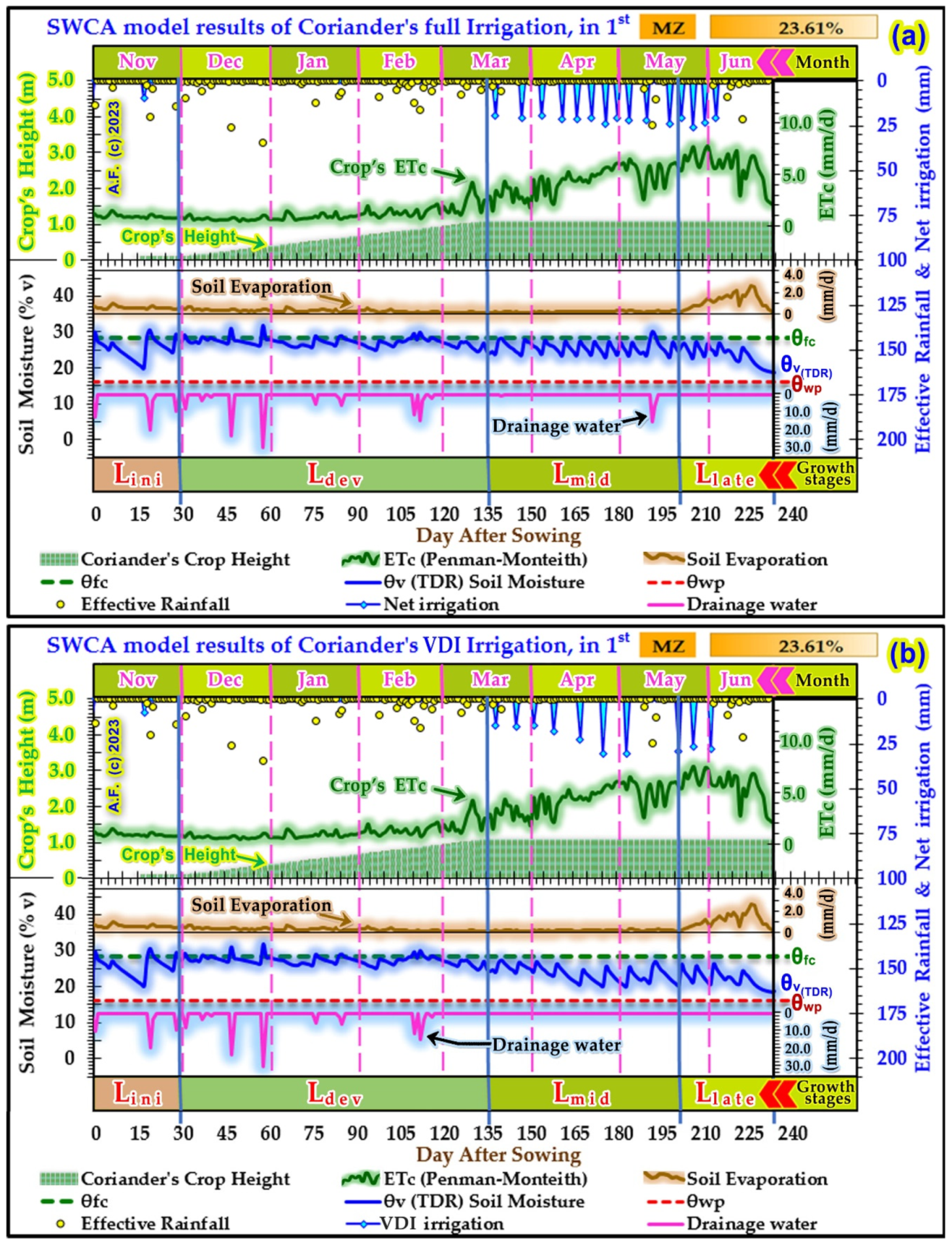
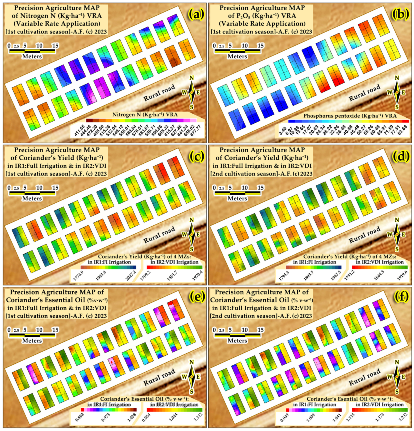
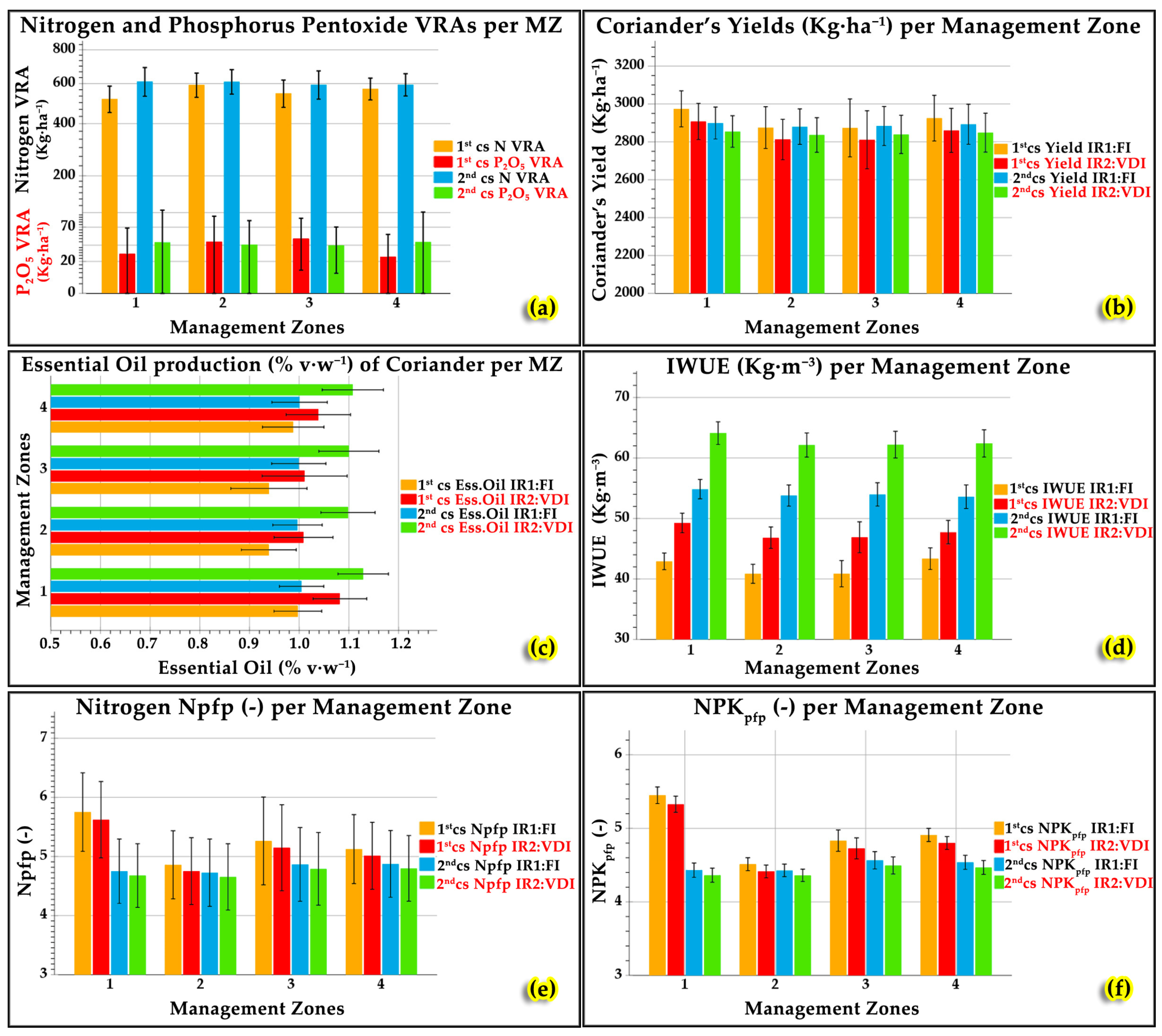
3.7. Results and Discussion of Soil–Water–Crop–Atmosphere (SWCA) and ASMD Model, the Deficit Irrigation and VRA Effects on Field’s Management Zones Yields and Essential Oil

VDI is described as an irrigation control operation strategy in which plants are watered with a reduced amount that is usually lower than the total crop demands (actual evapotranspiration) for optimum crop growth in an effort to decrease the overall irrigation water volume applied, enhance the plants’ responsiveness to water deficit in a beneficial way, and thereby raise the crop’s IWUE. In the current research, we classify the water deficit according to soil water level into six classes as they are defined in [18]: (1) Severe water deficit (<50% of ${\theta }_{fc}$), (2) Moderate water deficit (50–60% of ${\theta }_{fc}$), (3) Mild water deficit (60.1–75% of ${\theta }_{fc}$), (4) Light water deficit (75.1–90% of ${\theta }_{fc}$), (5) No deficit or full irrigation (>90% of ${\theta }_{fc}$), and (6) Over-irrigation (>100% of ${\theta }_{fc}$). The length in days of the initial or seedling growth stage (Lini) [14] lasted 30 days, extending from the seeding day (early November) until almost 10% topsoil coverage of coriander. Over the Lini stage, the θpini of the SWCA-model was fixed at 0.65, i.e., MAD (Management Allowable Depletion) = 65% [14,17,18,25]), for coriander growing without water stress. MAD defines the amount of SM that can be consumed prior to being renewed by irrigational water. The lifespan of the flowering stage (Ldev) [14,17,25] was 105 days, with a trend from 10% topsoil cover of leafy greening to complete topsoil covering. The actual full coverage of the crop typically happens at the onset of flowering. The mid-season stage (Lmid) length [14,17] was 68 days, extending from the actual topsoil total coverage to the onset of plant maturation. The late season or maturation stage (Llate) [14,17] was 30 days, extending from the onset of plant maturity to harvesting of the crop or complete senescence (Figure 7a,b). Soil moisture is the foremost contributor to enhancing the development and productivity of crops under rainfed and irrigated regimes. Considering the various growth stages, the reproductive stadia (Lmid and Llate) are far more fragile than the vegetative.

For the 1st cultivation season, the representative Figure 7a,b depict the results of the day-to-day SWCA and ASMD models [3,14,17,18,25] by observing the day-to-day SM monitor of ${\theta }_{V\left(TDR\right)}$ (obtained from a TDR instrument with multisensors [18,20,21,25,72,73]), the precipitation, the variable deficit irrigation, the height progression and evapotranspiration of coriander, the field capacity ${(\theta }_{fc})$, the saturation ${\theta }_S$, the permanent wilting point (${\theta }_{wp})$, topsoil evaporation, and deep percolation (drainage water) throughout the 4 crop growth stages of the first management zone for IR1:Full and IR2:VDI irrigation levels, respectively), November’s prevailing climatic conditions during the coriander’s seedling growth stage [14,17,25] were favorable in the 1st cultivation season, and limited water quantity was needed to be supplied to IR1-MZ1:Full (21.07 mm) and in IR2-MZ1:VDI (15.80 mm) and accordingly to the rest of the 3 MZs. In the IR1:Full and IR2:VDI irrigation of all MZs, throughout the coriander’s Lini growing stage, a moderate to mild VDI (60–75%) was applied, and plant observations were utilized. The prevailing climatic conditions of the 1st cultivation period (where frequent rainfall occurred) throughout the flowering stage (Ldev) [14,17,25] (December to the middle of March) in the field area were favorably suited since no irrigation was required in any management zone. This favorable situation is due to Pef = 58.66 mm of Lini and Pef = 194.45 mm of Ldev lifespans. In fact, for the Ldev stage, the effective rainfall turned out to be adequate to match the ETc and ETα, which were determined using the SWCA model to be 99.00 mm for both the IR1-MZ1:Full and IR2-MZ1:VDI and the other MZ treatments. In the IR1:Full and IR2:VDI irrigation levels of all MZs, throughout the coriander’s Lmid growing stage, a moderate to mild VDI (60–75%) was supplied, and plant observations were utilized (Figure 7a,b). The detailed SWCA and ASMD model outcomes of the 1st growing season for the 4 management zones are reported in

Table 7. First cultivation season outcomes of SWCA and depletion (ASMD) models for the 4 management zones of the experimental field.

Management Zones Results of the SWCA and the Depletion Models of Coriandrum sativum L. in 1st c.s.
Parameter	1st MZ		2nd MZ		3rd MZ		4th MZ
Season duration in days	233		233		233		233
Irrigation treatment	IR1:Full	IR2:VDI	IR1:Full	IR2:VDI	IR1:Full	IR2:VDI	IR1:Full	IR2:VDI
Water deficit [%]	100%	60–75%	100%	60–75%	100%	60–75%	100%	60–75%
ASMD average [%]	17.89	24.69	18.13	24.25	18.36	24.48	18.87	24.16
ASMD max [%]	75.77	80.24	83.71	83.72	84.80	84.80	80.76	80.76
Ks average [–] *	0.976	0.913	0.976	0.920	0.975	0.918	0.968	0.919
Ks max [–]	1.000	1.000	1.000	1.000	1.000	1.000	1.000	1.000
Ks min [–] *	0.355	0.269	0.366	0.240	0.361	0.236	0.287	0.259
Ks-weighted average [–] *	0.936	0.842	0.936	0.852	0.935	0.850	0.924	0.852
Number of days with Ks < 1 *	38	73	38	69	38	69	42	68
Percentage of days with Ks < 1 *	16.31	31.33	16.31	29.61	16.31	29.61	18.03	29.18
Net Irrigation NIR [mm]	348.74	246.05	359.38	256.30	358.82	255.10	330.35	254.85
Effective rainfall Pe = P-RO [mm]	344.28	344.28	344.28	344.28	344.28	344.28	344.28	344.28
TWI = (NIR + Pe) [mm]	693.02	590.34	703.66	600.59	703.10	599.39	674.63	599.14
ETc [mm/stage]	564.44	559.85	564.25	559.01	564.12	558.89	562.07	558.77
ETα [mm/stage]	546.28	474.46	546.24	479.03	545.27	477.19	537.36	478.74
Deep percolation DP [mm]	177.70	149.76	183.71	151.64	183.74	151.81	167.50	151.50
DP (% losses of NIR)	50.96	60.87	51.12	59.16	51.21	59.51	50.70	59.45
DP (% losses of TWI)	25.64	25.37	26.11	25.25	26.13	25.33	24.83	25.29
TWI-DP [mm]	515.32	440.58	519.95	448.95	519.36	447.58	507.13	447.64
Kcb average	0.83	0.83	0.83	0.83	0.83	0.83	0.83	0.83
Kcb deviation	0.30–1.19	0.30–1.19	0.30–1.19	0.30–1.19	0.30–1.19	0.30–1.19	0.30–1.19	0.30–1.19
Kc average	1.15	1.14	1.15	1.14	1.15	1.14	1.14	1.14

(*) Ks < 1 indicates water stress to plants.

.

In the IR1:Full and IR2:VDI irrigation levels of all MZs, throughout the coriander’s late or maturation stage [14,18], a mild DI (75%) was supplied, and plant observations were utilized. In the entire 1st growth season, the daily SWCA and depletion model results of each one of the 4 MZs and the SM results pointed to the overall water quantities supplied to the 4 MZs in IR1: Full irrigation that ranged from 674.63 to 703.66 mm. The ETc ranged from 562.07 to 564.44 mm, the ETα ranged from 537.36 to 546.28 mm, and drainage ranged from 167.50 to 183.74 mm, demonstrating 24.83 to 26.13% losses to the supplied overall water (full irrigation + effective precipitation). The SWCA model’s results for the 4 MZs showed that, in IR1:FI, the Ks-average coefficient ranged from 0.913 to 0.920 and in IR2:VDI from 0.968 to 0.976, respectively. If Ks-average present values are lower than unity, this indicates that water stress is occurring on plants [3,17,18,25]. Regarding the various water inputs applied to the 4 MZs in IR2:VDI irrigation (590.34 to 600.59 mm), the ETc, the actual evapotranspiration, and drainage outcomes demonstrated 25.25 to 25.37% losses of overall supplied quantity (VDI + effective precipitation) due to frequently high precipitations in Lini and Ldev srages.

The detailed outcomes of the SWCA and ASMD models of the 2nd cultivation season for the 4 management zones are reported in

Table 8. Second cultivation season outcomes of SWCA and depletion (ASMD) models for the 4 management zones of the experimental field.

Management Zones Results of the SWCA and the Depletion Model of Coriandrum sativum L. in 2nd c.s.
Parameter	1st MZ		2nd MZ		3rd MZ		4th MZ
Season duration in days	233		233		233		233
Irrigation treatment	IR1:Full	IR2:VDI	IR1:Full	IR2:VDI	IR1:Full	IR2:VDI	IR1:Full	IR2:VDI
Water deficit [%] of ${\theta }_{fc}$	100%	60–75%	100%	60–75%	100%	60–75%	100%	60–75%
ASMD average [%]	20.99	28.17	19.57	27.30	19.51	27.42	19.29	27.11
ASMD max [%]	81.96	87.28	84.53	85.11	85.61	85.62	83.34	84.30
Ks average [–] *	0.960	0.904	0.954	0.906	0.953	0.906	0.957	0.908
Ks max [–]	1.000	1.000	1.000	1.000	1.000	1.000	1.000	1.000
Ks min [–] *	0.233	0.135	0.183	0.167	0.178	0.164	0.203	0.185
Ks-weighted average [–] *	0.918	0.825	0.910	0.831	0.909	0.830	0.913	0.834
Number of days with Ks < 1 *	41	81	43	78	43	78	43	76
Percentage of days with Ks < 1 *	17.60	34.76	18.45	33.48	18.45	33.48	18.45	32.62
Net Irrigation NIR [mm]	308.54	225.25	315.39	236.43	314.19	236.43	319.75	236.39
Effective rainfall Pe = P−RO [mm]	220.03	220.03	220.03	220.03	220.03	220.03	220.03	220.03
TWI = (NIR + Pe) [mm]	528.57	445.29	535.42	456.46	534.22	456.46	539.79	456.42
ETc [mm/stage]	521.97	520.57	521.46	519.50	521.38	519.43	521.42	519.46
ETα [mm/stage]	493.03	435.44	488.70	436.58	487.82	436.01	491.01	436.86
Deep percolation DP [mm]	70.36	47.57	78.05	51.61	77.24	51.64	81.23	52.49
DP (% losses of NIR)	22.80	21.12	24.75	21.83	24.58	21.84	25.40	22.21
DP (% losses of TWI)	13.31	10.68	14.58	11.31	14.46	11.31	15.05	11.50
TWI-DP [mm]	458.21	397.71	457.37	404.85	456.98	404.82	458.56	403.93
Kcb average	0.83	0.83	0.83	0.83	0.83	0.83	0.83	0.83
Kcb deviation	0.30–1.18	0.30–1.18	0.30–1.18	0.30–1.18	0.30–1.18	0.30–1.18	0.30–1.18	0.30–1.18
Kc average	1.13	1.13	1.13	1.12	1.13	1.12	1.13	1.12

(*) Ks < 1 indicates water stress to plants.

.

In the entire 2nd growth season, the daily SWCA and ASMD model results of each one of the 4 management zones and the SM results revealed that overall water quantities supplied to the 4 MZs in IR2:VDI irrigation ranged from 445.29 to 456.46 mm, that is 75.43% to 76.00% of the first’s season total water inputs (590.34 to 600.59 mm), and the ETc ranged from 519.43 to 520.57 mm, that is 92.95% to 92.98% of the first’s season ETc (558.77 to 559.85 mm). In IR2:VDI irrigation, the actual evapotranspiration comparison of the two cultivation seasons showed that the ETα of the second c.s. was 91.78% to 91.20% of the first’s season ETα, and the deep percolation was 31.76% to 34.02% of the first’s season deep percolation, demonstrating 10.68 to 11.50% losses to the supplied overall water quantities (NIR irrigation + effective precipitation). Management zones and VDI irrigation, if implemented prudently at critical development stages, could lead to significant water savings improvements. The water savings results of VDI irrigation in comparison with full irrigation application between the 2 growth seasons ranged from 22.85% up to 29.44% in the 1st cultivation season and from 25.03% up to 26.99% in the 2nd cultivation season of coriander. The results of water savings from VDI irrigation in comparison with full irrigation in the various management zones for the 2 growing seasons were statistically significant for all MZs and ranged for the 1st MZ from 26.99% up to 29.44%, for the 2nd MZ from 25.03% up to 28.68%, for the 3rd MZ from 25.73% up to 28.90%, and for the 4th MZ from 22.85% up to 26.07%.

The average amounts of soil properties for each management zone and the VRA mean for the 1st and 2nd c.s. of the experimental field are presented in

Table 9. Mean values of soil parameters and nitrogen and phosphorus pentoxide VRA applications per management zone of the experimental field.

SN	Parameter	1st MZ	2nd MZ	3rd MZ	4th MZ
1	Calcium Ca++ (mg·kg−1)	2233.121	1896.783	2391.906	2399.249
2	Calcium carbonate CaCO3 (%)	1.862	0.968	1.700	1.742
3	Magnesium Mg++ (mg·kg−1)	1969.192	1660.571	1964.776	1995.331
4	Nitrogen inorganic(mg·kg−1)	76.151	59.622	75.192	62.752
5	Organic matter (%)	1.789	1.676	1.939	1.763
6	pH [1:2 soil/water solution]	7.878	7.744	7.851	7.813
7	Phosphorus P-olsen (mg·kg−1)	16.643	15.274	14.559	17.123
8	Potassium K+ (mg·kg−1)	405.655	403.556	409.28	417.689
9	Clay (size: <0.002 mm) (%)	25.349	25.052	25.317	23.814
10	Gravel (%)	0.083	0.093	0.077	0.057
11	Sand pr (size: 0.2–2 mm) (%)	32.367	34.386	32.728	33.873
12	Silt (size: 0.002–0.02 mm) (%)	20.357	18.545	19.441	20.229
13	Soil Erodibility (Mg·ha·h·ha−1·MJ−1·mm−1)	0.0309	0.0301	0.0301	0.0313
14	Vfs sand (size: 0.02–0.2 mm) (%)	21.868	22.010	21.903	21.981
15	Bulk density (g·cm−1)	1.386	1.411	1.469	1.397
16	Field capacity θfc (m3·m−3)	28.536	27.528	27.640	27.072
17	Plant available water PAW (cm·cm−1)	0.1146	0.1081	0.1066	0.1138
18	Sat. Hydraulic conductivity Ks (mm·h−1)	16.634	16.368	11.719	19.676
19	Saturation θsat (m3·m−3)	47.991	46.762	44.454	47.362
20	Wilting point θwp (m3·m−3)	16.257	15.989	16.364	15.426
21	Nitrogen (kg·ha−1) VRA mean (1st c.s.)	518.985	593.528	548.310	572.270
22	Nitrogen (kg·ha−1) VRA mean (2nd c.s.)	612.402	611.334	594.916	595.160
23	P2O5 (kg·ha−1) VRA mean (1st c.s.)	28.648	45.290	49.929	25.168
24	P2O5 (kg·ha−1) VRA mean (2nd c.s.)	44.404	40.761	39.943	44.799

.

The variable rate application (VRA) allows the spreading of a predetermined dose of fertilizer to each management zone, depending on the results of the soil analyses. The applied fertilizer VRA is a promising method in PA that can reduce nitrogen and other nutrient amounts, such as phosphorus pentoxide and potassium oxide, decrease economic costs, and reduce nitrogen leaching. Thus, we chose VRA fertilization under full (IR1:FI) and variable deficit irrigation (IR2:VDI) for nitrogen and P₂O₅ in each MZ (Figure 8a,b) and statistically investigated the coriander yields of the different management zone results (4 MZs). As for the potassium oxide fertilization, it was decided not to apply it due to the presence of elevated potassium K⁺ levels found in the laboratory analyses (see Table 1) and reflected in field soil mapping results (Figure 3f).

Additionally, nitrogen and phosphorus pentoxide VRA (variable rate applications) mean per management zone of the experimental field for the 1st and 2nd cultivation seasons (c.s.) are presented in Table 9. In many of the soil parameters, significant differences are observed between the four management zones of the experimental field.

Examples of nitrogen and P₂O₅ variable rate application (VRA) prescription maps of the first cultivation season are depicted in Figure 8a [nitrogen (kg·ha⁻¹) VRA prescription map] and in Figure 8b [phosphorus pentoxide (kg·ha⁻¹) VRA prescription map]. Taking into consideration the two cultivation seasons of the coriander, it is noticed that in the 1st c.s., the nitrogen and phosphorus pentoxide variable rate application prescription maps present a higher standard deviation and a higher range than those of the 2nd season.

Moreover, Figure 8c,d depicts the harvesting results of the fruit yield PA maps of IR1: Full irrigation and IR2: VDI irrigation in the 1st cultivation season and the fruit yield PA maps of IR1: FI and IR2: VDI irrigation in the 2nd cultivation season, respectively. Additionally, in Figure 8e,f are depicted the essential oil production (% v·w⁻¹) PA map of IR1:FI and IR2:VDI irrigation in the 1st c.s. and the essential oil production (% v·w⁻¹) PA map of IR1:FI and IR2:VDI irrigation in the 2nd c.s., respectively.

The unbalanced one-way ANOVA (p = 0.05) [3,9,67,76,78] revealed that the 4 management zones—which have different soil nutrients and other soil parameters—as de facto treatments obtained by PA with a fuzzy k-means clustering algorithm, with the 2 irrigation levels [MZx-IR1: full irrigation, MZx-IR2: variable deficit irrigation], in the 1st cultivation season significantly affected the coriander’s yield (kg·ha⁻¹) and the essential oil production (% v·w⁻¹). On the contrary, in the 2nd cultivation season, the 4 MZs as de facto treatments did not result in significant differences in coriander’s yield (kg·ha⁻¹). The statistical analysis for the 4 MZs effects and irrigation levels results for the coriander yield and essential oil production of the 1st and 2nd c.s. are presented in

Table 10. Statistical analysis (ANOVA (p = 0.05)) for MZs effects and irrigation level results for the coriander yield and essential oil production.

Dependent Variable	C.s.	MZs	Irrigation Level	Management Zones Effects	Sum of Squares	df	Mean Square	F	Sig.
coriander_YIELD1_FI	1st		IR1:FI	Between Groups	235,792.892	3	78,597.631	21.296	0.000
		4		Within Groups	516,711.442	140	3690.796
				Total	752,504.333	143
coriander_YIELD1_VDI	1st		IR2:VDI	Between Groups	219,431.814	3	73,143.938	20.471	0.000
		4		Within Groups	500,228.460	140	3573.060
				Total	719,660.275	143
coriander_YIELD2_FI	2nd		IR1:FI	Between Groups	7959.955	3	2653.318	1.118	0.344
		4		Within Groups	332,194.483	140	2372.818
				Total	340,154.438	143
coriander_YIELD2_VDI	2nd		IR2:VDI	Between Groups	7285.969	3	2428.656	1.069	0.364
		4		Within Groups	318,066.413	140	2271.903
				Total	325,352.381	143
Essential_Oil_1_FI	1st		IR1:FI	Between Groups	0.103	3	0.034	36.645	0.000
		4		Within Groups	0.132	140	0.001
				Total	0.235	143
Essential_Oil_1_VDI	1st		IR2:VDI	Between Groups	0.119	3	0.040	35.515	0.000
		4		Within Groups	0.156	140	0.001
				Total	0.275	143
Essential_Oil_2_FI	2nd		IR1:FI	Between Groups	0.001	3	0.000	0.618	0.604
		4		Within Groups	0.093	140	0.001
				Total	0.094	143
Essential_Oil_2_VDI	2nd		IR2:VDI	Between Groups	0.020	3	0.007	8.215	0.000
		4		Within Groups	0.115	140	0.001
				Total	0.135	143

.

The results of the 4 MZs treatments for various observed parameters for the 1st and 2nd seasons are presented in the 6 diagrams of Figure 9. Moreover, the unbalanced one-way ANOVA (p = 0.05) [3,9,67,76,78] outcomes revealed coriander’s yields of 1st c.s. [means: MZ1–MZ4 for IR1:FI = 2912.79 (±72.54) kg·ha⁻¹, MZ1–MZ4 for IR2:VDI = 2848.61 (±70.94) kg·ha⁻¹], were affected significantly by management zone and by irrigation level. The coriander’s yields of 2nd c.s. [means: MZ1–MZ4 for IR1:FI = 2889.50 (±48.77) kg·ha⁻¹, MZ1–MZ4 for IR2:VDI = 2845.15 (±47.70) kg·ha⁻¹], were not affected significantly by either management zone or irrigation level.

It took two cultivation seasons for the different nitrogen and phosphorous pentoxide fertilizer VRAs (Variable Rate Application) that were applied in the field to leverage the nutrients in the soil levels and present homogenous coriander yields (kg·ha⁻¹) between the 4 MZs with statistically non-significant differences in the 2nd c.s. (Table 10).

Additionally, the unbalanced one-way ANOVA (p = 0.05) [3,9,67,76,78] results showed that the essential oil production of the 1st c.s. [means: MZ1–MZ4 for IR1:FI = 0.967 (±0.041)% v·w⁻¹, MZ1–MZ4 for IR2:VDI = 1.035 (±0.044)% v·w⁻¹], was significantly affected by management zone and by irrigation level. The coriander’s essential oil production in 2nd c.s. [means: MZ1–MZ4 for IR1:FI = 1.0004 (±0.026)% v·w⁻¹, MZ1–MZ4 for IR2:VDI = 1.1088 (±0.031)% v·w⁻¹], were not affected significantly by either management zone or irrigation in full irrigation level (IR1:FI); however, were affected significantly by MZ and irrigation in VDI level (IR2:VDI). It is worth noting that, in both cultivation seasons, the essential oil production of the management zones was higher at the IR2:VDI level.

It was found that VDI leads to lower fruit yields but without significant differences (p = 0.05) among MZs when appropriate VRA fertilization is applied to leverage soil nutrient levels through different MZs, and also that VDI compared to full irrigation application in different management zones yields 22.85% up to 28.90% in irrigation water savings.

Regarding essential oil production, it is concluded that deficit irrigation (IR2:VDI) leads to higher essential oil production, with significant differences among full and VDI irrigation and management zones.

4. Conclusions

An agronomist can be greatly assisted in recognizing and locating field sites of low, medium, and high soil fertility by analyzing the PAs spatial variability maps of soil’s “Chemical Parameter Group” and comprehending the effect of each parameter on plants’ development. Moreover, in the k-means fuzzy clustering of the field’s management zone delineation methodology, it is concluded that it is better to use the full parameter dataset or the full PCAs dataset of variables in order to obtain more accurate MZs and insightful and better management zone maps with high PoMZSAs for high spatial agreement.

The unbalanced one-way ANOVA (p = 0.05) statistical analysis results revealed that correct delineation of management zones using precision agriculture with fuzzy k-means clustering, if applied under variable deficit irrigation and VRA fertilization, leads to increased essential oil content of coriander with statistically significant differences (SSD), and to lower fruit yields; however, without SSD differences among management zones, when appropriate VRA fertilization is applied to leverage soil nutrient levels through the different fuzzy clustered MZs, for farming sustainability. Moreover, VDI compared to full irrigation in different management zones yields 22.85% to 29.44% in water savings, thus raising IWUE (46.833 to 64.112 kg·m⁻³), nitrogen use efficiency (4.655 to 5.623), and N-P-K fertilizer productivity (4.361 to 5.329). Finally, a further course of action in research would be the trial of more VDI levels and more VRA levels under all MZs.

References

1. Küppers, M.; O’Rourke, L.; Bockelée-Morvan, D.; Zakharov, V.; Lee, S.; Von Allmen, P.; Carry, B.; Teyssier, D.; Marston, A.; Müller, T.; et al. Localized sources of water vapour on the dwarf planet (1). Ceres Nat. 2014, 505, 525–527. [Google Scholar] [CrossRef]
2. Siddique, K.H.M.; Bramley, H. Water Deficits: Development; CRC Press: Boca Raton, FL, USA, 2014; pp. 1–4. [Google Scholar] [CrossRef]
3. Filintas, A. Land Use Evaluation and Environmental Management of Biowastes, for Irrigation with Processed Wastewaters and Application of Bio-Sludge with Agricultural Machinery, for Improvement-Fertilization of Soils and Crops, with the Use of GIS-Remote Sensing, Precision Agriculture and Multicriteria Analysis. Ph.D. Thesis, University of the Aegean, Mitilini, Greece, 2011. [Google Scholar]
4. Gleick, P.H.; Palaniappan, M. Peak water limits to freshwater withdrawal and use. Proc. Natl. Acad. Sci. USA 2010, 107, 11155–11162. [Google Scholar] [CrossRef]
5. Shiklomanov, I.A. Appraisal and assessment of world water resources. Water Int. 2000, 25, 11–32. [Google Scholar] [CrossRef]
6. Schiermeier, Q. The parched planet: Water on tap. Nature 2014, 510, 326–328. [Google Scholar] [CrossRef]
7. Gan, Y.; Siddique, K.H.M.; Turner, N.C.; Li, X.-G.; Niu, J.-Y.; Yang, C.; Liu, L.; Chai, Q. Ridge-furrow mulching systems—An innovative technique for boosting crop productivity in semiarid rain-fed environments. Adv. Agron 2013, 118, 429–476. [Google Scholar] [CrossRef]
8. FAO. Coping with Water Scarcity: An Action Framework for Agriculture and Food Security; FAO: Rome, Italy, 2012; p. 100. [Google Scholar]
9. Stamatis, G.; Parpodis, K.; Filintas, A.; Zagana, E. Groundwater quality, nitrate pollution and irrigation environmental management in the Neogene sediments of an agricultural region in central Thessaly (Greece). Environ. Earth Sci. 2011, 64, 1081–1105. [Google Scholar] [CrossRef]
10. EEA. Use of Freshwater Resources in Europe, CSI 018; European Environment Agency (EEA): Copenhagen, Denmark, 2019. [Google Scholar]
11. Koutseris, Ε.; Filintas, A.; Dioudis, P. Antiflooding prevention, protection, strategic environmental planning of aquatic resources and water purification: The case of Thessalian basin, in Greece. Desalination 2010, 250, 318–322. [Google Scholar] [CrossRef]
12. Islam, S.M.F.; Karim, Z. World’s Demand for Food and Water: The Consequences of Climate Change. In Desalination-Challenges and Opportunities; Farahani, M.H.D.A., Vatanpour, V., Taheri, A.H., Eds.; IntechOpen: London, UK, 2019; Chapter 4; pp. 1–27. [Google Scholar] [CrossRef]
13. Filintas, A.; Wogiatzi, E.; Gougoulias, N. Rainfed cultivation with supplemental irrigation modelling on seed yield and oil of Coriandrum sativum L. using Precision Agriculture and GIS moisture mapping. Water Supply 2021, 21, 2569–2582. [Google Scholar] [CrossRef]
14. Siebert, S.; Kummu, M.; Porkka, M.; Döll, P.; Ramankutty, N.; Scanlon, B.R. A global data set of the extent of irrigated land from 1900 to 2005. Hydrol. Earth Syst. Sci. 2015, 19, 1521–1545. [Google Scholar] [CrossRef]
15. Garrote, L.; Iglesias, A.; Granados, A.; Mediero, L.; Martin-Carrasco, F. Quantitative assessment of climate change vulnerability of irrigation demands in Mediterranean Europe. Water Resour. Manag. 2015, 29, 325–338. [Google Scholar] [CrossRef]
16. Kreins, P.; Henseler, M.; Anter, J.; Herrmann, F.; Wendland, F. Quantification of climate change impact on regional agricultural irrigation and groundwater demand. Water Resour. Manag. 2015, 29, 3585–3600. [Google Scholar] [CrossRef]
17. Allen, R.; Pereira, L.; Raes, D.; Smith, M. Crop Evapotranspiration; Drainage & Irrigation paper Nº56; FAO: Rome, Italy, 1998. [Google Scholar]
18. Filintas, A.; Nteskou, A.; Kourgialas, N.; Gougoulias, N.; Hatzichristou, E. A Comparison between Variable Deficit Irrigation and Farmers’ Irrigation Practices under Three Fertilization Levels in Cotton Yield (Gossypium hirsutum L.) Using Precision Agriculture, Remote Sensing, Soil Analyses, and Crop Growth Modeling. Water 2022, 14, 2654. [Google Scholar] [CrossRef]
19. Kang, S.; Zhang, J.; Liang, Z.; Hu, X.; Cai, H. The controlled alternative irrigation-A new approach for water saving regulation in farm land. Agric. Res. Arid Areas 1997, 15, 1–6. (In Chinese) [Google Scholar] [CrossRef]
20. Dioudis, P.; Filintas, A.; Koutseris, E. GPS and GIS based N-mapping of agricultural fields’ spatial variability as a tool for non-polluting fertilization by drip irrigation. Int. J. Sus. Dev. Plann. 2009, 4, 210–225. [Google Scholar] [CrossRef]
21. Filintas, A.; Dioudis, P.; Prochaska, C. GIS modeling of the impact of drip irrigation, of water quality and of soil’s available water capacity on Zea mays L, biomass yield and its biofuel potential. Desalination Water Treat. 2010, 13, 303–319. [Google Scholar] [CrossRef]
22. Bakhsh, A.; Hussein, F.; Ahmad, N.; Hassan, A.; Farid, H.U. Modeling deficit irrigation effects in maize to improve water use efficiency. Pak. J. Agric. Sci 2012, 49, 365–374. [Google Scholar]
23. Jinxia, Z.; Ziyong, C.; Rui, Z. Regulated deficit drip irrigation influences on seed maize growth and yield under film. Proc. Engin. 2012, 28, 464–468. [Google Scholar] [CrossRef]
24. Qiu, Y.F.; Meng, G. The effect of water saving and production increment by drip irrigation schedules. In Proceedings of the Third International Conference on Intelligent System Design and Engineering Applications (ISDEA), Hong Kong, China, 16–18 January 2013. [Google Scholar]
25. Filintas, A. Soil Moisture Depletion Modelling Using a TDR Multi-Sensor System, GIS, Soil Analyzes, Precision Agriculture and Remote Sensing on Maize for Improved Irrigation-Fertilization Decisions. Eng. Proc. 2021, 9, 36. [Google Scholar] [CrossRef]
26. Cheng, M.; Wang, H.; Fan, J.; Zhang, F.; Wang, X. Effects of Soil Water Deficit at Different Growth Stages on Maize Growth, Yield, and Water Use Efficiency under Alternate Partial Root-Zone Irrigation. Water 2021, 13, 148. [Google Scholar] [CrossRef]
27. Geerts, S.; Raes, D. Deficit irrigation as an on-farm strategy to maximize crop water productivity in dry areas. Agric. Water Manag. 2009, 96, 1275–1284. [Google Scholar] [CrossRef]
28. FAO. 2018 New Quality Criteria to be Developed for Booming Spice and Herb Sector. Food and Agriculture Organization of the United Nations. Available online: https://www.fao.org/news/story/en/item/213612/icode/ (accessed on 5 February 2021).
29. Evergetis, E.; Haroutounian, S.A. Exploitation of apiaceae family plants as valuable renewable source of essential oils containing crops for the production of fine chemicals. Ind. Crop. Prod. 2014, 54, 70–77. [Google Scholar] [CrossRef]
30. Mandal, S.; Mandal, M. Coriander (Coriandrum sativum L.) essential oil: Chemistry and biological activity. Asian Pac. J. Trop. Biomed. 2015, 5, 421–428. [Google Scholar] [CrossRef]
31. Khodadadi, M.; Dehghani, H.; Jalali-Javaran, M.; Christopher, T.J. Fruit yield, fatty and essential oils content genetics in coriander. Ind. Crops Prod. 2016, 94, 72–81. [Google Scholar] [CrossRef]
32. Wei, J.N.; Liu, Z.H.; Zhao, Y.P.; Zhao, L.L.; Xue, T.K.; Lan, Q.K. Phytochemical and bioactives profile of Cordiandrum sativum L. Food Chem. 2019, 286, 260–267. [Google Scholar] [CrossRef]
33. Nadeem, M.; Anjum, F.M.; Khan, M.I.; Tehseen, S.; El-Ghorab, A.; Sultan, J.I. Nutritional and medicinal aspects of coriander (Coriandrum sativum L.) a review. Brit. Food J. 2013, 115, 743–755. [Google Scholar] [CrossRef]
34. Lenardis, A.D.; De-la-Fuente, E.; Gil, A.; Tubia, A. Response of coriander (Coriandrum sativum L.) to nitrogen availability. J. Herbs Spices Med. Plants 2000, 7, 47–58. [Google Scholar] [CrossRef]
35. Ghazanfari, N.; Mortazavi, S.A.; Yazdi, F.T.; Mohammadi, M. Microwave-assisted hydrodistillation extraction of essential oil from coriander seeds and evaluation of their composition, antioxidant and antimicrobial activity. Heliyon 2020, 6, e04893. [Google Scholar] [CrossRef]
36. Anitescu, G.; Doneanu, C.; Radulescu, V. Isolation of coriander oil:comparison between steam distillation and supercritical CO2 extraction. Flavour. Frag. J. 1997, 12, 73–176. [Google Scholar] [CrossRef]
37. Jeliazkova, E.A.; Craker, L.E.; Zheljazkov, V.D. Irradiation of seeds and productivity of coriander, Coriandrum sativum L. J. Herbs Spices Med. Plants 1997, 5, 73–79. [Google Scholar] [CrossRef]
38. Smallfield, B.M.; Van-Klink, J.W.; Perry, N.B.; Dodds, K.G. Coriander spice oil: Effects of fruit crushing and distillation time on yield and composition. J. Agric. Food. Chem. 2001, 49, 118–123. [Google Scholar] [CrossRef] [PubMed]
39. Ayanoglue, F.; Ahmet, M.; Neset, A.; Bilal, B. Seed yields, yield components and essential oil of selected coriander (Coriandrum sativum L.) lines. J. Herbs Spices Med. Plants 2002, 9, 71–76. [Google Scholar] [CrossRef]
40. Msaada, K.; Taarit, M.B.; Hosni, K.; Hammami, M.; Marzouk, B. Regional and maturational effects on essential oils yields and composition of coriander (Coriandrum sativum L.) fruits. Sci. Hortic. 2009, 122, 116–124. [Google Scholar] [CrossRef]
41. Gil, A.; De-La-Fuente, E.B.; Lenardis, A.E.; Pereira, M.L.; Suarez, S.A.; Arnaldo, B.; Holsten, A.; Vetter, T.; Vohland, K.; Krysanova, V. Impact of climate change on soil moisture dynamics in Brandenburg with a focus on nature conservation areas. Ecol. Model. 2009, 220, 2076–2087. [Google Scholar]
42. Neffati, M.; Sriti, J.; Hamdaoui, G.; Kchouk, M.E.; Marzouk, B. Salinity impact on fruit yield, essential oil composition and antioxidant activities of Coriandrum sativum fruit extracts. Food Chem. 2011, 124, 221–225. [Google Scholar] [CrossRef]
43. Asgharpanah, J.; Kazemivash, N. Phytochemistry, pharmacology and medicinal properties of Coriandrum sativum L. Afr. J. Pharm. Pharmacol. 2012, 6, 2340–2345. [Google Scholar] [CrossRef]
44. Momin, A.H.; Acharya, S.S.; Gajjar, A.V. Coriandrum sativum-review of advances in phytopharmacology. Int. J. Pharm. Sci. Res. 2012, 3, 1233–1239. [Google Scholar]
45. Laribi, B.; Kouki, K.; M’Hamdi, M.; Bettaieb, T. Coriander (Coriandrum sativum L.) and its bioactive constituents. Fitoterapia 2015, 103, 9–26. [Google Scholar] [CrossRef] [PubMed]
46. Garten, C.T., Jr.; Classen, A.T.; Norby, R.J. Soil moisture surpasses elevated CO2 and temperature as a control on soil carbon dynamics in a multi-factor climate change experiment. Plant. Soil 2009, 319, 85–94. [Google Scholar] [CrossRef]
47. Falloon, P.; Jones, C.D.; Ades, M.; Paul, K. Direct soil moisture controls of future global soil carbon changes: An important source of uncertainty. Glob. Biogeochem. Cycles 2011, 25, GB3010. [Google Scholar] [CrossRef]
48. Page, A.L.; Miller, R.H.; Keeney, D.R. Methods of Soil Analysis Part 2: Chemical and Microbiological Properties; Agronomy, ASA and SSSA: Madison, WI, USA, 1982; p. 1159. [Google Scholar]
49. Lamas, F.; Irigaray, C.; Oteo, C.; Chacon, J. Selection of the most appropriate method to determine the carbonate content for engineering purposes with particular regard to marls. Eng. Geol. 2005, 81, 32–41. [Google Scholar] [CrossRef]
50. Johnson, G.V.; Raun, W.R.; Zhang, H.; Hattey, J.A. Oklahoma Soil Fertility Handbook; OK Agricultural Experiment Station and Oklahoma Cooperative Extension Service, Oklahoma State University: Stillwater, OK, USA, 2000. [Google Scholar]
51. Bezdek, J.C. Cluster validity with fuzzy sets. J. Cybern. 1974, 3, 58–73. [Google Scholar] [CrossRef]
52. Bezdek, J.C. A convergence theorem for the fuzzy ISODATA clustering algorithm. IEEE Trans. Pattern Anal. Mach. Intell. 1980, 2, 1–8. [Google Scholar] [CrossRef] [PubMed]
53. Bezdek, J.C. Pattern Recognition with Fuzzy Objective Function Algorithms; Plenum Press: New York, NY, USA, 1981. [Google Scholar]
54. Bezdek, J.C.; Trivedi, M.; Ehrlich, R.; Full, W. Fuzzy clustering: A new approach for geostatistical analysis. International. J. Syst. Meas. Decis. 1981, 2, 13–23. [Google Scholar]
55. Bezdek, J.C.; Ehrlich, R.; Full, W. FCM: The fuzzy c-means clustering algorithm. Comput. Geosci. 1984, 10, 191–203. [Google Scholar] [CrossRef]
56. McBratney, A.B.; Moore, A.W. Application of fuzzy sets to climate classification. Agric. For. Meteorol. 1985, 35, 165–185. [Google Scholar] [CrossRef]
57. De Gruijter, J.J.; McBratney, A.B. A modified fuzzy k-means method for predictive classification. In Classijkation and Related Methods of Data Analysis; Editor Bock, H.H., Ed.; Elsevier: Amsterdam, The Netherlands, 1988; pp. 97–104. [Google Scholar]
58. Odeh, I.O.A.; McBratney, A.B.; Chittleborough, D.J. Design of optimal sample spacings for mapping soil using fuzzy k-means and regionalized variable theory. Geoderma 1990, 47, 93–122. [Google Scholar] [CrossRef]
59. Xie, X.L.; Beni, G. A validity measure for fuzzy clustering. IEEE Trans. Pattern Anal. Mach. Intell. 1991, 13, 841–847. [Google Scholar] [CrossRef]
60. McBratney, A.B.; de Gruijter, J.J. A continuum approach to soil classification by modified fuzzy k-means with extragrades. J. Soil Sci. 1992, 43, 159–175. [Google Scholar] [CrossRef]
61. Halkidi, M.; Batistakis, Y.; Vazirgiannis, M. On clustering validation techniques. J. Intell. Inf. Syst. 2001, 17, 107–145. [Google Scholar] [CrossRef]
62. Minasny, B.; McBratney, A.B. FuzME version 3.0.; Australian Centre for Precision Agriculture; The University of Sydney: Sydney, Australia, 2002; Available online: http://www.usyd.edu.au/sulagriclacpa (accessed on 16 May 2006).
63. Fridgen, J.J.; Kitchen, N.R.; Sudduth, A.K.; Drummond, S.T. Management Zone Analyst (MZA): Software for subfeld management zone delineation. Agron. J. 2004, 96, 100–108. [Google Scholar] [CrossRef]
64. Steinley, D. K-means clustering: A half-century synthesis. Br. J. Math. Stat. Psychol. 2006, 59, 1–34. [Google Scholar] [CrossRef] [PubMed]
65. Luz López García, M.; García-Ródenas, R.; González Gómez, A. K-means algorithms for functional data. Neurocomputing 2015, 151, 231–245. [Google Scholar] [CrossRef]
66. Taylor, J.A.; Dresser, J.; Hickey, C.C.; Nuske, S.T.; Bates, T.R. Considerations on spatial crop load mapping. Aust. J. Grape Wine Res. 2019, 25, 144–155. [Google Scholar] [CrossRef]
67. Friedrich, S.; Konietschke, F.; Pauly, M. Resampling-based analysis of multivariate data and repeated measures designs with the R Package MANOVA.RM. R J. 2019, 11, 380–400. [Google Scholar] [CrossRef]
68. ISO S9261; Agricultural Irrigation Equipment Emitting Pipe Systems-Specifications and Test Methods. International Organization for Standardization (ISO): Geneva, Switzerland, 1991.
69. Beretta, N.A.; Silbermann, V.A.; Paladino, L.; Torres, D.; Bassahun, D.; Musselli, R.; García-Lamohte, A. Soil texture analyses using a hydrometer: Modification of the Bouyoucos method. Cien. Inv. Agr. 2014, 41, 263–271. [Google Scholar] [CrossRef]
70. Filintas, A.; Gougoulias, N.; Hatzichristou, E. Modeling Soil Erodibility by Water (Rainfall/Irrigation) on Tillage and No-Tillage Plots of a Helianthus Field Utilizing Soil Analysis, Precision Agriculture, GIS, and Kriging Geostatistics. Environ. Sci. Proc. 2023, 25, 54. [Google Scholar] [CrossRef]
71. Meena, S.S.; Singh, B.; Singh, D.; Ranjan, J.K.; Meena, R.D. Pre and post harvest factors effecting yield and quality of seed spices: A review. Int. J. Seed Spices 2013, 3, 1–17. [Google Scholar]
72. Topp, G.C.; Davis, J.L. Measurement of soil water content using time-domain reflectometry: A field evaluation. Soil Sci. Soc. Am. J. 1985, 49, 19–24. [Google Scholar] [CrossRef]
73. Zegelin, S.J.; White, I.; Russel, G.F. A critique of the time domain reflectometry technique for determining field soil-water content. In Advances in Measurement of Soil Physical Properties: Bringing Theory into Practice; SSSA Special Publication: Madison, WI, USA, 1992; Volume 30, pp. 187–208. [Google Scholar]
74. Cassman, K.G.; Gines, G.C.; Dizon, M.A.; Samson, M.I.; Alcantara, J.M. Nitrogen use efficiency in tropical low land rice systems: Contributions from indigenous and applied nitrogen. Field Crop. Res. 1996, 47, 1–12. [Google Scholar] [CrossRef]
75. Ierna, A.; Pandino, G.; Lombardo, S.; Mauromicale, G. Tuber yield, water and fertilizer productivity in early potato as affected by a combination of irrigation and fertilization. Agric. Water Manag. 2011, 101, 35–41. [Google Scholar] [CrossRef]
76. Norusis, M.J. IBM SPSS Statistics 19 Advanced Statistical Procedures Companion; Pearson: London, UK, 2011. [Google Scholar]
77. Hatzigiannakis, E.; Filintas, A.; Ilias, A.; Panagopoulos, A.; Arampatzis, G.; Hatzispiroglou, I. Hydrological and rating curve modelling of Pinios River water flows in Central Greece, for environmental and agricultural water resources management. Desalination Water Treat. 2016, 57, 11639–11659. [Google Scholar] [CrossRef]
78. Davis, J.C. Statistics and Data Analysis in Geology; Wiley: New York, NY, USA, 1986. [Google Scholar]
79. Loague, K.; Green, R.E. Statistical and graphical methods for evaluating solute transport models: Overview and application. J. Contam. Hydrol. 1991, 7, 51–73. [Google Scholar] [CrossRef]
80. Hatzopoulos, N.J. Topographic Mapping, Covering the Wider Field of Geospatial Information Science & Technology (GIS&T); Universal Publishers: Irvine, CA, USA, 2008. [Google Scholar]
81. Isaaks, E.H.; Srivastava, R.M. Applied Geostatistics; Oxford University Press: New York, NY, USA, 1989. [Google Scholar]
82. Goovaerts, P. Geostatistics for Natural Resources Evaluation; Oxford University Press: New York, NY, USA, 1997. [Google Scholar]
83. Jolliffe, I.T. Principal Component Analysis; Springer: Berlin, Germany, 1986. [Google Scholar] [CrossRef]
84. Kaiser, H.F. The Application of Electronic Computers to Factor Analysis. Educ. Psychol. Meas. 1960, 20, 141–151. [Google Scholar] [CrossRef]
85. Manly, B.F.J.; Navarro Alberto, J.A. Multivariate Statistical Methods: A Primer, 4th ed.; CRC Press: Boca Raton, FL, USA, 2016. [Google Scholar]
86. Kalavrouziotis, I.K.; Filintas, A.T.; Koukoulakis, P.H.; Hatzopoulos, J.N. Application of multicriteria analysis in the Management and Planning of Treated Municipal Wastewater and Sludge reuse in Agriculture and Land Development: The case of Sparti’s Wastewater Treatment Plant, Greece. Fresenious Environ. Bull. 2011, 20, 287–295. [Google Scholar]
87. Bogunovic, I.; Mesic, M.; Zgorelec, Z.; Jurisic, A.; Bilandzija, D. Spatial variation of soil nutrients on sandy-loam soil. Soil Tillage Res. 2014, 144, 174–183. [Google Scholar] [CrossRef]
88. Cass, A. Interpretation of some soil physical indicators for assessing soil physical fertility. In Soil Analysis: An Interpretation Manual, 2nd ed.; Peverill, K.I., Sparrow, L.A., Reuter, D.J., Eds.; CSIRO Publishing: Melbourne, Australia, 1999; pp. 95–102. [Google Scholar]
89. Wischmeier, W.H.; Smith, D.D. Predicting Rainfall Erosion Losses: A Guide to Conservation Planning; Agriculture Handbook 537; USDA-ARS-58; Department of Agriculture, Science and Education Administration: Washington, DC, USA, 1978. [Google Scholar]
90. Renard, K.; Foster, G.; Weesies, G.; McCool, D.; Yoder, D. Predicting soil erosion by water: A guide to conservation planning with the Revised Universal Soil Loss Equation (RUSLE). In Agricultural Handbook; United States Government Printing: Washington, DC, USA, 1997; pp. 65–100. [Google Scholar]
91. USDA. Department of Agriculture—Agricultural Research Service: Revised Universal Soil Loss Equation. 2002. Available online: http://www.sedlab.olemiss.edu/rusle (accessed on 22 April 2022).
92. Panagos, P.; Meusburger, K.; Alewell, C.; Montarella, L. Soil erodibility estimation using LUCAS point survey data of Europe. Environ. Model. Softw. 2012, 30, 143–145. [Google Scholar] [CrossRef]
93. Wilding, L.P. Spatial variability: Its documentation, accommodation and implication to soil survey. In Soil Spatial Variability; Nielsen, D.R., Bouma, J., Eds.; Pudoc: Wagenigen, The Netherlands, 1985; pp. 166–189. [Google Scholar]
94. Webster, R.; Oliver, M.A. Geostatistics for Environmental Scientists, 2nd ed.; John Wiley & Sons: Chichester, UK, 2007; p. 271. Available online: https://onlinelibrary.wiley.com/doi/book/10.1002/9780470517277 (accessed on 16 July 2023).
95. Soropa, G.; Mbisva, O.M.; Nyamangara, J.; Nyakatawa, E.Z.; Nyapwere, N.; Lark, R.M. Spatial variability and mapping of soil fertility status in a high-potential smallholder farming area under sub-humid conditions in Zimbabwe. SN. Appl. Sci. 2021, 3. [Google Scholar] [CrossRef]
96. Lu, G.Y.; Wong, D.W. An adaptive inverse-distance weighting spatial interpolation technique. Comput. Geosci. 2008, 34, 1044–1055. [Google Scholar] [CrossRef]
97. Zhang, H.; Zhuang, S.; Qian, H.; Wang, F.; Ji, H. Spatial variability of the topsoil organic carbon in the Moso bamboo forests of southern China in association with soil properties. PLoS ONE 2015, 10, e0119175. [Google Scholar] [CrossRef]
98. Yang, P.G.; Byrne, J.M.; Yang, M. Spatial variability of soil magnetic susceptibility, organic carbon and total nitrogen from farmland in northern China. Catena 2016, 145, 92–98. [Google Scholar] [CrossRef]
99. John, K.; Abraham, I.I.; Kebonye, N.M.; Agyeman, P.C.; Ayito, E.O.; Kudjo, A.S. Soil organic carbon prediction with terrain derivatives using geostatistics and sequential Gaussian simulation. J. Saudi Soc. Agric. Sci. 2021, 20, 379–389. [Google Scholar] [CrossRef]
100. Qu, M.K.; Li, W.D.; Zhang, C.R.; Wang, S.Q. Effect of land use types on the spatial prediction of soil nitrogen. GISci. Remote Sens. 2012, 49, 397–411. [Google Scholar] [CrossRef]
101. Ferreiro, J.P.; Pereira De Almeida, V.; Cristina Alves, M.; Aparecida De Abreu, C.; Vieira, S.R.; Vidal Vázquez, E. Spatial variability of soil organic matter and cation exchange capacity in an Oxisol under different land uses. Commun. Soil. Sci. Plant Anal. 2016, 47 (Suppl. S1), 75–89. [Google Scholar] [CrossRef]
102. Yamamoto, J.K. Comparing ordinary kriging interpolation variance and indicator kriging conditional variance for assessing uncertainties at unsampled locations. In Proceedings of the Application of Computers and Operations Research in the Mineral Industry (APCOM), Tucson, AZ, USA, 30 March–1 April 2005. [Google Scholar]
103. Goovaerts, P. Geostatistical tools for characterizing the spatial variability of microbiological and physico-chemical soil properties. Biol. Fertil. Soils 1998, 27, 315–334. [Google Scholar] [CrossRef]
104. Isaaks, E.H.; Srivastava, R.M. An Introduction to Applied Geostatistics; Oxford University Press: New York, NY, USA, 1989. [Google Scholar]
105. Cambardella, C.A.; Moorman, T.B.; Novak, J.M.; Parkin, T.B.; Turco, R.F.; Konopka, A.E. Field-scale variability of soil properties in central Iowa soils. Soil Sci. Soc. Am. J. 1994, 58, 1501–1511. [Google Scholar] [CrossRef]
Figure 1. Various mean daily climatic data for the 3-year (two growing seasons) analysis (a) Diagram of precipitation and reference evapotranspiration (penman-monteith), (b) Diagram of average air temperature, min and max air temperature, (c) Diagram of air’s relative humidity, solar radiation and wind u2.
Sustainability 15 13524 g001
Figure 2. (a) Precision agriculture map of Organic matter with sampling subplot units (n = 1…144), (b) Diagram of OM semivariogram Model, and (c) Normal QQ Plot of OM with Log transformation.
Sustainability 15 13524 g002
Figure 3. Various PA maps of: (a) Organic matter, (b) pH, (c) Magnesium Mg++, (d) Nitrogen-inorganic, (e) Phosphorus P-Olsen, (f) Potassium K+, (g) Calcium Ca++, (h) Calcium carbonate CaCO3, (i) Vfs sand, (j) Silt, (k) Clay, (l) Gravel, (m) Wilting point θwp, (n) Field capacity θfc, (o) Saturation θsat, (p) Sat. Hydraulic conductivity Ks, (q) Bulk density, and (r) Plant available water.
Sustainability 15 13524 g003
Figure 4. Factor analysis component diagrams of (a) “soil All parameters group”, and (b) “soil Chemical parameters group”, (c) “soil Granular parameters group”, and (d) “soil Hydraulic parameters group”.
Sustainability 15 13524 g004
Figure 5. (a) FkM Xie & Benny index and Wilks lambda vs. Fuzzy management class (k), and (b) FkM Xie & Benny index and Wilks lambda vs. Fuzziness exponent φ.
Sustainability 15 13524 g005
Figure 6. Various PA maps of field’s 4 Fuzzy MZs with their PoMZSA (%) based: (a) on soil All 20 parameters group, (b) on chemical group (8 parameters), (c) on granular group (6 parameters), (d) on hydraulic group (6 parameters), (e) on All (20 PCAs) group, and (f) on All (5 PCAs) group.
Sustainability 15 13524 g006
Figure 7. Day-to-day SWCA model results of 1st cultivation season for the 4 growing stages of Coriander in 1st Management zone: (a) IR1-MZ1:Full irrigation, and (b) IR2-MZ1:VDI irrigation.
Sustainability 15 13524 g007
Figure 8. Results of various spatial variability maps (kg·ha−1) for the 4 MZs of (a) Nitrogen VRA PA map, (b) P2O5 VRA PA map, (c) Fruit yield PA map of IR1:FI full and IR2:VDI irrigation in 1st c.s., (d) Fruit yield PA map of IR1:FI and IR2:VDI irrigation in 2nd c.s., (e) Essential oil production (% v·w−1) PA map of IR1:FI and IR2:VDI irrigation in 1st c.s., (f) Essential oil production (% v·w−1) PA map of IR1:FI and IR2:VDI irrigation in 2nd c.s.
Sustainability 15 13524 g008
Figure 9. Diagrams with results of the 1st and 2nd cultivation season of (a) Nitrogen and P2O5 VRA (kg·ha−1) per MZ, (b) Coriander’s yields (kg·ha−1) per MZ, (c) Essential oil production (% v·w−1) per MZ, (d) IWUE (kg·m−3) per MZ, (e) Nitrogen Npfp (-) per MZ, (f) NPKpfp (-) per MZ.
Sustainability 15 13524 g009