Research on Magnetic Rollers for Recovering Non-Ferrous Metals from End-of-Life Vehicles Employing Machine Learning

Abstract

Recovering copper foil and crushed aluminum from end-of-life vehicles (ELVs) is a significant issue in the recycling industry. As a key technology for sorting aluminum, copper, and other non-ferrous metals, eddy current separation (ECS) is efficient in isolating the non-ferrous metals according to their different electrical conductivity and density. However, further research is still needed in the separation of large-size copper foil and crushed aluminum from scrapped vehicles. In this study, support vector regression (SVR) and the sparrow search algorithm (SSA) are exploited for the first time to be used in optimizing the Halbach magnetic roller. Firstly, the numerical simulation results are based on the response surface methodology (RSM). Then, the accuracy of four kernel functions employing SVR is compared to select a kernel function. The sparrow search algorithm (SSA) is proposed to optimize the structural parameters of the Halbach magnetic roller, concentrating on the above-selected kernel function. Meanwhile, the parameters are confirmed. Numerical simulation results indicate that machine learning for magnetic roller optimization is feasible.

1. Introduction

There has been a dramatic increase in China’s automobile industry with the accelerating economic progression in China. As of the year-end of 2021, China’s motor vehicle quantity had amounted to 395 million, of which 302 million were automobiles [1]. By 2025, according to the prediction of DeLi, China’s car ownership is expected to be the largest globally, exceeding that of the USA. Meanwhile, the amount of automotive shredder residue (ASR) is also experiencing incremental growth. Among the approximately 2 million recycled motor vehicles nationwide, cars amounted to 1.184 million in 2018. Based on the PRC Ministry of Commerce data, among the approximately 2.295 million recycled motor vehicles nationwide in 2019, cars amounted to 1.951 million. During recent years, the national annual scrapping volume has been estimated to be 10–20 million vehicles. It causes waste from end-of-life vehicles (end-of-life vehicles) to increase year by year. Although the domestic ELV industry is booming [2], ELVs represent a mere 1–1.4% of the scrap volume in overall inventory; according to the 2019 China Automobile Circulation Association data, the recovery rate of vehicles is still in its infancy [3]. If ELVs are not disposed of properly, they will generate exhaust emissions and energy exhaustion. Faced with the upcoming challenge of a sharp elevation in ELV quantity, the environmentally friendly and sustainable technology for recycling end-of-life vehicles is bound to rise to a practical and constantly researched hot topic [4,5].

Due to the complex components of ELVs, the prevailing ELV recovery procedure needs to be involved in car dismantling. After the processes of battery disassembly, Freon and waste oil extraction, tire disassembly, door disassembly, engine disassembly, etc., the car shell enters the crushing center. After crushing, it can be separated into plastic, iron, non-ferrous metals (such as copper and aluminum), etc. [6]. Major renewable resources consisting of recyclable metals, including Fe, Al, and Pt [7], occupy 80%. According to the latest estimate by Sverdrup et al. [8], scrap will be the primary source for Fe, Al, and Cu in the next three decades. Nevertheless, enterprises in China’s auto recycling and dismantling industry are still operating in a relatively crude manner. After the bulk ferrous components from crushed ELVs are removed by the magnetic separator, the non-ferrous metals, such as copper and aluminum, are manually dismantled; this is still mainly adopted for sorting due to the large volume, irregular shape, and randomness of distribution from scrapped vehicles. As the grinding and disassembly technologies progress, attempts have been made by industrial plants to develop advanced equipment for the purpose of separating non-ferrous metals.

ECS is the most environmentally friendly technology for sorting the non-ferrous fraction. Despite the discovery of the eddy current phenomenon more than 100 years ago and the patenting of the eddy current sorter in the United States early in the 1960s, the current equipment is still limited by particle geometry. Through the historical survey of ECS technology, markets still tend to use horizontal rotating belted-drum-type ECS in this industry, most of which are used for the disposal of urban solid waste or mineral processing [9]. A series of studies have been working on its mechanism and optimization in the last decade. Apart from eddy current force models, the kinematic performance of e-waste-derived particulates of non-ferrous metals during separation has also been summarized [10]. Most researchers have been inclined to increase the intensity of the magnetic field [11], the magnetic field frequency [12], and the torque of the eddy current [13] to enhance the separation efficiency. Several significant factors influencing the efficiency of ECS were demonstrated: the particle dimension, the particle cross-section in a magnetic field, the magnetic intensity on the roller surface, the magnetic velocity, the magnetic roller radius, the quantities of magnetic poles and rollers, and the feeding speed [14]. Nevertheless, scarce studies have emphasized sorting non-ferrous metals from crushed vehicles.

Based on the above conclusion, magnetic rollers are the crucial component of belt-driven rotary drum ECS, and ECS’s efficiency of separation is primarily associated with the frequency and intensity of the alternating magnetic field [15], which depends on the magnetic roller structure and velocity. In earlier periods, magnetic rollers were mainly explored through trial-and-error experiments and numerical simulation due to the high cost of manufacturing magnetic rollers instead of revealing the structural mechanism of the rollers, which is the main factor influencing the efficiency of separation. Previous studies by Merahi et al. and Amir et al. studied how the magnetic rollers’ angle of mechanical rotation [16] and pairs of magnet poles [17] influence the eddy current density and induce a voltage in the conductive structure using FEA software. ANSYS Maxwell 19.2 was also used to clarify how the magnetic thickness affected the force of repulsion [18]. Therefore, distribution feature exploration for magnetic fields is profoundly vital for the designated magnetic configuration [19]. Nevertheless, the existing magnetic rollers for ECS widely employ the radial array configuration, though there is much difficulty in separating large volumes of scrapped metal since the magnetic field in the roller surface surroundings is weak.

With the development of computers, ML has become increasingly important in scientific research as artificial intelligence science. As a classical machine learning technique, SVR has gained rapid development based on the unique advantages of high-dimensional nonlinear pattern recognition involving small sample sizes. However, no model can perform well in all cases. A single support vector machine still has some limitations. At present, the selection of the kernel function only depends on experience and trial, usually according to the specific problem to choose the appropriate function. In this study, polynomial, sigmoid, linear, and radial basis functions are utilized. Support vector regression with better parameters is chosen for modeling. As an algorithm of swarm intelligence optimization inspired primarily by the anti-predatory and foraging behaviors of sparrows, the SSA was put forward in 2020 by Xue [20]. The superiorities of this novel algorithm include rapid convergence and a powerful optimization capability. Apart from being a discoverer–follower model, the exploration and prewarning mechanism is also incorporated into the foraging process, during which the sparrows are categorized under explorers (discoverers) and followers (participants). The discoverers take charge of searching for food and offering orientation and zones of foraging for the entire sparrow population, while the participants take charge of attaining food via the discoverers. Meanwhile, some individuals in the population are chosen for exploration and prewarning. In case danger is perceived by the sparrow population, anti-predatory behavior will be initiated. The SSA optimization model has never been used for magnetic rollers. Hence, this study attempts to upgrade the roller model performance based on the SSA, which enables automatic parameter tuning rather than manual tuning, and to validate the SSA’s applicability in optimization modeling for the magnetic rollers. Then, the optimization of Halbach magnetic rollers is accomplished by the sparrow search algorithm (SSA).

Due to the difficulty of finite element modeling, this paper proposes a novel scheme of magnetic roller optimization that concentrates on ML. The main contributions of this study lie in the following two aspects: (1) SVRs with different kernel functions are proposed. The model does not require a specific choice of kernel function and thus enhances the adaptability of the SVR to the data. In addition, the SSA is employed to globally search for the optimal parameters of the magnetic roller. (2) Using the numerical simulation data from the magnetic roller, the results demonstrate that the proposed scheme can reach higher accuracy, compared with the response surface methodology (RSM) for magnetic roller optimization. The proposed strategy is more likely to obtain good prediction results by considering the interactions and the samples in the optimization process.

2. The Proposed Models

2.1. Proposed Magnetic Roller Structure Design

The main component of the permanent magnet is a rare-earth permanent magnet. The material used in this study is Nd-Fe-B, grade 50. A novel magnetic roller model of permanent magnets based on Halbach array magnets is proposed. The direction of magnetization continuously changes sinusoidally, that is, the magnetic field is absent on one side and increases on the other. The structure adopted in this study is composed of 16 permanent-magnet modules splicing into a magnetic ring, each of which occupies an angle of 22.5°, and each of the four blocks is a cycle, as shown in Figure 1a. This study aims to obtain a higher radial magnetic induction intensity of the magnetic roller surface compared to that of a conventional N-S-N alternate arrangement. Thus, the sinusoidal distribution of the magnetic field of the magnetic system is not taken into consideration. A single permanent-magnet structure is used for analysis, as shown in Figure 1b. In Figure 1b, R₁, R₂, L, and $\mathsf{\alpha }$ represent the internal radius, external radius, thickness, and radian of a single permanent magnet, respectively.

2.2. Numerical Simulation Model

COMSOL6.1 is used to model the magnetic fields developed by the novel array magnets. A model in a 3D modeling space is created. Due to symmetry, it is sufficient to model the unipolar rotor. The arrangement of permanent magnets minimizes the flux density inside the rotor and the flux density outside the rotor. The model consists of 16 permanent magnets arranged in a pair of 4-pole rotors. According to Figure 1a, the computational domain encompasses the magnets and their peripheral vacuum. Regarding static fields, Maxwell’s equation is involved:

▽·B = 0

(1)

where B represents the magnetic flux density. Meanwhile, in every array piece, the residual flux density Br is estimated, whose magnitude represents the value of an Nd-Fe-B in the vicinity. The setting of boundary conditions is achievable on arbitrary lines, and the mesh variables can also be controlled by a user [20]. Furthermore, over a generated mesh, the numerical resolution of Maxwell’s equations is achieved via the FEM assessment. Through the plane partitioning into regions and subsequent property elucidation for every region, it offers a graphical user interface for the problem description [21].

2.3. Response Surface Methodology (RSM)

Using Design–Expert 13, the BBD (Box–Behnken design) for the RSM (response surface methodology) is employed for accomplishing the experimental design. Through the RSM BBD, 15 experimental runs are generated stochastically, where the high (+1), medium (0), and low (−1) levels of the input parameters described in

Table 1. Factors and the levels of simulation of Response Surface Analysis.

Factors	Symbol	Factor Levels
		−1	0	1
Outer radius/mm	X1	160	180	200
Inner radius/mm	X2	80	100	120
Thickness/mm	X3	50	65	80

are utilized. To examine the influence of inter-factor interactions on the maximum magnetic induction intensity around the Halbach magnetic roller surface, relevant analyses are performed on the internal radius, external radius, and thickness of a single permanent magnet.

2.4. Support Vector Regression (SVR)

Through the presentation of training sample sets D = {(x₁,y₁), (x₂,y₂), …, (x_m,y_m)}, y_i ϵ R, a regression model is derived in the form of Equation (2), and thus f(x) and y are made close at the greatest extent, while ω and b represent the model variables under determination:

$$\mathrm{f}(x)={\omega }^T\cdot x+b=0$$

(2)

For the sample (x, y), the classic regression model often achieves the loss estimation based directly on the difference of model output f(x) from real output y. If and only if f(x) and y are precisely identical, the loss is zero. In addition, SVR hypothesizes that a maximum error ε is tolerable between f(x) and y. In other words, loss estimation is completed merely in case the absolute difference of f(x) from y exceeds ε. As shown in Figure 2, it is equivalent to constructing the margin 2ε with the center of f(x). The forecast is regarded to be accurate when the training sample falls into the above range [22,23].

Thus, formalization of the SVR problem is expressed as

$$\underset{\omega ,b}{\min }\frac{1}{2}{\Vert \omega \Vert }^2+\mathrm{C}{\displaystyle \sum _{i=1}^m{l}_{\epsilon }(f(x_i)-y_i)}$$

(3)

where $l_{\epsilon }$ stands for the $\epsilon$-insensitive loss function and C denotes the regularization constant, as shown in Figure 3.

$$l_{\epsilon }(z)=\{\begin{array}{l}0,\hspace{1em}if\left|z\right|\le \epsilon ;\\ \left|z\right|-\epsilon ,otherwise.\end{array}$$

(4)

If slack variables $\xi$ and $\stackrel{\wedge }{\xi }$ are introduced, then Equation (3) can be expressed as

$$\begin{array}{l}\underset{\omega ,b,{\xi }_i,{\widehat{\xi }}_i}{\min }\frac{1}{2}{\Vert \omega \Vert }^2+\mathrm{C}{\displaystyle \sum _{i=1}^m({\xi }_i+{\widehat{\xi }}_i)}\\ s.t.f(x_i)-y_i\le \epsilon +{\xi }_i,\\ y_i-f(x_i)\le \epsilon +{\widehat{\xi }}_i,\\ {\xi }_i\ge 0,{\widehat{\xi }}_i\ge 0,i=1,2,\dots ,m.\end{array}$$

(5)

By introducing the Lagrange multiplier, the Lagrange function (Equation (6)) can be obtained by the Lagrange multiplier method.

$$\begin{array}{l}ℒ(\omega ,b,\alpha ,\widehat{\alpha },\xi ,\widehat{\xi },\mu ,\widehat{\mu })=\frac{1}{2}{\Vert \omega \Vert }^2+C{\displaystyle \sum _{i=1}^m({\xi }_i+\widehat{{\xi }_i})}-{\displaystyle \sum _{i=1}^m{\mu }_i{\xi }_i-}{\displaystyle \sum _{i=1}^m\widehat{{\mu }_i}\widehat{\xi }}\\ +{\displaystyle \sum _{i=1}^m{\alpha }_i(f(x_i)-y_i-\epsilon -{\xi }_i)}+{\displaystyle \sum _{i=1}^m\widehat{{\alpha }_i}(y_i-f(x_i)-\epsilon -{\widehat{\xi }}_i)}\end{array}$$

(6)

Next, Equations (7)–(10) are given by the partial derivatives considering that all the partial derivatives are zero:

$$\omega ={\displaystyle \sum _{i=1}^m({\widehat{\alpha }}_i-{\alpha }_i)}{x}_i,$$

(7)

$$0={\displaystyle \sum _{i=1}^m({\widehat{\alpha }}_i-{\alpha }_i)},$$

(8)

$$C={\alpha }_i+{\mu }_i,$$

(9)

$$C={\widehat{\alpha }}_i+{\widehat{\mu }}_i.$$

(10)

The dual problem of SVR can be obtained by substituting Equations (7)–(10) into Equation (11):

$$\begin{array}{l}\underset{\alpha ,\widehat{\alpha }}{Max}{\displaystyle \sum _{i=1}^m{y}_i}({\widehat{\alpha }}_i-{\alpha }_i)-\epsilon ({\widehat{\alpha }}_i+{\alpha }_i)\\ -\frac{1}{2}{\displaystyle \sum _{i=1}^m{\displaystyle \sum _{j=1}^m({\widehat{\alpha }}_i-{\alpha }_i)({\widehat{\alpha }}_j-{\alpha }_j)}}{x}_i^T{x}_j\\ s.t.{\displaystyle \sum _{i=1}^m({\widehat{\alpha }}_i-{\alpha }_i)}=0,\\ {\alpha }_i\ge 0, {\alpha }_i\le C.\end{array}$$

(11)

Since the Halbach magnetic roller system is simplified irrationally, there are errors with the systematic model. Therefore, the reliability of the roller model precision deteriorates. SVR represents a popular data-driven technique for achieving statistical complementary modeling, with which the model prediction can be enhanced and the systematic regression error can be corrected. As a pivotal SVR component, the kernel function makes hypotheses on the systematic prediction error that is under learning. For the assessment of the SVR kernel’s impact on such error capturing, performance comparisons are made for SVR against 4 kernels in the roller forecasts. Four SVR models for different kernel functions are used as base models. A simple linear regression model is used as a meta-model. The expression of the four kernel functions is as follows [24].

(1)

Linear kernel:

$$K(x,x_i)=x\cdot x_i$$

(12)

(2)

Polynomial kernel:

$$K(x,x_i)={(\gamma (x\cdot x_i)+c)}^d$$

(13)

(3)

RBF kernel:

$$K(x,x_i)=\exp \{-\gamma {\Vert x-x_i\Vert }^2\}$$

(14)

(4)

Sigmoid kernel:

$$K(x,x_i)=\tan \mathrm{h}(\gamma (x\cdot x_i)+c)$$

(15)

In the case of Halbach magnetic roller optimization, regression aims to establish the functional dependency between the structural parameters and the intensity of the magnetic roller surface. To obtain the best performance with errors in control, the four kernels are employed to train Halbach magnetic roller optimization models, respectively. The trained models will behave with high training accuracy for training samples and poor generalization ability for unknown samples (i.e., testing samples).

2.5. Sparrow Search Algorithm (SSA)

With the SSA, the food acquisition priority during the search is given to the producers possessing better fitness values. In addition, the producers also take charge of food seeking and motion instruction for the whole population. Accordingly, compared to the followers, a wider-scope food seeking is allowed for the explorers. During every iteration, locational updating is accomplished for the discoverers using the formula shown below [25]:

$${{\displaystyle X}}_{i,j}^{t+1}=\{\begin{array}{c}{X}_{i,j}^t\cdot \exp (\frac{-i}{\alpha \cdot Ite{r}_{\max }}){ \mathrm{if} \mathrm{R}}_2<ST\\ X_{i,j}^t+Q\cdot L{ \mathrm{if} \mathrm{R}}_2\ge ST \end{array}$$

(16)

where t represents the current iteration, j = 1, 2, 3, …, D. $X_{i,j}^t$ refers to the locational information about the ith sparrow in the jth dimension, Itermax denotes the maximum iteration quantity, and α ∈ (0, 1] represents a stochastic number. ST(ST ∈ [0.5, 1]) and R₂ (R₂ ∈ [0,1]) stand for the safety threshold and alarm value, respectively. Q indicates a stochastic number obeying a normal distribution, and L stands for a matrix of 1 × D, with every element being 1. In the case of followers, the locational updating is accomplished as shown below:

$${{\displaystyle X}}_{i,j}^{t+1}=\{\begin{array}{c}Q\cdot \exp (\frac{X_{worst}^t-X_{i,j}^t}{\alpha \cdot Ite{r}_{\max }}) \mathrm{if} i>n/2\\ X_P^{t+1}+\left|X_{i,j}^t-X_P^{t+1}\right|\cdot A^{+} \cdot L \mathrm{otherwise}\end{array}$$

(17)

where X and X_P indicate the current global worst location and the discoverer-occupied optimal location, respectively; A refers to a matrix of 1 × D, with the stochastic assignment of every internal element as −1 or 1; and A⁺ = A^T(AA^T) − 1. In the case of i > n/2, the ith participant whose fitness value is worse obtains no food and suffers from severe hunger. Therefore, it is essential to search for food and acquire more energy by flying farther locations.

Upon perception of danger, an anti-predatory behavior will be initiated by the sparrow population, which is mathematically formulated as shown below:

$${{\displaystyle X}}_{i,j}^{t+1}=\{\begin{array}{c}{X}_{best}^t+\beta \cdot \left|X_{i,j}^t-X_{best}^t\right| \mathrm{if} f_i>f_g\\ X_{i,j}^t+K\cdot (\frac{\left|X_{i,j}^t-X_{best}^t\right| }{(f_i>f_w)+\epsilon }) \mathrm{if} f_i>f_g\end{array}$$

(18)

where X_best refers to the current global best location, and β denotes a variable for controlling steps, which is a stochastic number following a normal distribution (mean = 0, variance = 1). K ∈ [−1, 1] denotes a stochastic number, and fi represents the current sparrow’s fitness value. f_g and f_w refer to the current global optimal and worst values of fitness, respectively, and ε denotes the minimum constant for evading zero in the denominator. For the sake of simplicity, f_i > f_g indicates the extreme susceptibility of sparrows, whose location is the population edge, for predators. In case f_i = f_g, danger is perceived by the sparrows in the population middle, who should get close to the rest of the sparrows for predation risk minimization. K, which also denotes a variable for step control, indicates the direction of sparrow motion.

The construction process of Halbach magnetic roller optimization employing machine learning is displayed in Figure 4.

3. Results and Discussion

3.1. Effect of Geometric Parameters on the Maximum Magnetic Induction Intensity

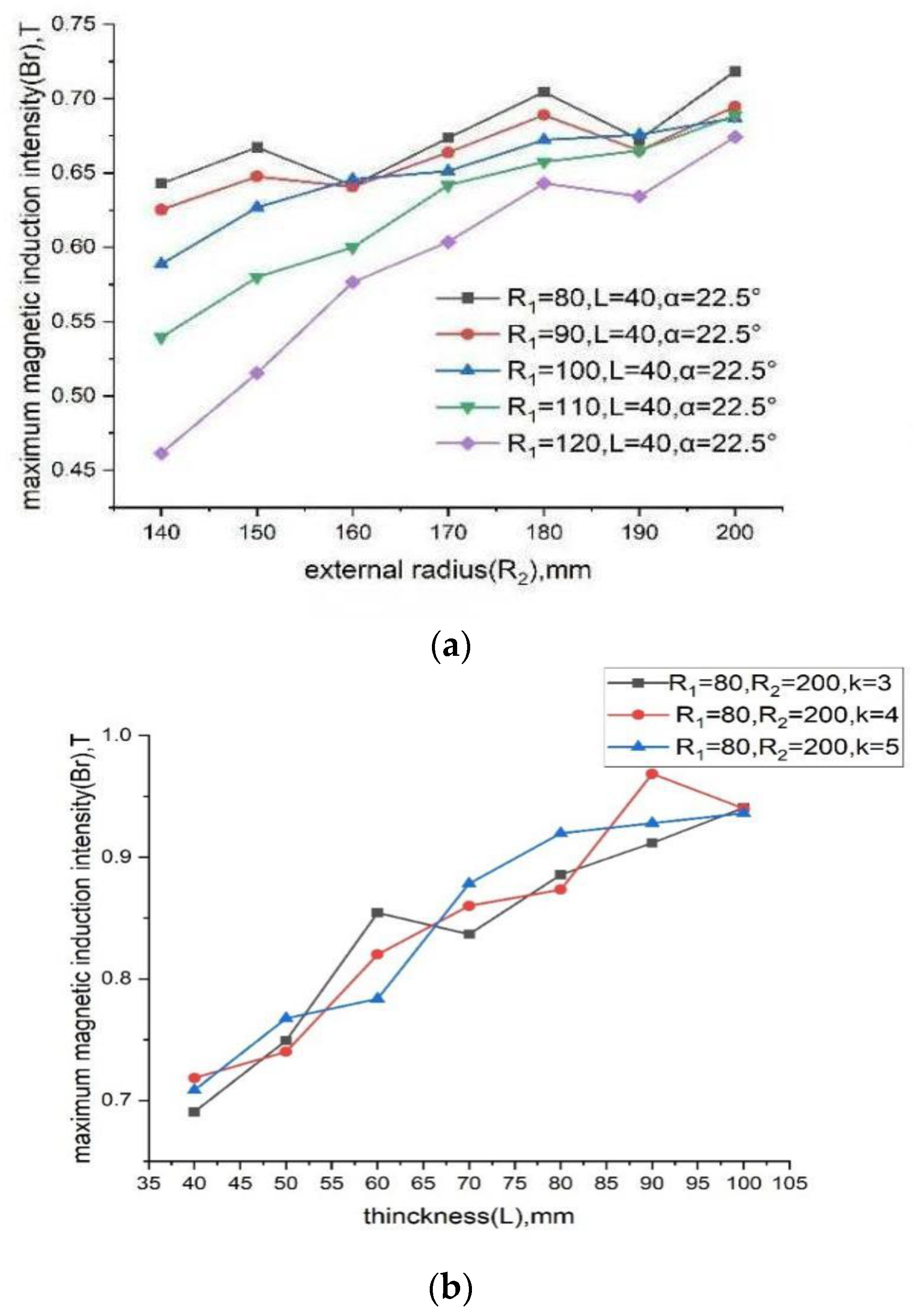
Based on the above-mentioned magnetic field models, the tangential magnetic induction intensity around the magnetic roller surface is associated with the external radius (R₂), internal radius (R₁), thickness (L), and sector angle (α) of a single permanent magnet. Using the above four parameters, we conduct numerical simulations for the Halbach magnetic rollers with a different external radius (R₂), internal radius (R₁), thickness (L), and sector angles (α) of a single permanent magnet, as well as the optimal parameters of external radius (R₂), internal radius (R₁), thickness (L), and sector angles (α) of the maximum tangential magnetic induction intensity around the magnetic roller surface (B_r). In this study, the air gap and soft iron are neglected.

To minimize the computational load, a cycle of three-dimensional models is employed. During the optimization, the external radius (R₂) of a single permanent magnet rises from 140 to 200 mm with a step of 10 mm, while the internal radius (R₁) increases from 80 to 120 mm with a step of 10 mm, with the remaining two parameters being constant (L = 40, α = 22.5°). The variations in Br with R₁ and R₂ are presented in Figure 5a. The dependent variable Br exhibits an elevation with an increasing R₁ and R₂ in general. It rises faster when the external radius is less than 180 m, and it later increases more slowly. There is a certain randomness. In more detail, the Halbach magnetic roller with a smaller internal radius and a larger external radius works with a higher magnetic strength.

The thickness of a single permanent magnet also has a certain effect on the surface magnetic field’s strength. From the above analysis, the Halbach magnetic roller’s external radius (R₂) equals 200 mm, and the Halbach magnetic roller has an internal radius (R₁) of 80 mm in the current investigation. Under this condition, the maximum intensity of magnetic induction outside the roller surface can reach the maximum. We still take α = 22.5°. Based on the three parameters, the effect of the thickness of a single permanent magnet on the magnetic field is investigated. During the optimization, the thickness of a single permanent magnet rises from 40 mm to 80 mm with the step of 10 mm.

Figure 5b shows the thickness of a single permanent magnet with four pole pairs having a significance on the tangential intensity of magnetic induction in the roller surface periphery as well. We can observe that k = 4 (α = 22.5°) is preferable. By contrast, the impact of R₁ and R₂ on Br is limited.

From the above analysis, it can be seen that the intensity of the magnetic field in the roller surface vicinity increases with increasing geometric size of a single permanent magnet on the presumption that the pair of magnetic poles is constant, while the influence on the surface is not particularly obvious when it increases to a certain degree on the whole. Thus, the four parameters, i.e., R₁, R₂, k, and L, need to be balanced in the optimal design of a concentric Halbach magnetic roller. For the current investigation, the parameter combination of R₁ = 200 mm, R₂ = 80 mm, L = 80 mm, and k = 4 (α = 22.5°) generates a good maximum Br of 0.8733T. Although the maximum value can be over 1 T when L is over 90 mm, the minimum value is below 0.2 T, which is not beneficial for the separation of larger scrap. In addition, the larger the structure, the more unfavorable the permanent magnet installation and manufacturing. Therefore, this combination of R₁ ∈ [160, 200], R₂ ∈ [80, 120], L ∈ [50, 80], and k = 4 (α = 22.5°) is adopted and applied in the following investigation.

3.2. Response Surface Analysis

3.2.1. Response Models

RSM model assessment was accomplished via the BBD in Design-Expert. To illustrate the output–input parameter correlations, the linear, quadratic, and bivariate interactions (2FI) were evaluated. The suggested optimal response models were chosen according to p < 0.05, where the significant regression coefficients approached 1. Table 5 details the fit statistics for the reduced cubic model, whose SD and R² (correlation coefficient) values were significant (p < 0.05). The adjusted R², which quantifies the variance around the model-explained mean, was below 0.20, an admissible model significance standard for the prediction in the absence of setbacks.

The RSM-BBD-derived response surface models exhibit quadratic functions of the actual input parameters as formulated in Equation (19). X₁, X₂, and X₃ represent the internal radius, external radius, and thickness of a single permanent magnet, respectively. The comparison of factor coefficients is conducive to unraveling the factors’ relative influence. Regarding the synergistic effect of terms, the positive and negative signs of respective peculiar coefficients serve as the determinants. Values of positive and negative coefficients in the model term indicate synergy and antagonism, respectively. Similarily, the terms of the interactive model discovered are (X₁X₂, X₁X₃, X₂X₃), with the three factors having no interaction. The model equation enables a response forecast for a predefined level of parameters as formulated in Equation (19):

$$\begin{array}{l}Y=-0.161343+0.006125X_1+0.001208X_2+0.004259X_3\\ +0.000031X_1{X}_2+0.000025X_1{X}_3-0.000058X_2{X}_3-0.000024X_1^2\\ -0.000024X_2^2+{1.8518510}^{-6}{X}_3^2\end{array}$$

(19)

3.2.2. Analysis of Variance (ANOVA)

According to the ANOVA outcomes in Table 1,

Table 2. Observed and estimated values for different levels of simulation.

Run	Factors			Response
	X1 (mm)	X2 (mm)	X3 (mm)	Br (T)
1	160	80	65	0.78
2	200	80	65	0.87
3	160	120	65	0.68
4	200	120	65	0.82
5	160	100	50	0.72
6	200	100	50	0.77
7	160	100	80	0.81
8	200	100	80	0.89
9	180	80	50	0.77
10	180	120	50	0.74
11	180	80	80	0.89
12	180	120	80	0.79
13	180	100	65	0.81
14	180	100	65	0.82
15	180	100	65	0.79

and

Table 3. Analysis of variance and statistical parameters for the regression model of the Br.

Source	Sum of Squares	DOF	Mean Square	F-Value	p-Value
Model	0.0468	9	0.0052	13.21	0.0055
$X_1$	0.0162	1	0.0162	41.19	0.0014
$X_2$	0.0098	1	0.0098	24.92	0.0041
$X_3$	0.0181	1	0.0181	45.89	0.0011
$X_1{X}_2$	0.0006	1	0.0006	1.59	0.2631
$X_1{X}_3$	0.0002	1	0.0002	0.5720	0.4835
$X_2{X}_3$	0.0012	1	0.0012	3.11	0.1379
$X_1^2$	0.0003	1	0.0003	0.8621	0.3958
$X_2^2$	0.0003	1	0.0003	0.8621	0.3958
$X_3^2$	$6.41\times {10}^{-7}$	1	$6.41\times {10}^{-7}$	0.0016	0.9694
Residual	0.0020	5	0.0004
Lack of Fit	0.0015	3	0.0005	2.14	0.3339
Pure Error	0.0005	2	0.0002
Cor Total	0.0487	14
R2 = 0.9596	Adj. R2 = 0.8870	Pre. R2 = 0.4860	C.V. = 2.49%	Adeq Precision = 12.5052

, the significant terms comprised linear, quadratic, and interactive terms with p < 0.05. F-values were employed for the significance assessment for relevant terms, while the regression model significance was presented by p-values [26,27]. The confidence level in the analysis of p probability was set at 95%. Despite p > 0.05 for several terms, which were thus insignificant, we included them in the final model to clarify their precision and predictability with R² > 0.95. The RSM coefficient of variation (CV < 10%) was computed, serving as the SD for the output parameter’s mean. Every term in the quadratic model was subjected to the significance evaluation according to the p-value [27]. Significance assessment on the model was accomplished through the Fisher’s F-test, and so was the importance assessment on every independent input term. The relevant calculation was accomplished by varying the mean square of the model by the residual error. A greater F-value indicated a more significant term of the model on the answer. The quadratic model was considered acceptable when p was <0.05. The ratio of the explained variation to the total variation R² was 0.9596, which is more than 0.9. That is to say, the relationship between the factor variables and response was significant, and the data can be well reflected by the model. The Adj. R² of 0.8870 was not in reasonable agreement with the Pre. 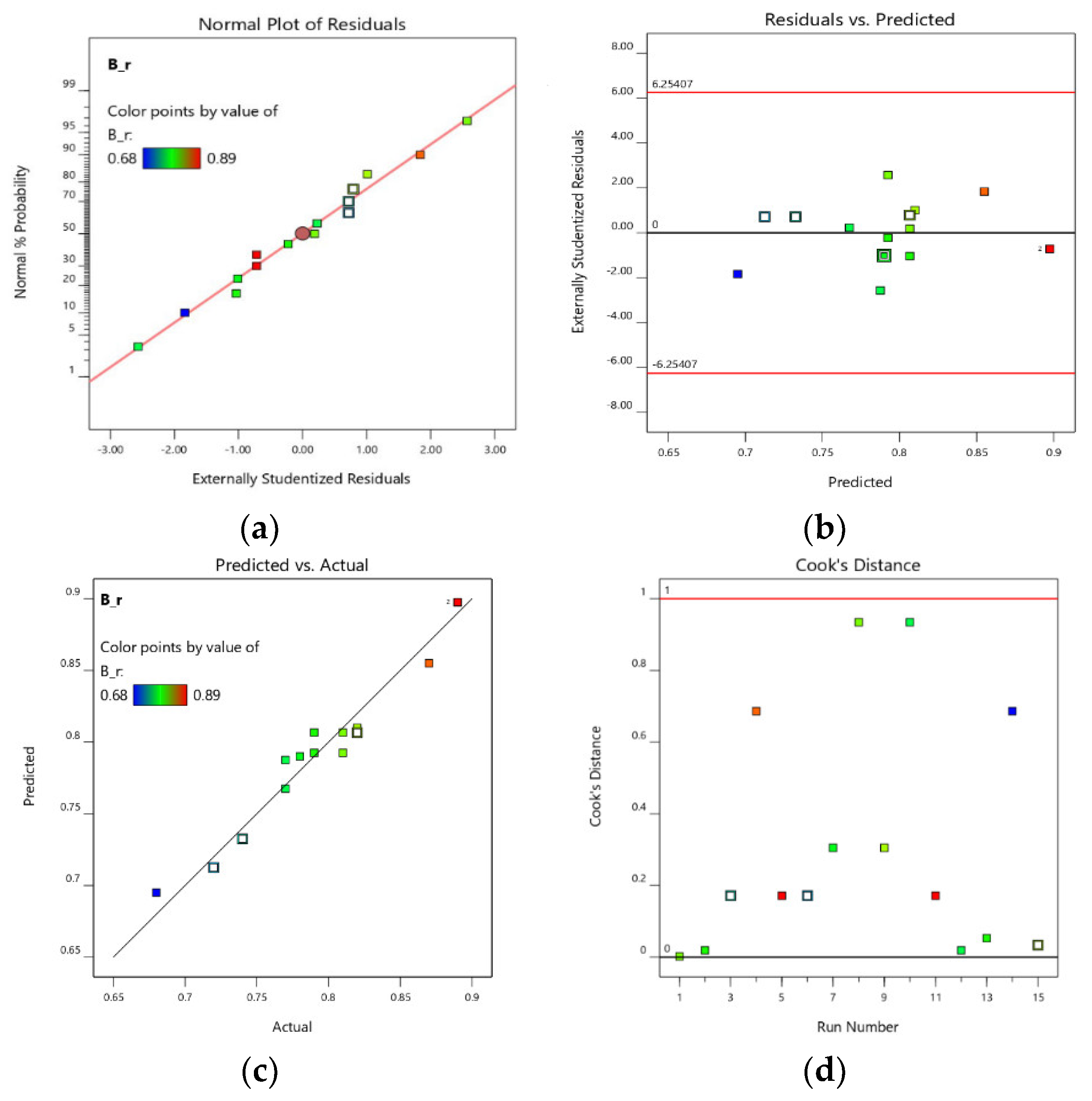R² of 0.4860, and the difference was more than 0.2, indicating that the fitting results were not in good agreement with the simulation results and the fitting reliability was low.

Figure 6 shows that the status of the residual is not normally distributed. The data of residuals 1, 2, 12, and 15 are inconsistent, so the data points are abnormal, which can be removed directly. The residual after removing the same data points is still normal. It is considered that the model is effective in general, while the fitting effect of the model is mediocre.

3.2.3. Response 3D Plots

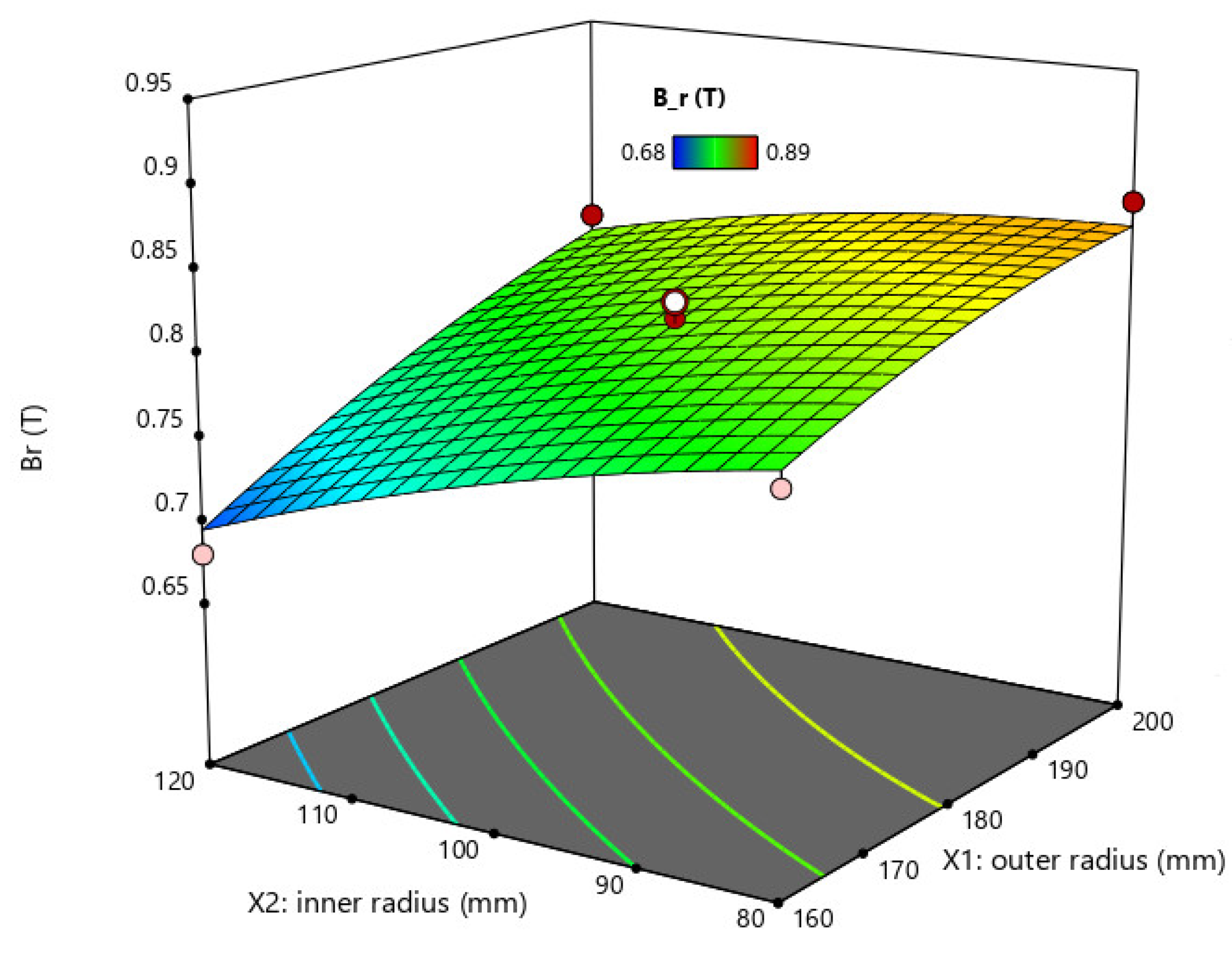
For the interactivity assessment of the input parameters plus the response, 3D response plots and other graphical approaches could be employed. For the maximum magnetic induction intensity around the surface of the roller (Y), the response variables are presented graphically against two individual design parameters (X₁X₂) in Figure 7. The model-based generation of surface plots was performed through the alteration of two arbitrary variables (internal radius, external radius, or thickness of a single permanent magnet) inside the design space, during which the remaining individual component constant was maintained at its midpoint. Graphically, as shown in Figure 7, the response surface was arc-shaped, with the optimal zone for maximum magnetic induction intensity around the surface of the roller at the high–low X₁X₂ levels. Based on the plateau-shaped response surface in Figure 7, the optimal zone for the response was at the extreme X₁X₂ levels. In the 3D response plots, the visible peaks suggest that the suitable conditions enabling the performance of response variables to be optimal were inside the horizon or border of the design space. As shown in the graphs, the internal radius and external radius of a single permanent magnet had a substantial effect on the maximum magnetic induction intensity around the surface of the roller (Figure 7).

3.3. Comparing the Results of Kernel Functions of SVR

In our simulation study, we compare the four kernels (linear, sigmoid, polynomial, and radial basis kernel functions), as introduced in Section 3. These compared kernels are implemented in MATLAB R2022a. A regression support vector machine model is created using FITRSVM.

The superiorities and deficiencies of the training model are assessed by such indices as the RMSE, accuracy, and MSCC. A lower RMSE, which is the variance, indicates better SVM stability. A higher accuracy represents a better result. A higher MSCC, which refers to the linear correlation between experimental and predicted value variances, indicates a superior model.

Since the emphasis of the present work is laid on the type selection for the kernel function, the method of a predefined constant value is employed for the SVM-associated penalty parameter C, as well as the RBF parameter g. Specifically, the RBF and the hybrid kernel function parameter C comprising RBF are assigned as 100 experientially, while the value of parameter g is assigned as 0.1. For other kernel functions and hybrid kernel functions without a radial basis, the parameter C setting is 1.72.

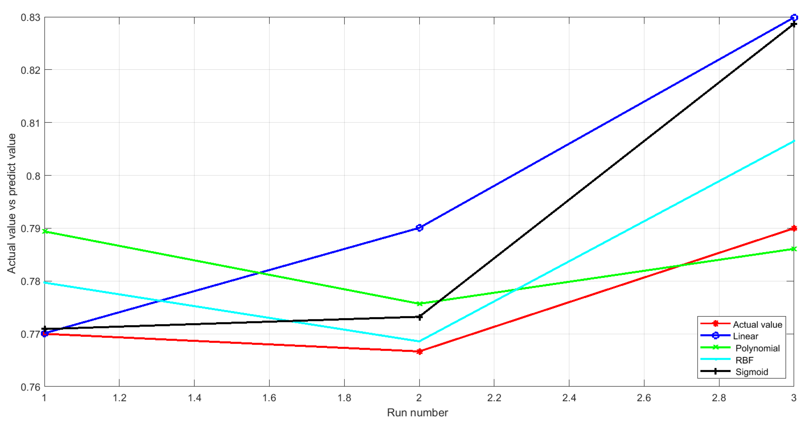
Figure 8 presents the comparison of four kernels regression results. The linear regression result exhibits a 0.0026 RMSE, a 99.9340% accuracy, and a 0.97228 MSCC. The polynomial regression result exhibits a 0.0133 RMSE, a 99.9824% accuracy, and a 0.78099 MSCC. Based on the RBF regression, the RMSE is 0.0162, the accuracy is 99.9738%, and the MSCC is 0.9894. According to the sigmoid regression result, the RMSE is 0.0251, the accuracy is 99.9368%, and the MSCC is 0.97696.

Table 4. Simulation statistics of roller performance for various kernel functions.

Selected Kernel Function Types	Accuracy	RMSE	MSCC
Linear	99.9340%	0.0026	0.97228
Poly	99.9824%	0.0133	0.78099
RBF	99.9738%	0.0162	0.9894
Sigmoid	99.9368%	0.0251	0.97696

summarizes all the data. Obviously, the precision of the investigated kernel functions is high. The RMSE of RBF is highest, far more than 0.9596 of RSM. To sum up, RBF generates greater regression results.

3.4. Optimization Using SSA

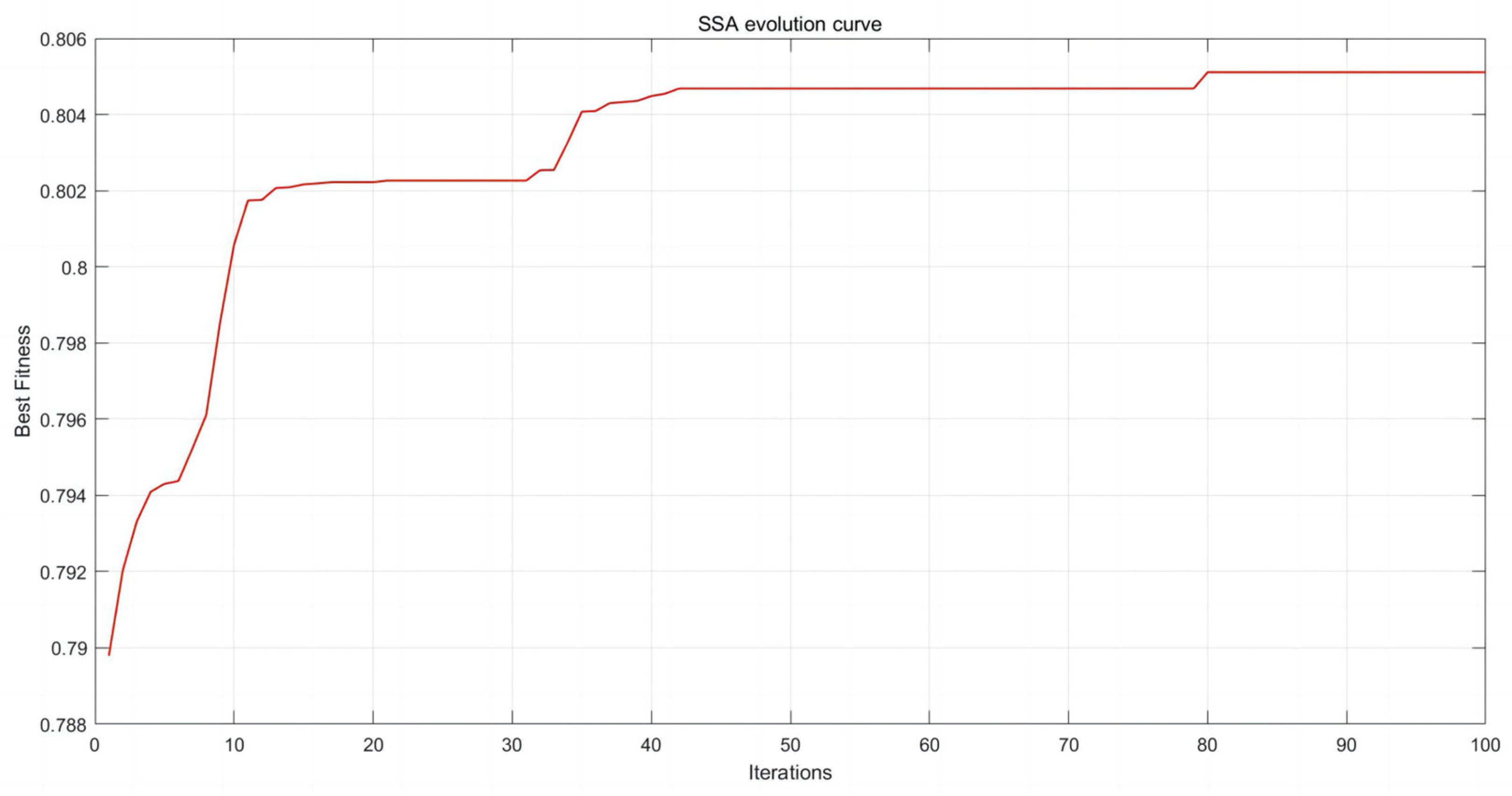
The model established according to the above RBF is used as the fitness function of the SSA. The use of the SSA to find the magnetic roller indicates the maximum magnetic induction intensity setting Max_iter = 100, pop = 50. As shown in Figure 9, with the increasing evolutionary number, the best and average values of fitness for the population both present a tortuous upward trend. After 20 iterations, both the best and average values of fitness for the population tend to be stable. When the best and average values of fitness are identical for the population, the residual value is obtained. For the corresponding objective function of the transmission algorithm, its optimal solution (predicted value) is Y = 0.9061, more than the 0.89 of RMS, and the optimized variable values X are 193. 0740, 85.4563, and 80.4532.

4. Model Validation

The design parameters of the roller, which correspond to the global optimal solution, and the structural parameters are modified, are shown in

Table 5. The structural parameters of magnetic roller.

Items	Value
External radius, R2 (mm)	194
Internal radius, R1 (mm)	85
Thickness, L (mm)	80
Radians of the magnetic block, $\alpha$ (°)	22.5
The number of magnets, N	16
Number of pole pairs, k	4
Magnet remanence, Br (T)	1.4
Coercivity, Hc (A/m)	900,000
Relative permeability	1.24

.

This study investigates the radial distribution of the magnetic field intensity of the Halbach magnetic roller. The effective working area of interest is located at a distance of 20 mm around the surface of the permanent magnet. Simulations of the distances of 5 mm, 10 mm, 15 mm, and 20 mm from the surface of the permanent magnet are conducted (see Figure 10). The results demonstrate that the magnetic field intensity of the magnetic roller varies periodically along the radial direction. The closer the distance is to the surface of the magnetic roller, the stronger the magnetic induction intensity is, and it peaks to 0.9416 T at 5 mm away from the surface of the magnetic roller. The minimum range of the magnetic induction intensity is less than 10%. The magnetic induction intensity of the rest region within 20 mm is more than 0.4 T. The results would be better if the back-iron and magnetic gap were considered in our investigation.

5. Conclusions

In this study, to optimize the numerical simulation results by using machine learning for the first time and to improve the generalization capability of SVR, a novel strategy is proposed, in which the four common kernel functions are compared. Then, the SSA is employed to optimize the structural parameters of the Halbach magnetic roller. The process solves both the kernel function selection and parameter selection problems. Through the case study, the following conclusions are obtained.

• The results show that machine learning for magnetic roller optimization is feasible.
• The methodology of comparing four kernel functions improves the accuracy of prediction compared with the single kernel SVR model.
• More accurate model selection results are obtained by utilizing the SSA for structural parameter optimization of the Halbach magnetic roller.

In conclusion, our strategy provides an alternative without establishing a large number of finite element models.

The process successfully improves the prediction of intensity over the roller surface of the Halbach magnetic roller using machine learning, providing a valuable reference for Halbach magnetic roller optimization. However, our study still has some limitations. Firstly, numerical simulation data are the input to the model in our work. Secondly, the samples of SVR are limited, and thus, a linear fitting error may exist. Therefore, our future work is presented as follows: (1) adding more samples into the training of the model; (2) developing more efficient optimization algorithms to compare, and then confirming the optimal structural parameters of the Halbach magnetic roller; (3) adding deep learning algorithms into our numerical simulation models, and (4) validating models by manufacturing a virtual prototype.

References

1. Available online: https://baijiahao.baidu.com/s?id=1728550320642512403&wfr=spider&for=pc (accessed on 28 March 2022).
2. Tang, Y.; Zhang, Q.; Li, Y.; Wang, G.; Li, Y. Recycling mechanisms and policy suggestions for spent electric vehicles’ power battery—A case of Beijing. J. Clean. Prod. 2018, 186, 388–406. [Google Scholar] [CrossRef]
3. Zhou, F.; Wang, X.; Lin, Y.; He, Y.; Zhou, L. Strategic part prioritization for quality improvement practice using a hybrid MCDM framework: A case application in an auto factory. Sustainability 2016, 8, 559. [Google Scholar] [CrossRef]
4. Bulach, W.; Schuler, D.; Sellin, G.; Elwert, T.; Schmid, D.; Goldmann, D.; Buchert, M.; Kammer, U. Electric vehicle recycling 2020: Key component power electronics. Waste Manag. Res. J. Int. Solid Waste Public Clean. Assoc. Iswa. 2018, 36, 311. [Google Scholar] [CrossRef] [PubMed]
5. Phuc, P.N.K.; Yu, V.F.; Tsao, Y.C. Optimizing fuzzy reverse supply chain for end-of-life vehicles. Comput. Ind. Eng. 2018, 113, 757–765. [Google Scholar] [CrossRef]
6. Zhou, F.; Wang, X.; Lin, Y.; He, Y.; Zhou, L. Supplier portfolio of key outsourcing parts selection using a two-stage decision-making framework for Chinese domestic auto-maker. Comput. Ind. Eng. 2019, 128, 559–575. [Google Scholar] [CrossRef]
7. Andersson, M.; Ljunggren, S.M.; Sanden, B.A. Are scarce metals in cars functionally recycled? Waste Manag. 2017, 60, 407–416. [Google Scholar] [CrossRef]
8. Sverdrup, H.U.; Ragnarsdottir, K.V.; Koca, D. An assessment of metal supply sustainability as an input to policy: Security of supply extraction rates, stocks-in-use, recycling, and risk of scarcity. J. Clean. Prod. 2017, 140, 359–372. [Google Scholar] [CrossRef]
9. Cui, J.; Forssberg, E. Mechanical recycling of waste electric and electronic equipment: A review. J. Hazard. Mater. 2003, 99, 243–263. [Google Scholar] [CrossRef]
10. Ruan, J.; Zhu, X.; Qian, Y.; Hu, J. A new strain for recovering precious metals from waste printed circuit boards. Waste Manag. 2014, 34, 901–907. [Google Scholar] [CrossRef]
11. Weichao, Y.; Zhu, Z.; Chang, Z.; Zhao, L.; Dai, Z.; Zhang, K.; Ning, F.; Zhang, G.; Hou, Z.; Wang, M.; et al. Development of an eddy-current separation equipment with high gradient superconducting magnet. IEEE Trans. Appl. Supercond. 2014, 25, 1–4. [Google Scholar] [CrossRef]
12. Dholu, N.; Nagel, J.R.; Cohrs, D.; Rajamani, R.k. Eddy current separation of nonferrous metals using a variable-frequency electromagnet. KONA Powder Part. J. 2017, 34, 241–247. [Google Scholar] [CrossRef]
13. Lungu, M.; Neculae, A. Eddy current separation of small nonferrous particles using a complementary air-water method. Separ. Sci. Technol. 2017, 53, 126–135. [Google Scholar] [CrossRef]
14. Ruan, J.; Dong, L.; Zheng, T.; Huang, M.; Xu, Z. Key factors of eddy current separation for recovering aluminum from crushed e-waste. Waste Manag. 2017, 60, 84–90. [Google Scholar] [CrossRef] [PubMed]
15. Ouili, M.; Mehasni, R.; Feliachi, M.; Belounis, A.; Latreche, M.E.H. A simultaneous separation of magnetic and conductive particles in a designed permanent magnet drum separator. Int. J. Appl. Electromagn. Mech. 2019, 61, 137–155. [Google Scholar] [CrossRef]
16. Merahi, A.; Hader, A.; Benatia, M.B.; Medles, K.; Dascalescu, L. A new approach for the numerical analysis of an eddy current separator to recover non-ferrous metals from wastes. Int. J. Environ. Stud. 2020, 77, 749–766. [Google Scholar] [CrossRef]
17. Amir, M.; Karim, M.; Mourad, B.B.; Amar, T. Design and development of a low cost technique for sorting household wastes using eddy current separation process. Int. J. Environ. Stud. 2016, 73, 203–213. [Google Scholar] [CrossRef]
18. Fenercioglu, A.; Barutcu, H. Performance determination of novel design eddy current separator for recycling of non-ferrous metal particles. Jpn. Mag. 2016, 21, 635–643. [Google Scholar] [CrossRef]
19. Nagel, J.R. An analytic model for eddy current separation. Miner. Eng. 2018, 127, 277–285. [Google Scholar] [CrossRef]
20. Xue, J.; Shen, B. A novel swarm intelligence optimization approach: Sparrow search algorithm. Syst. Sci. Control Eng. 2020, 8, 22–34. [Google Scholar] [CrossRef]
21. Al-Sharif, L.; Taifour, S.; Kilani, M. Simulation and verification of the axial force of a linear permanent magnet synchronous actuator. Int. J. Appl. Electrom. 2010, 32, 249–265. [Google Scholar] [CrossRef]
22. Wu, Y.C.; Lee, Y.S.; Yang, J.C. Robust and efficient multiclass SVM models for phrase pattern recognition. Pattern Recognit. 2008, 41, 2874–2889. [Google Scholar] [CrossRef]
23. Hast, L.Y.; Liner, D.X.; Wang, T.Y.; Wang, P. Research on SVM Based Diagnosis System for Oil Tubing. Key Eng. Mater. 2016, 693, 1405–1411. [Google Scholar]
24. Samantaray, S.; Sahoo, A. Prediction of suspended sediment concentration using hybrid SVM-WOA approaches. Geocarto Int. 2021, 37, 5609–5635. [Google Scholar] [CrossRef]
25. Samantaray, S.; Sahoo, A.; Ghose, D.K. Assessment of Sediment Load Concentration Using SVM, SVM-FFA and PSR-SVM-FFA in Arid Watershed, India: A Case Study. KSCE J. Civ. Eng. 2020, 24, 1944–1957. [Google Scholar] [CrossRef]
26. Igwegbe, C.A.; Mohmmadi, L.; Ahmadi, S.; Rahdar, A.; Khadkhodaiy, D.; Dehghani, R.; Rahdar, S. Modeling of adsorption of methylene blue dye on Ho-CaWO4 nanoparticles using response surface methodology (RSM) and artificial neural network (ANN) techniques. MethodsX 2019, 6, 1779–1797. [Google Scholar] [CrossRef]
27. Adeogun, A.I.; Bhagawati, P.B.; Shivayogimath, C.B. Pollutants removals and energy consumption in electrochemical cell for pulping processes wastewater treatment: Artificial neural network, response surface methodology and kinetic studies. J. Environ. Manag. 2021, 281, 111897. [Google Scholar] [CrossRef]
Figure 1. Halbach magnetic roller structure. (a) The schematic diagram of the cylindrical magnetic roller configuration. (b) Equivalent current model of radial magnetization in a single permanent magnet.
Sustainability 15 13451 g001
Figure 2. The schematic diagram of the SVR.
Sustainability 15 13451 g002
Figure 3. Insensitive loss function.
Sustainability 15 13451 g003
Figure 4. The scheme of Halbach magnetic roller optimization.
Sustainability 15 13451 g004
Figure 5. Illustration of impact of geometrical parameters on the maximum magnetic induction intensity: (a) performance variations of Halbach magnetic roller with internal radius and external radius of a single permanent magnet; (b) performance variations of Halbach magnetic roller with thickness of a single permanent magnet and the number of pole pairs.
Sustainability 15 13451 g005
Figure 6. Residual plots: (a) plot of normal probability distribution of residuals; (b) distribution of residual and predicted values; (c) RSM−BBD predicted vs. actual value of Br; (d) residuals.
Sustainability 15 13451 g006
Figure 7. 3D contour plot of maximum magnetic intensity outside the surface of the roller.
Sustainability 15 13451 g007
Figure 8. Plot of actual value vs. predicted value.
Sustainability 15 13451 g008
Figure 9. SSA evolution curve.
Sustainability 15 13451 g009
Figure 10. Comparison of magnetic induction intensity at different distances from magnetic roller surface.
Sustainability 15 13451 g010