Article

Simulation of Surface Settlement Induced by Parallel Mechanised Tunnelling

1
Department of Civil Engineering, Faculty of Engineering, University of Malaya, Kuala Lumpur 50603, Malaysia
2
School of Civil and Environmental Engineering, University of Technology Sydney, Sydney, NSW 2007, Australia
3
Department of Civil Engineering, Faculty of Engineering, Universiti Malaysia Sarawak (UNIMAS), Kota Samarahan 94300, Sarawak, Malaysia
*
Authors to whom correspondence should be addressed.
Sustainability 2023, 15(17), 13265; https://doi.org/10.3390/su151713265
Submission received: 18 July 2023 / Revised: 17 August 2023 / Accepted: 31 August 2023 / Published: 4 September 2023
(This article belongs to the Special Issue Advances in Rock Mechanics and Geotechnical Engineering)

Abstract

:
Mechanised tunnelling is extensively utilised for twin tunnel construction, particularly in urban areas. A common challenge encountered during this construction method is the occurrence of surface settlement (SS) induced by tunnelling activities. The integrity of nearby structures can be compromised by SS, making it imperative to accurately quantify and mitigate this phenomenon. Several methods for determining SS exist, including empirical formulas and laboratory studies. However, these methods are often constrained by specific soil types and are time-consuming. Moreover, crucial parameters such as tunnel operational factors and construction stages are often omitted from empirical formulas. Given these limitations, this paper aims to address these challenges by employing 3D numerical analysis to simulate tunnelling-induced SS in twin tunnels. This approach takes into account tunnel geometry, construction sequencing, soil properties, and tunnelling operational factors. By incorporating data from in-situ and laboratory tests conducted on the ground, engineering soil parameters are established as inputs for the numerical analysis. The simulated SS results obtained from the 3D numerical analysis are compared with field measurements of SS taken from available ground surface settlement markers. The transverse SS pattern derived from the numerical analysis closely mirrors the field measurements. Additionally, SS values above the first and second tunnels are compared with field measurements, resulting in coefficient of determination (R2) values of 0.94 and 0.96, respectively. The utilisation of the 3D numerical modelling approach enables the customizable mitigation strategies for managing the SS with project-specific parameters such as tunnel geometry, geotechnical engineering factors, and tunnelling operational variables. This will help plan and construct more sustainable tunnels with minimal effects on the ground and residential areas.

1. Introduction

Tunnelling is one of the most significant transport solutions where the overlying population does not need to be displaced. With the advancement of current technologies, mechanised excavations to construct underground spaces such as tunnels have become popular. Although mechanised tunnel excavations have been widely used all around the world, considerable safety considerations during construction need to be ensured. Several problems can be encountered during tunnel excavations, such as tunnel face instability, excessive wear of the cutter head, and excessive surface settlement (SS) [1,2]. Among them, SS induced by mechanised tunnelling is still one of the common issues in tunnel construction [3,4]. The excessive SS during and after tunnelling projects has an adverse impact on the existing structures. Therefore, it is important to estimate the settlements caused by the tunnelling to minimise the effects on the existing structures. Several methods can be used to estimate the SS due to tunnelling, which is empirical or semi-empirical, laboratory-based, and numerical analysis. One of the pioneer empirical formulas to determine the SS due to tunnelling was proposed by Peck [5], which shows that the volume loss is from the radial deformations along the tunnel perimeter directly linked to the SS. Based on the field observations on the site and the simplification of the equation proposed by Litwiniszyn [6], Peck [5] suggested Equation (1) to predict SS induced by tunnelling for soft clay. The settlement in this equation is calculated based on the pattern of SS caused by loss of ground and approximated by a Gaussian probability curve.
S = S m a x e x 2 2 i 2
where S is the surface settlement in the transverse section at a specific distance, x is the distance from the centreline of the tunnel, and i is the point of inflection (settlement through). In this way, the maximum SS can be defined using Equation (2):
S m a x = V s   2   x   π   x   i
where Vs is the volume loss of the soil (m3/m), and can be expressed by Equation (3):
V s = V o l u m e   L o s s   ( V L ) ( % ) 100 ( π   D 2 4 )
The main inputs for the calculation of the maximum SS are affected by volume loss of the soil (VL) and settlement trough. These volume losses are affected by the type of ground, tunnel geometry, and ground condition [7,8]. Hence, many researchers have carried out their investigations into different types of ground conditions with various ranges of VL, as summarised in Table 1. In addition, several researchers have also proposed various i equations for different ground conditions, as presented in Table 2.
According to Table 2, VL and i have a wide range of values, which can be due to different methods of tunnel construction and ground conditions. It can also be seen that most studies are carried out for clay material. In addition, no tunnelling operational parameter is included in the previous empirical formulas. Loganathan and Poulos [16] proposed a semi-empirical equation (i.e., Equation (4)), which is based on the gap parameter proposed by Lee et al. [19] and the exponential function to model the nonlinear ground movement. This formula has been checked with the five case studies. From the findings, four tunnels that were constructed in stiff clay showed good agreement; however, soft clay depicted a much lower estimation of the ground loss. Nevertheless, the method proposed by Loganathan and Poulos [16] is limited to clay and based on an elastic solution.
ε x y = 4 g R + g 2 4 R 2   e 1.38 x 2 ( Z + R ) 2 + 0.69 z 2 Z 2
where R′ is the radius of tunnel, Z is the tunnel depth below ground level, z is the depth of the point, g is the gap parameter, and εxy is the equivalent ground loss component at the tunnel soil interface due to the ground movements at point x, z.
Aside from the empirical and semi-empirical equations, 2D finite element analysis has been widely used to determine SS induced by tunnelling. Some of these 2D simplified techniques are the contraction method by Vermeer and Brinkgreve [20], the stress reduction method by Addenbrooke et al. [21], and the modified grout pressure method by Surarak [22]. The contraction method of the analysis works with the introduction of the correction factor (which represents the value of reduction and excavated area) as a predefined uniform radial inward strain. However, this assumption may not reflect the actual field displacement because, based on the centrifuge modelling study carried out by Mair [23], the finding shows that little ground displacement happens at the tunnel invert. In addition, the stress reduction method uses an “unloading factor” to stimulate the 3D tunnelling effects in the 2D numerical model, but this method requires trial-and-error on the unloading factor to calculate/determine the SS induced by tunnelling. Additionally, the modified grout pressure method [22] is the method that considers the tunnel operation parameter for the analysis. Although this method can include the operational parameters (face pressure and grout pressure), it does not consider the 3D mechanised tunnelling sequence in the analysis. Every stage of the mechanised tunnelling construction influences the ground SS. The stages of the tunnelling such as excavation using face pressure, advancement of the tunnelling machine, installation of the lining, injection of the tail void grout, and hardening of the grout, affect the surrounding soil area [24,25]. Apart from that, the type of soil model used in the numerical analysis is important; therefore, proper in-situ and laboratory data interpretation is required to stimulate the closest possible ground conditions at the site. In 3D numerical analysis, the tunnelling construction can cause SS at different stages of the construction. Mathew and Lehane [26] deduced the inconsistency of the calculations using volumetric contraction in comparison with field measured settlements due to the complexities of the actual tunnelling procedures. In comparison with a single tunnel, twin tunnels are more complex and more difficult to analyse as more parameters e.g., the spacing between two tunnel and different tunnelling operational parameters are required to consider in the analyses.
Most studies [3,27] investigated these issues for single tunnels; however, limited studies are available for twin tunnels using earth pressure balance (EPB) shield machines. In the recent numerical tunnelling analysis carried out by Islam and Iskander [28], the effect of geometric parameters and construction sequence on the SS was investigated using MIDAS GTS NX software 2021 (v1.1). However, this case study is not for parallel twin tunnelling and the outputs were not compared with the field measurements. The 3D numerical model is not limited to certain types of ground in comparison with the empirical and semi-empirical methods. In addition, the 3D numerical model requires a shorter period of time to determine the SS than the laboratory works. The 2D numerical methods (contraction and stress reduction methods) do not consider operational parameters in the analysis, whereas modified grout pressure does not consider the construction stages of the tunnelling works such as the advancement of the tunnelling machine. The consideration of important factors affecting the SS due to tunnelling in the analysis is crucial to providing the closest possible results with the actual measurements.
In light of the above discussion, this study considers the holistic approach of 3D modelling shield tunnelling works in the finite element by incorporating the sequence of mechanised tunnel construction. This sequence includes different stages such as excavation, machine advancement, lining installation, grouting, and hardening. Additionally, most previous research, especially empirical formulas, is solely applicable for a single tunnel. Many existing empirical formulas are tailored to single tunnel scenarios and do not account for modern tunnelling machine processes. This work extends the analysis to twin tunnels constructed using mechanised tunnelling, which presents a more complex scenario due to the interactions between adjacent tunnels. The utilisation of the 3D numerical modelling approach provides a sustainable solution for tailoring mitigation strategies to effectively manage SS while accounting for project-specific parameters such as tunnel geometry, geotechnical engineering factors, and tunnelling operational variables. The 3D numerical model approach empowers the customization of SS mitigation strategies. This customization ensures not only the effectiveness of the mitigation strategies but also the adherence to sustainability principles by minimizing adverse impacts on the environment and adjacent structures. By identifying potential SS issues at various construction stages through early estimation, timely adjustments and proactive measures can be implemented, thereby mitigating risks, and reducing the likelihood of detrimental effects on the surroundings.

2. Field Measurement and Input Parameter for Numerical Analysis

The Mass Rapid Transit (MRT) project is located in the Klang Valley, Malaysia, which comprises of total distance track of 52.2 km including the elevated works, underground works and one deport of the MRT system with the purpose of public transport for the citizens. In this project, the total distance of the twin tunnels is 13.5 km. The twin tunnel is two tunnels that can be arranged into four configurations: parallel, stacked, perpendicular crossing, and offset arrangements. The tracked alignment, a combination of parallel and stacked underground tunnels, is from Jalan Ipoh to Bandar Malaysia. Only parallel tunnelling is used for this study, as limited information is only available for stacked underground tunnels. The tunnel is traversed through limestone, granite, alluvium, and the Kenny Hill formation, as shown in Figure 1.
The project used mechanised tunnelling for tunnel excavation, including EPB and variable density tunnelling (VDT) machines with 6.7 m diameter for different ground conditions. VDT is the new mechanised tunnelling machine that was developed to mitigate the risk of blowouts and sinkholes in variable and mixed ground conditions. Whereas EPB was selected for the homogenous and cohesive soils. It uses the excavated material to stabilise the tunnel face with constant pressure. The selected section for the 3D numerical analysis is located between the alluvium and Kenny Hill. Several early geologists [29,30] have used diluvium as a term to describe “alluvium-like” materials comprised of sands, gravels, boulders, and clays on the hard rock in all landscape positions. The alluvium is modern sediments deposited into the ground as a result of recent river activity [31]. Since this soil material is deposited by the river, it can be anticipated that the ground is soft for the alluvium. Furthermore, the Kenny Hill formation in Kuala Lumpur has a thickness of 1200–1500 m of clastic sedimentary rocks and is located in the west and south [32]. It can be stated that this formation is for weathered rock and residual soil [33]; therefore, this formation is anticipated as a firm and hard material. This project encounters two different soil hardness materials: soft (alluvium) and hard (Kenny Hill).
Figure 1. The geological formation and location of the twin tunnels investigated in this research [34].
Sustainability 15 13265 g001

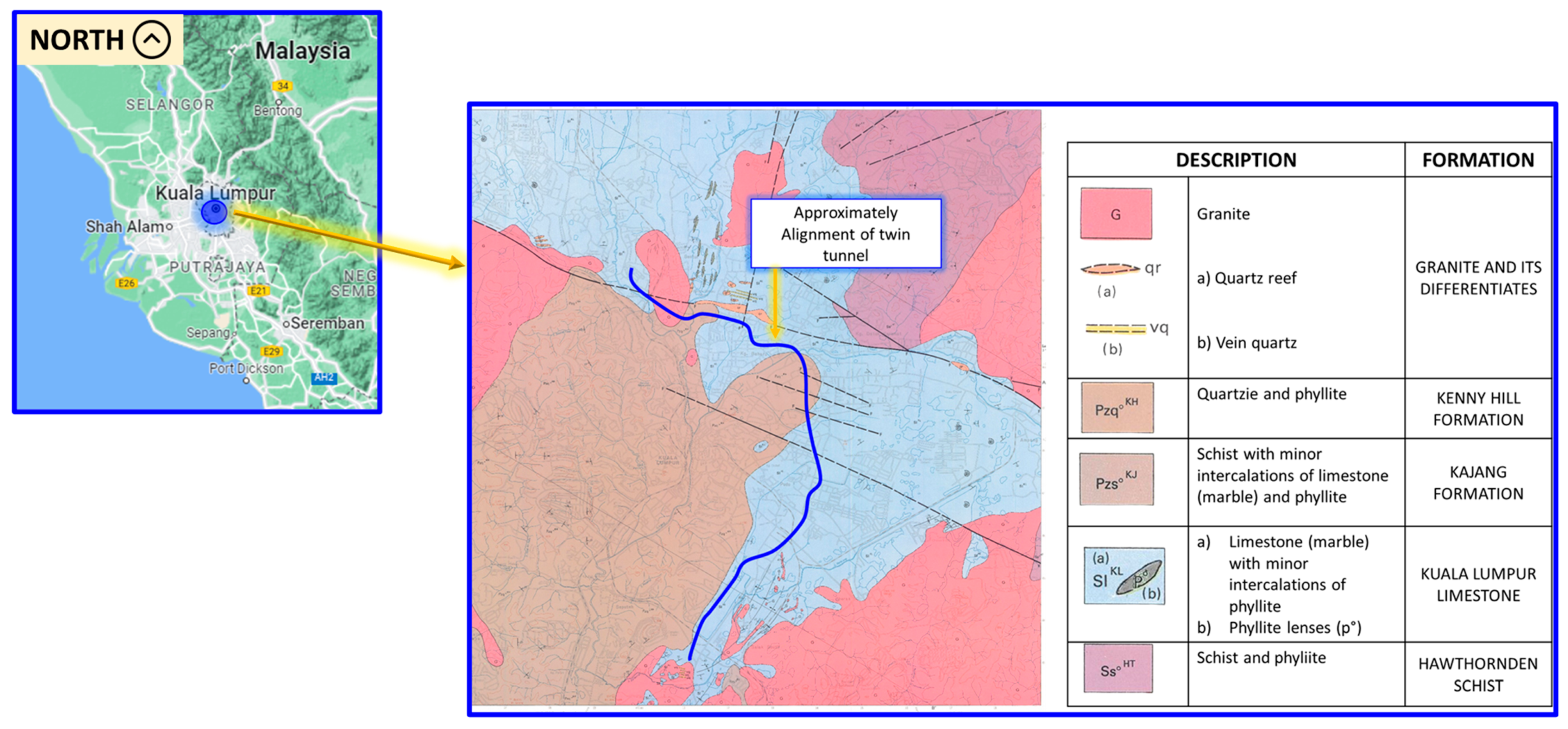
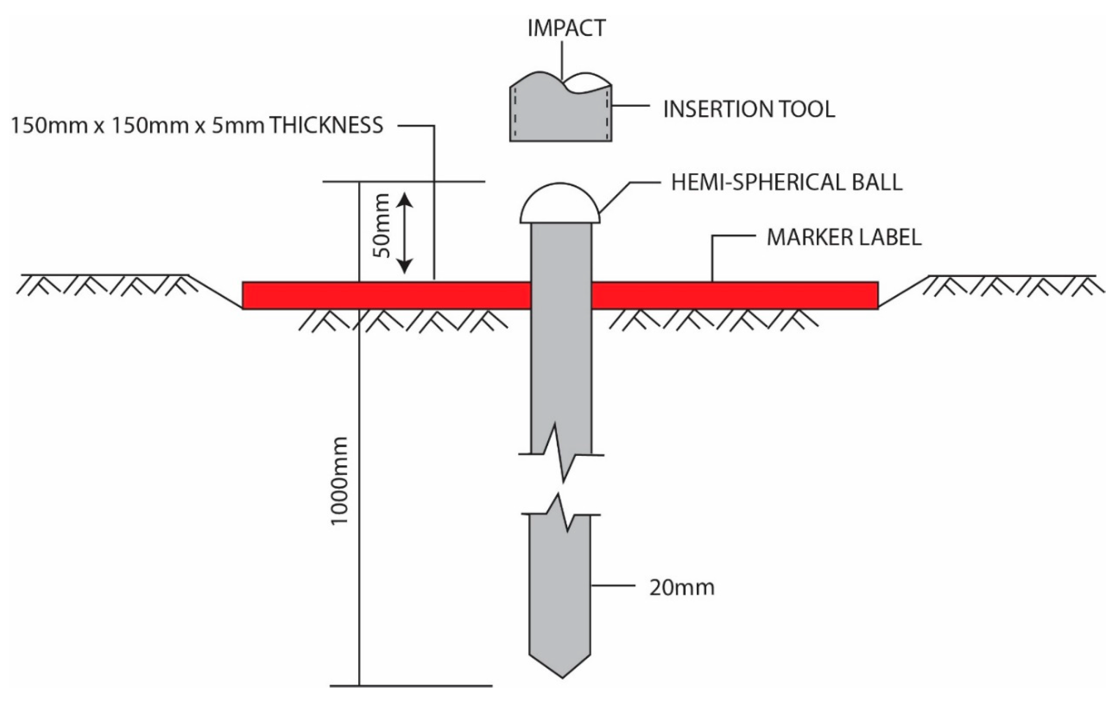
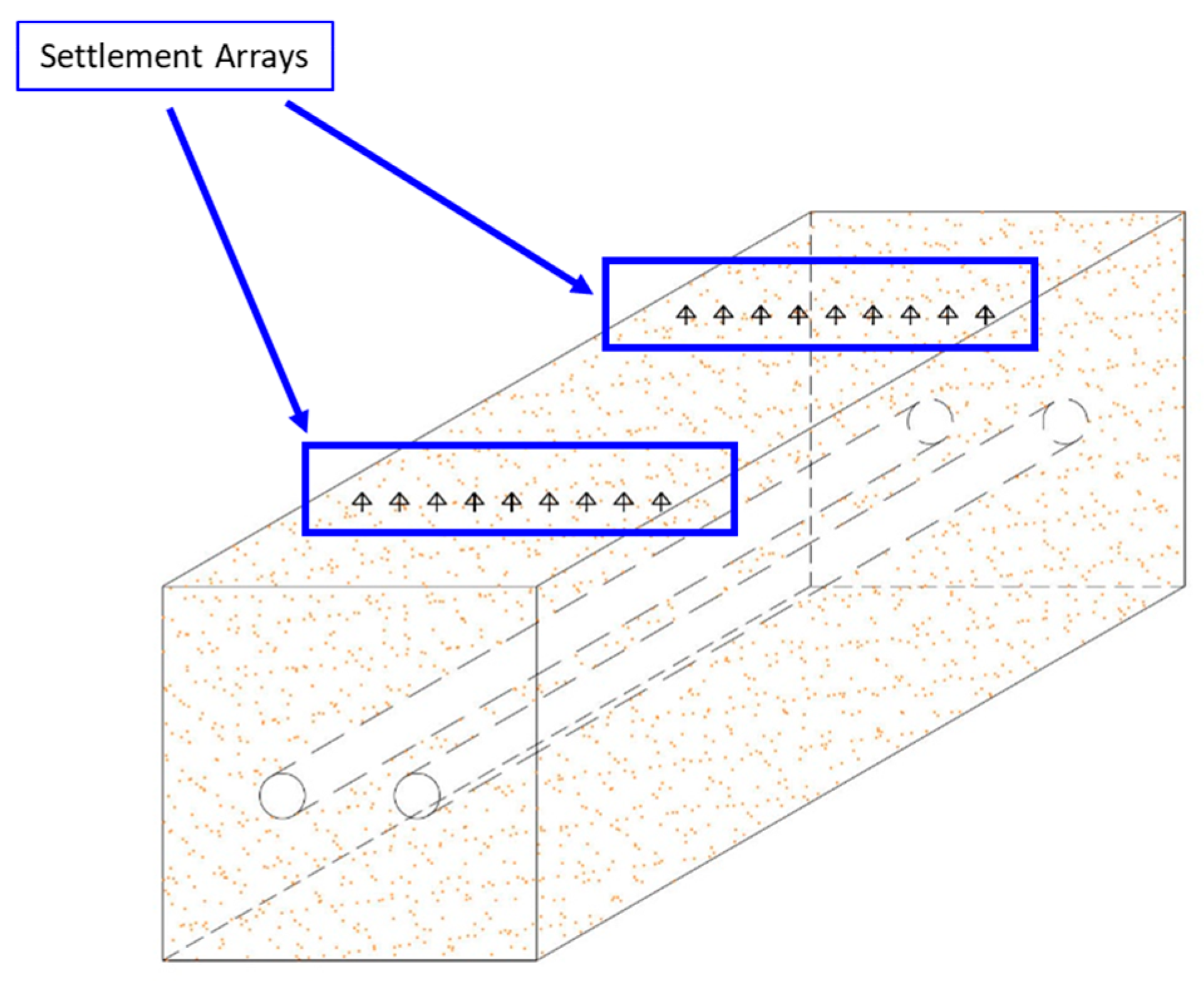
2.1. Field Measurement of SS

Throughout the chainage of the tunnelling, the overburden of the soil at the tunnel crown is in the range of 6 m to 42 m. For the back analysis of the SS due to tunnelling, five cross sections of the tunnel that traverse through the soil with a sufficient array of ground settlement markers were selected. In this project, the SS values were measured using a total station from the ground settlement marker as shown in Figure 2.
The ground settlement marker for this project is an instrument with a steel rod length of 0.95 m embedded in the soil that is covered by a steel plate of 150 mm by 150 mm, which acts as a marker label to ease the identification of the location of the markers. The protrusion of a 0.05 m steel rod above the marker label was used to measure the level of the change. The reduced levels of the tops of the rods of settlement markers based on the nearest benchmark (BM) or temporary BM were measured prior to the commencement of the tunnelling works. The baseline readings were set after taking readings for several days before the commencement of the tunnelling works. The settlement was calculated by taking the change in the reduced level of the top of the rod relative to the base readings and previous readings. In general, the readings of the settlement markers were taken once per day during the construction period of the tunnelling. To evaluate the settlement from the field data, the settlement values were collected when both tunnels had passed by the settlement array, as illustrated in Figure 3, and only the final readings were collected as the SS. There are approximately 304 subsurface investigation (SI) boreholes along the area of the tunnelling chainage. In the numerical analysis, the nearest sections to the SI boreholes were utilised to establish the geological profile of the model.

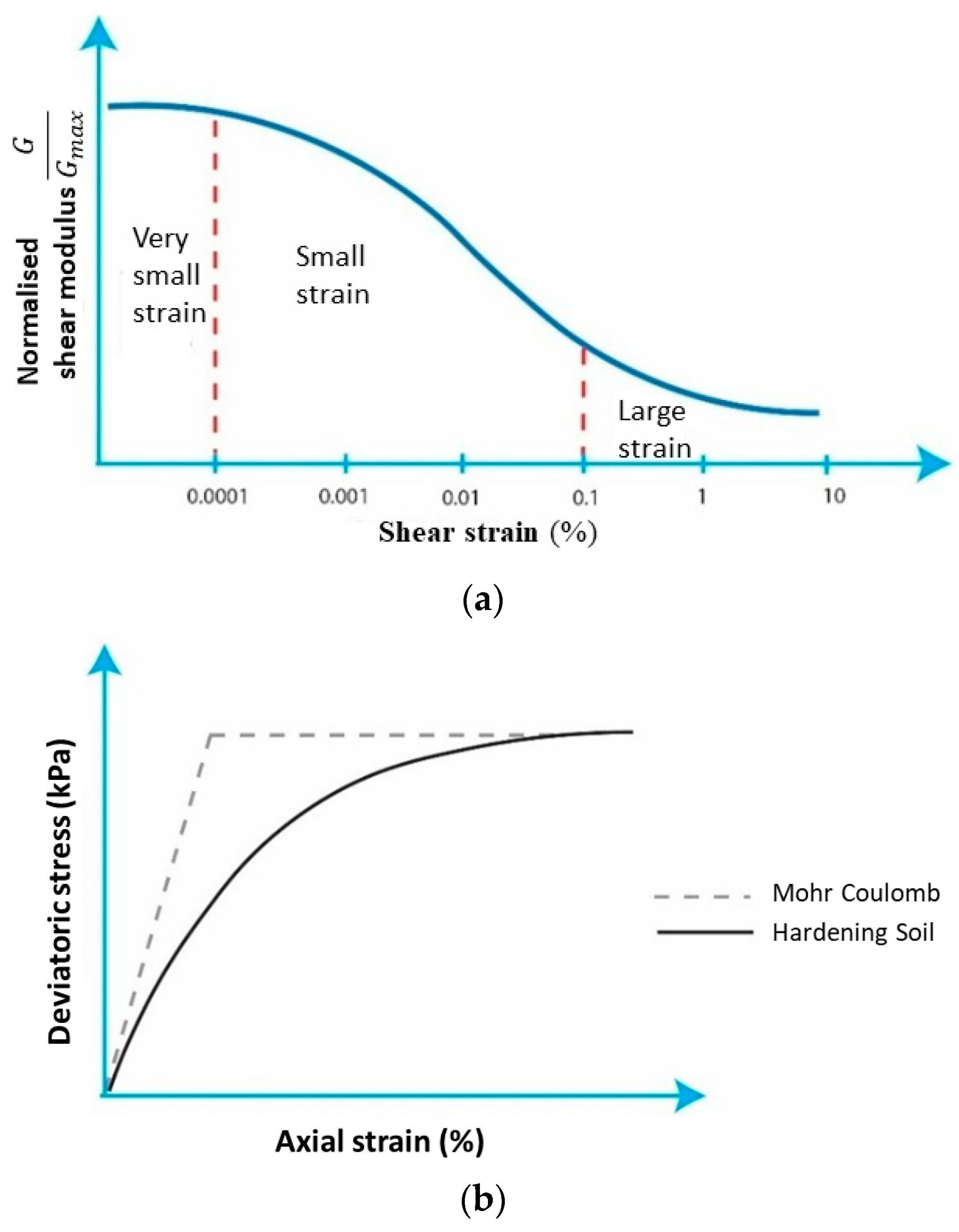
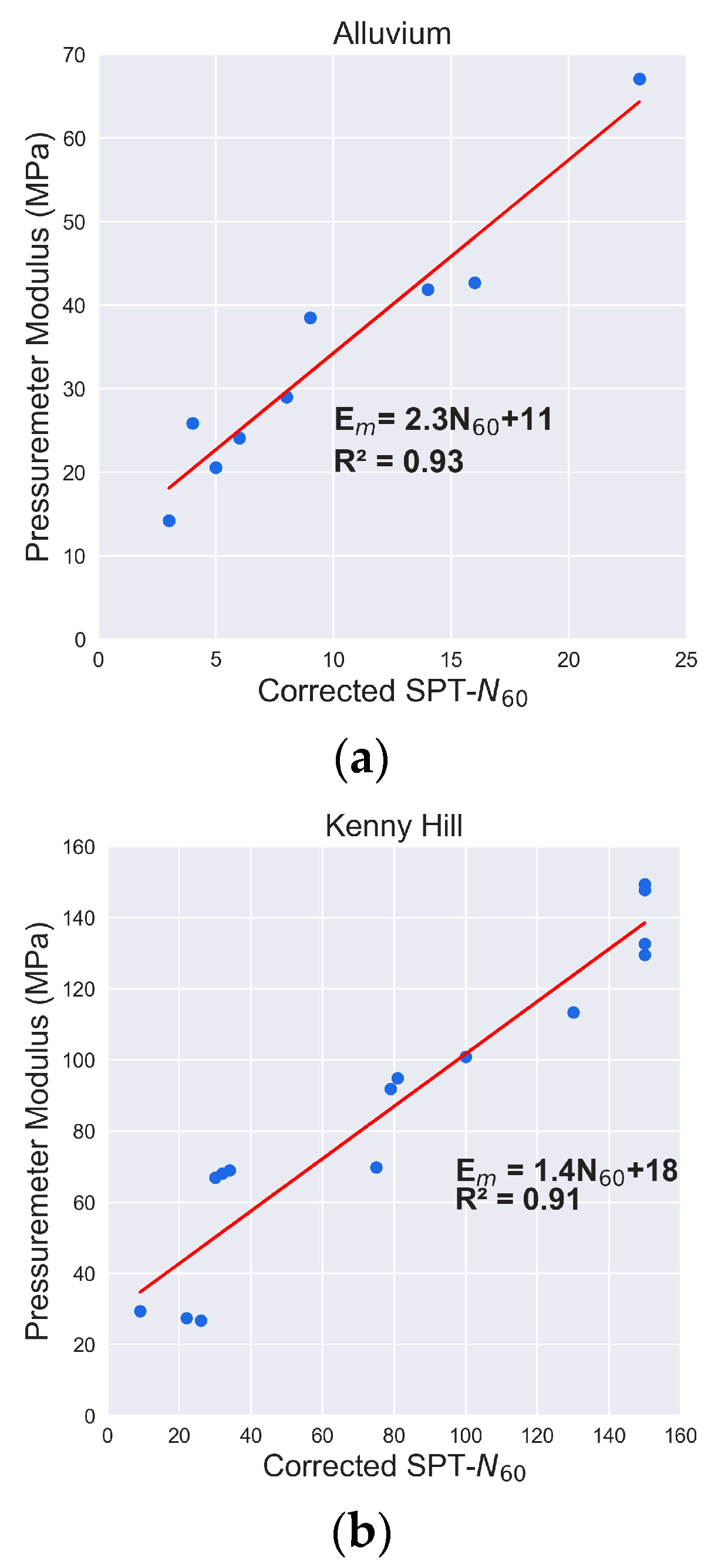
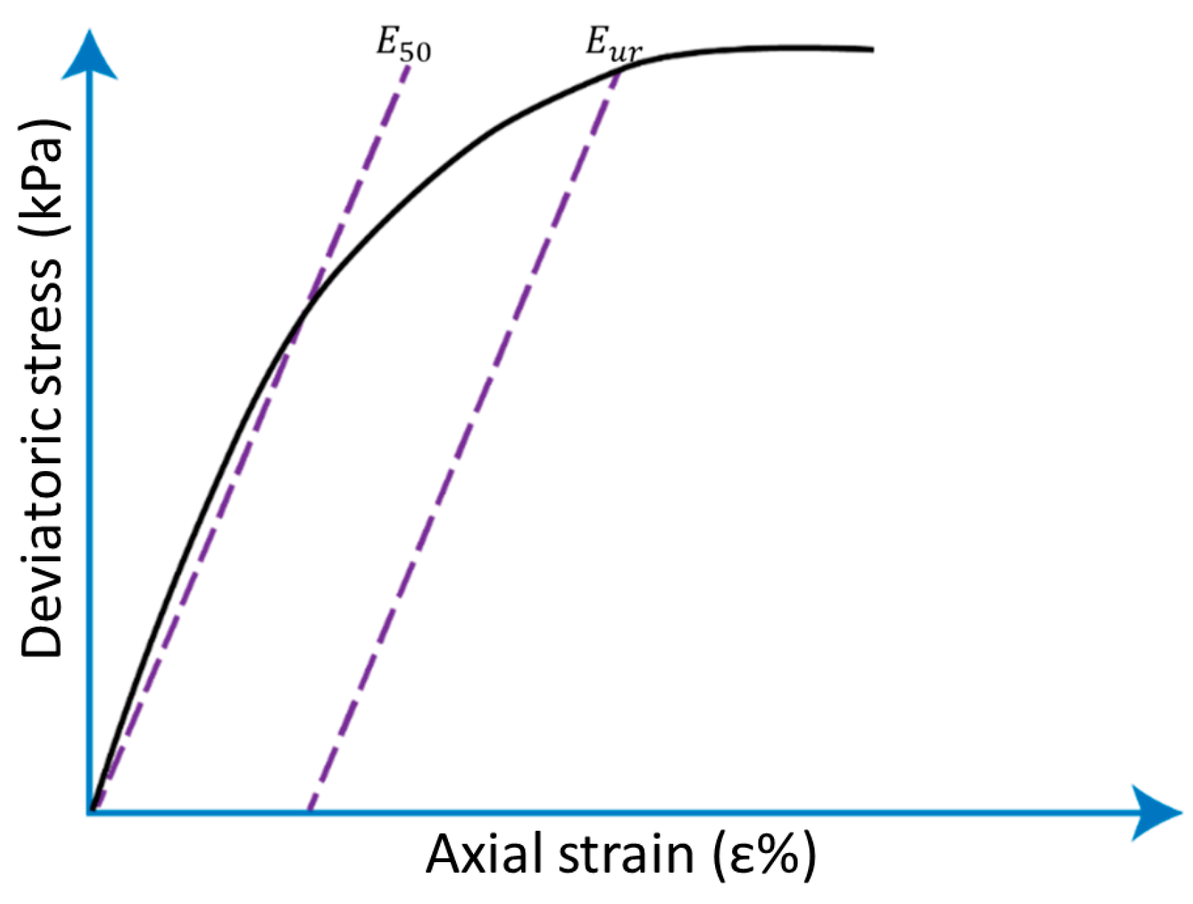
2.2. Interpretation of Geotechnical Parameters

To carry out the numerical analysis of any geotechnical application, the accuracy of the soil-structure interaction problems is crucial as the soil is the weakest material compared to others such as concrete and steel. Hence, the analysis is strongly dependent on the soil constitutive model to reflect the actual condition of the ground.
The soil profile for each model comprises two layers of soil and rock. The tunnels are bored through the soil layers (alluvium and Kenny Hill). Hence, the rock layer does not have an impact on the analysis. The range of soil stresses and strains are important in the analysis; hence, this shall be considered in the numerical analysis. For the finite element analysis, two common soil constitutive models were used by many researchers in relevant studies, which are Mohr-Coulomb (MC) [25,35] and Hardening Soil (HS) [36,37]. Gerhard [37] compared the MC and HS of the tunnelling finite element analysis and found that the MC model can provide higher settlement values in comparison with the measurements on the site, while the HS model predicts SS values that are closer to the actual measurements using the 2D grout pressure method. In addition, Hejazi et al. [38] found the SS induced by tunnelling is strongly influenced by the soil constitutive model. From their findings, MC SS appears unrealistic, which is due to the stiffness modulus in the MC model being constant at certain points of strain. Islam and Iskander [28] mentioned that MC is not able to stimulate the behaviour of the soil, especially during unloading and tunnel excavation. However, they stayed with the MC model due to the simplicity of the parameters. Moller [39] carried out both analyses using 2D and 3D finite element analysis for the second Heinenoord slurry shield using the HS model, and the findings showed the simulated SS is close to the site’s actual settlement values. His analysis results are aligned with another study conducted by Likitlersuang et al. [36], where they reported very close readings to the measured settlement using the HS model. Choon [40] emphasised that the soil constitutive models play a crucial role in the analysis results and concluded that tunnelling involves unloading and reloading the surrounding soils. Hence, the HS model was recommended by Choon [40] for use in the assessment of SS. In addition, Janin et al. [41] stated that the HS model can distinguish the stiffness modulus for the primary loading and unloading, which makes this numerical analysis closer to the measured SS results.
The soil properties can be classified by the strain levels into three categories, which are very small strain level (stiffness modulus is constant in elastic range), small strain level (stiffness modulus varies non-linearly with the strain), and large strain level (soil is close to the failure, and the soil stiffness is relatively small) where tunnelling works can be considered as large strain level [42]. The illustration of the categories of the strain level can be seen in Figure 4a. The HS model was created with the concept of plasticity, where the total strains of the soil are calculated using a stress-dependent stiffness that is different for both loading and unloading. The MC model indicates that the soil behaviour is linearly elastic and perfectly plastic. In addition, the HS model can consider loading and unloading stages, which can reflect the actual situation of tunnel construction for the removal of soil (unloading), followed by tunnel lining construction (loading). Therefore, the HS model is a more suitable soil model for the tunnel numerical analysis of tunnelling compared to MC [43]. An illustration of an indication of the difference between the MC and HS is shown in Figure 4b.
The soil parameter of effective strength is retrieved by carrying out consolidated isotopically undrained (CIU) tests from the closest boreholes at different depths. In addition, several Menard Pressuremetre Tests (PMTs) have been carried out as per BS 5930 [44] throughout the chainage of the tunnelling. The PMT was placed inside the borehole after the Standard Penetration Test (SPT-N) was taken. The depth of PMT was located at approximately the same depth as SPT-N, as this was conducted to ensure the data from SPT-N could be used as a reference for the comparison of similar lithologies. The corrected SPT-N was correlated with the pressuremetre modulus, Em. The previous researchers [45,46] carried out the correlation of the corrected SPT-N of N60 with the elastic modulus from the PMT. Some of the Em empirical formulas are presented in Table 3 according to different types of soil. The performance prediction of these formulas is presented based on the coefficient of determination (R2).
A total of 20 and 41 PMTs were carried out at the alluvium and Kenny Hill formations along the chainage of the tunnel, respectively. After carrying out the removal of outliers using the method of the interquartile range rule for a total of 61 PMTs, the corrected STP-N60 is plotted against Em for 2 different formations, as shown in Figure 5.
From the SPT-N, the selected section for the tunnelling analysis with a borehole is correlated with the elastic modulus according to the type of soil. However, E m is different from the soil elastic modulus; hence, conversion of the calculation is required. The difference could be due to several reasons, such as the difference in the range of radial, the stress surrounding the borehole wall, the possibility of disturbance during drilling and the installation of probes, and the computation of the modulus with the assumption of cylinder length as infinite [49]. Therefore, correction of the elastic modulus, E , of the soil is introduced to the actual value from E m [50], which is defined as follows:
α = E m E
where α is a Menard’s factor. In the HS model, there are three crucial elastic modulus inputs for the analysis, which are namely: secant stiffness modulus corresponding to 50% of the ultimate deviatoric stress, E 50 ; Oedometer modulus, E O e d ; and unloading or reloading modulus, E u r . Secant stiffness from the drained triaxial test at 50% of the ultimate deviatoric stress E 50 is the confining stress that depends on stiffness modulus for primary loading where the amount of stress is dependent on the power of m .
E 50 = E 50 r e f ( c cos Φ σ 3 sin Φ c cos Φ + P r e f sin Φ ) m
where pref is a reference stress of 100 kPa, c’ is effective cohesion, and Φ is effective friction angle. The stiffness is affected by minor effective principal stress. The power m governs the stress dependency. As reported by Janbu [51], the sand content of m is approximately 0.5. Other than this input, the reference oedometer modulus, E o e d R e f , acts as the parameter that controls the magnitude of the plastic strains that arise from the yield cap ε v p c . The oedometer modulus can be defined as follows:
E O e d = E O e d R e f ( c cos Φ σ 1 sin Φ c cos Φ + P r e f sin Φ ) m
where E o e d R e f is approximately similar to E 50 R e f [52] as illustrated in Figure 6. In addition, the stress-dependent stiffening modulus for unloading and reloading can be calculated as follows:
E u r = E u r R e f   ( c cos Φ σ 3 sin Φ c cos Φ + P r e f sin Φ ) m
For the ease of numerical computation, several researchers [40,53] have used E 50 R e f = 3 E u r R e f as per recommended by the previous researchers [52,54]. The input of E50 is correlated with the range from 0.06E to 0.26E with 0.5qf (where E is the elastic modulus of the soil and qf is the deviatoric stress from the secant stiffness modulus reduction curves from static torsional and triaxial shear data on clays and sands) [55]. Based on the interpretation, Table 4 summaries the geotechnical input parameters for these five models.
A total of 36 and 35 bulk density tests are carried out on the alluvium and Kenny Hill formations across the tunnelling alignment at various depths, respectively. The statistical input of bulk density is summarised in Table 5. In addition, the groundwater level recorded from the closest borehole with the readings recorded for morning and evening throughout the SI works will be used as part of the analysis, and these readings are taken as an average of the groundwater level. The groundwater level is one of the important parameters because when the groundwater level is lowered, it can cause a reduction in the pore pressure, which indirectly increases the surface settlement [56]. Figure 7 shows an illustration of how the lowering of groundwater causes the settlement.

2.3. Tunnel Boring Machine (TBM) Operational Parameters

Various operational factors of TBMs, including face pressures, rates of penetration, and pressures of grouting the tail void, jointly impact the surface settlement caused by mechanised tunnelling operations. TBMs cause surface settlement mainly by moving soil during excavation, resulting in empty spaces where the neighboring ground eventually subsides. While the TBM constructs the tunnel, it can also shift the ground, prompting settlement. The interplay between the tunnel lining and the nearby soil can trigger certain adaptations and shifts in the ground, indirectly resulting in surface settlement. Numerous studies [3,24] have demonstrated that face pressure and grouting pressure are the two important contributors to the SS caused by mechanised tunnelling. Hence, in this study, these two parameters were considered to be part of the finite element analysis. The EPB shield of the face pressure operates with the cutter head rotating, and cutting tools scrap the ground from the tunnel face while additives are injected into the material. The amount of the excavated soil is controlled and transported from the shield, and the tunnel face can be supported by the soil stored in the chamber. Hence, the face pressure stores in the chamber are crucial to maintaining the stability of the excavation. Different conditions of face pressure result in different SS scenarios. Several studies have found that increasing face pressure causes a decrease in settlement [3,57]. A different ideal scenario for the face pressure that affects the SS is illustrated in Figure 8. Case 1 shows that when the face pressures are equivalent to the overburden pressure, there are no impacts on the ground surface. Case 2 depicts the face pressures being less than the overburden pressures and the ground settling. Lastly, case 3 illustrates when the face pressures are more than the overburden pressures, heaving can be seen. Nevertheless, the amount of face pressure exceeded or lesser than the required pressures is subjected to the soil properties.
The shield diameter is larger than the external diameter of the installed lining, which causes a gap between the segments and the excavated soil mass [58]. This gap difference is known as a tail void or annulus, and it easily occupies the inward deforming soil during the shield and tail skin assembly process. When the tunnelling machine advances, the void can be continually filled with grout in one of two ways: by pumping the grout through pre-cast concrete lining segments or injecting the grout via grout ports at the back of the tail skin. The injection was carried out under high pressure in the tail void formed by the shield tail’s back. Thus, this is known as tail void grouting pressure. With high-pressure injection, the void can be filled within a short period of time with grouting material.
Other than these two parameters, another operating parameter that can be modelled into the numerical analysis is jack-force thrust. The distribution of the jack thrust in this study is uniform across the theoretical models. The function of this thrust force is to stimulate the actual condition of the mechanised tunnelling to move forward. The face pressure and grouting pressure, with the average input of the recorded face pressure and grouting pressure, are adopted in the analysis. To avoid the complication of the analysis, the value is rounded off to the nearest two significant values, and these numbers are summarised in Table 6.

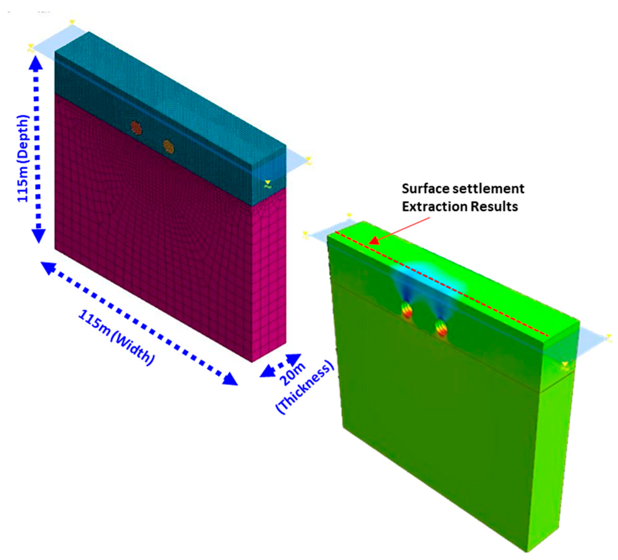
3. Construction of Numerical Model

3.1. General Characteristics

The numerical analysis was carried out using MIDAS GTX NX. In this section, the geometry dimension of the numerical model for the analysis will be further explained, the input for the grouting materials for the analysis will be stated, and the boundary condition of the model will be described.
Before the commencement modelling of the numerical analysis, the extended dimensions of the models affect the analysis required to be identified. In this analysis, the overall geometry of the numerical model was based on the recommendations by Alagha and Chapman [59] and Ruse [60]. Where C is the tunnel cover, D is the tunnel diameter, the recommendation for the minimum numerical model width is 2D, the depth of the model is C + 3D/2, and the length is 3D. Figure 9 shows a view of the models with various dimensions (x, y, and z directions). The overall adopted numerical model dimension is 115 m (width) × 115 m (depth) × 20 m (thickness). In this numerical model, the diameter of the tunnel is 6.7 m with a segmental lining width of 1.5 m. The tail void grout thickness is 150 mm. Two types of grouting were used in the analysis which are fresh and hardened grouting. The properties of the grouting materials are tabulated in Table 7. In addition, the degree of freedom for the numerical model was constrained in the x-direction, whereas in the y-direction was on both sides. Lastly, only nodes at the bottom were constrained in the z-direction. The top nodal along the ground surface was not constrained to allow the movement of the ground during the tunnelling process.

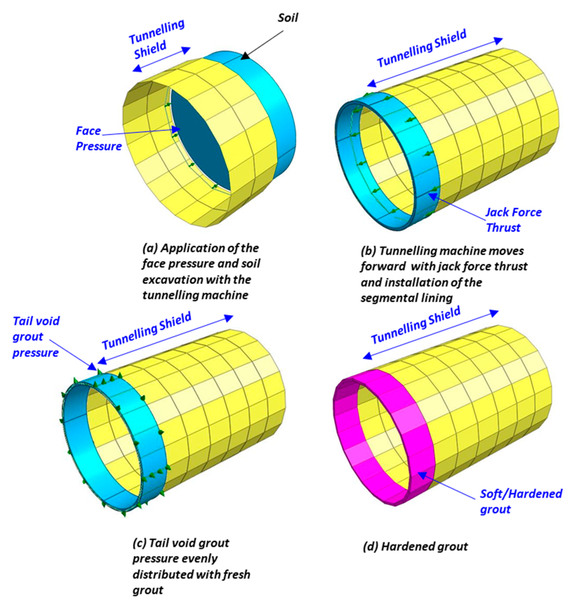
3.2. Construction Stages

Several stages have been involved in stimulating tunnel construction. In general, the process of tunnelling includes soil excavation, the installation of segment lining, and the application of external forces. At the beginning of the process, the self-weight and groundwater were activated to simulate the initial stage to establish the geostatic stresses in the soil mass. Subsequently, excavation was carried out by deactivating the soil elements with face pressure on the excavation face and, at the same time, activating the shield shell, which represents the tunnelling machine moving forward (Figure 10a). This process of excavation was repeated until the total length of the shield (equal to six segmental linings) was moved into the soil mass and the force thrust of tunnelling machine was activated to indicate the movement of tunnelling machine, and the segmental lining was installed at this stage (Figure 10b). Subsequently, the tail void grouting pressure was activated with fresh grout material (Figure 10c). Finally, the fresh grout was converted to hardened grout (Figure 10d) to show the later stage of the project. The tunnelling operational procedures of the numerical analysis for the tunnelling machine are shown in Figure 11. The different stages involved in tunnel construction, which encompasses excavation involving face pressure, lining installation, and grouting, exert an influence on SS. During excavation, voids are formed that cause the surrounding soil to settle. The installation of the lining can displace the ground, contributing to settlement as the tunnel’s supporting structure interacts with the soil. The grouting process, aimed at filling the gaps between the tunnel and the excavated area, affects the soil’s radial distribution, consequently impacting SS. Each of these phases brings about distinct settlement effects, and the overall sequence and coordination of these stages play a pivotal role in effectively managing settlement levels.

4. Results and Discussion

In this section, the output SS from the numerical analysis is compared with field measurements of SS, and the interpretation of the results will be further discussed. A total of five numerical models were analysed and compared with the measured settlement at the site. A total of five models’ geometries can be found in Table 8. One of the tunnel geometries that impacts the SS between twin tunnels is the pillar width. Based on Table 8, it can be observed that Model 1, with the shortest pillar width, exhibits the highest SS between the tunnels. This implies that both the 1st and 2nd bored tunnels contribute to the maximum SS occurring between them.
The field measurements of SS directly above each bored tunnel closely align with the results obtained from the numerical analysis, as presented in Table 9. A comparison between the numerical analysis and the actual measurements is conducted in terms of percentage differences. The disparities are predominantly below 18% across most models, with the exception of Model 2 of the second bored tunnel, where a notably higher percentage difference of 28.6% is observed. In comparison with the actual measurement, only a minor difference of 1 mm is observed between the actual value and the analysis. In general, the difference between measured and actual measurement is in the range of 0.5 mm to 3.1 mm.
Additionally, the SS values obtained from measurements and numerical analysis for both the first and second bored tunnels are graphically represented in Figure 11, with coefficient of determination (R2) values of 0.94 and 0.96 for the first and second bored tunnel SS, respectively. These high R2 values suggest strong correlations between the measured and computed SS values for both tunnels.
The SS output of the numerical analysis for each model is visualised alongside the corresponding field measurement, as depicted in Figure 12. Observing the patterns within Figure 12, it can be seen that the 3D numerical analysis of the tunnel construction process effectively approximates the measured SS.
The output of this analysis has shown close similarities between the prediction settlement using MIDAS software and the site measurement. Model 1 has the shortest pillar width (6 m) in comparison with all the models. From this model, it can be seen that the 1st and 2nd bored tunnels do not have much difference (2 mm); however, the maximum SS is found located in between these two tunnels with the shape of a single symmetric settlement trough, which is similar to the findings as per Peck [5] and Likitlersuang et al. [36].
Model 2 depicts the unique trend of SS, where the maximum SS is found at the 1st bored tunnel instead of the 2nd bored tunnel. In the actual scenario of excavation for twin tunnels, the first bored tunnel excavates the undisturbed soil. However, the process of excavation for the first bored tunnel disturbed the soil surrounding it. Hence, this will cause the second tunnel’s soil to be disturbed. Terzaghi [61] was the first researcher who published a paper related to the field data of surface settlements above twin tunnels. His findings showed that the settlements above the second tunnel are larger than the first tunnel. However, based on the result of the analysis and the site-recorded SS, the second bore tunnel does not have the highest SS. In the past, most of the tunnelling operations for twin tunnels were carried out using compressed air [62]. In addition, several researchers [63,64] have found that the settlements above the second tunnels were larger than the first tunnels. The finding that the second bored tunnel has the maximum SS is applicable for open-face tunnelling because the ground reaction is influenced by tunnel geometry and geological conditions.
It is obvious that the SS values above the second tunnel could be lower. This is because the tunnelling operational parameters are considered contributing factors to the settlement [65]. Kannangara et al. [66] also found a similar trend in the outputs, where the observed second excavated tunnel has a lower SS when the face and grouting pressure are controlled at the same or higher margin compared with the first excavation. Although Model 3 has an approximately similar pillar width to Model 2 (different by 1 m) with a deeper depth, the 1st and 2nd bored tunnel SS do not have many differences. This could be due to the similarities in the operation parameters between the two tunnels and the deeper tunnel depth. Hence, these two bored tunnel SS of Model 3 have more consistent SS compared to Model 2.
Model 5 exhibits the highest settlement in comparison to the remaining models due to the lowest soil stiffness of the ground. It can be inferred that when twin tunnels have a larger spacing of 3D, there is no interaction between the tunnels [28]. This is evident from Model 4, where the maximum surface settlement at the 1st excavated tunnel is likely due to slightly low face pressure. Consequently, it can be deduced that within this range of pillar width, there is no impact from the first bored tunnel on the area of the second tunnel.
Several researchers have also carried out the analysis of tunnelling using MIDAS software and reported very close findings to the measured settlement for the different scenarios of the analysis as tabulated in Table 10.
In previous studies, the most common method to determine the surface settlement induced by tunnelling is the empirical formula. This empirical formula is dependent on the VL, which varies according to the type of ground and installation tunnel. However, as far as the authors know, no literature on VL for the soil in Malaysia has been published. The use of empirical formulas is limited to certain ground conditions and installation methods. Chakeri and Ünver [69] compared the empirical formula with the measured settlement, and from their studies, the calculated and measured settlement diverge by more than two times. In addition, they also carried out the 3D numerical analysis; however, the 3D numerical analysis was carried out in the lithology of the ground for the Gungoren formation, which mainly consists of very stiff clay, hard clay, and dense sand. Furthermore, Choon [40] used the 2D finite element of the contraction method with various VL inputs to retrieve a similar SS as measured at the site. Furthermore, several studies [70,71,72] have utilised centrifuge laboratory modelling for sandy soil materials. However, these laboratory results have not been compared with field measurements, and they have not taken tunnelling operational parameters into consideration. Therefore, by utilising 3D numerical analysis, it becomes possible to integrate three crucial factors: tunnel geometry, geotechnical soil properties, and tunnelling operational parameters. This integration, combined with the incorporation of tunnelling machine construction processes, allows for the accurate determination of SS. This approach mitigates the constraints associated with alternative methodologies, as discussed previously. Consequently, this demonstrates that this method offers superior advantages compared to other approaches.

5. Limitations and Future Works

In this study, the number of field measurements is limited due to the focused investigation on the alluvium and Kenny Hill formation areas. Therefore, expanding the scope to include more field measurements from various locations, particularly within the soil area, with closer intervals would enhance the development and validation of the model. Additionally, if the budget allows, considering real-time monitoring for tunnelling-induced settlement measurements could be beneficial.
It is important to note that the geological profile is established based on the closest SI boreholes with a diameter of 100 mm, which implies a potential non-homogeneity in the studied geological profile. Furthermore, the input of groundwater levels relies on recorded SI works, which could be influenced by field conditions.
While 3D numerical modelling is time-consuming and unsuitable for real-time analysis during the operation of long tunnels, situations involving geological formations and tunnel operational parameters may arise. Therefore, new computational approaches such as machine learning and intelligent techniques could find applications in this context. Combining these approaches with established theories and empirical equations in relevant domains could yield a more generalised technique for predicting settlement induced by twin tunnels. Moreover, these techniques would offer practicality and relevance to engineers in the field.

6. Conclusions

The findings from the 3D numerical analysis of parallel tunnels using the MIDAS software, incorporating mechanised tunnelling construction stages and a hardening soil model, demonstrate an acceptable level of prediction accuracy for SS when compared with field measurements. Consequently, the industry may consider adopting this approach for SS assessment. Furthermore, the 3D numerical modelling approach enables the customization of mitigation strategies for SS based on specific project parameters, aiming to achieve a more sustainable tunnel construction. The key findings of this investigation can be summarised as follows:
(1)
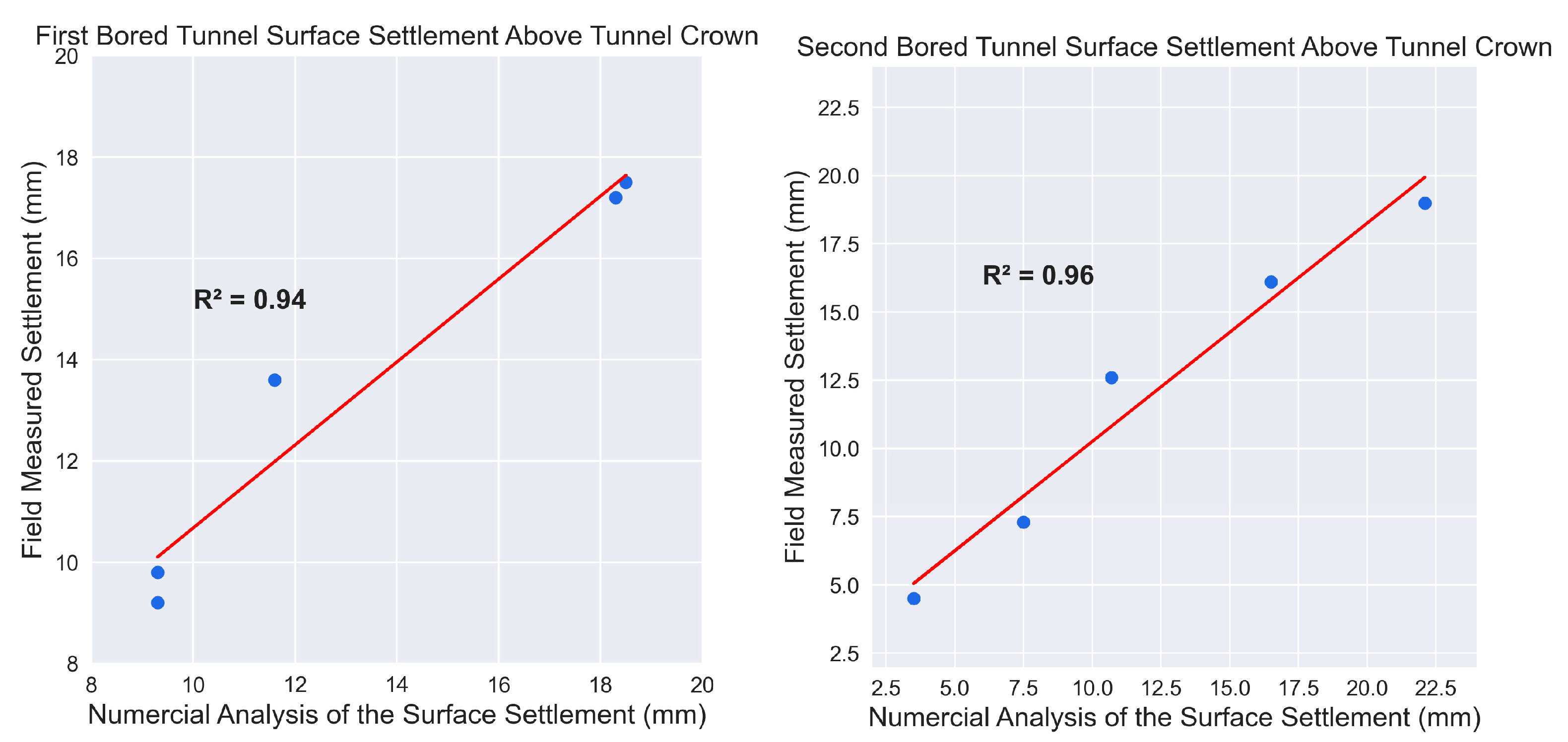
The 3D numerical analysis produced SS above the tunnel crown of twin tunnels has shown R2 = 0.94 and R2 = 0.96, respectively for the first and second bored tunnels with the actual field measurements and the largest difference settlement of 3.1 mm.
(2)
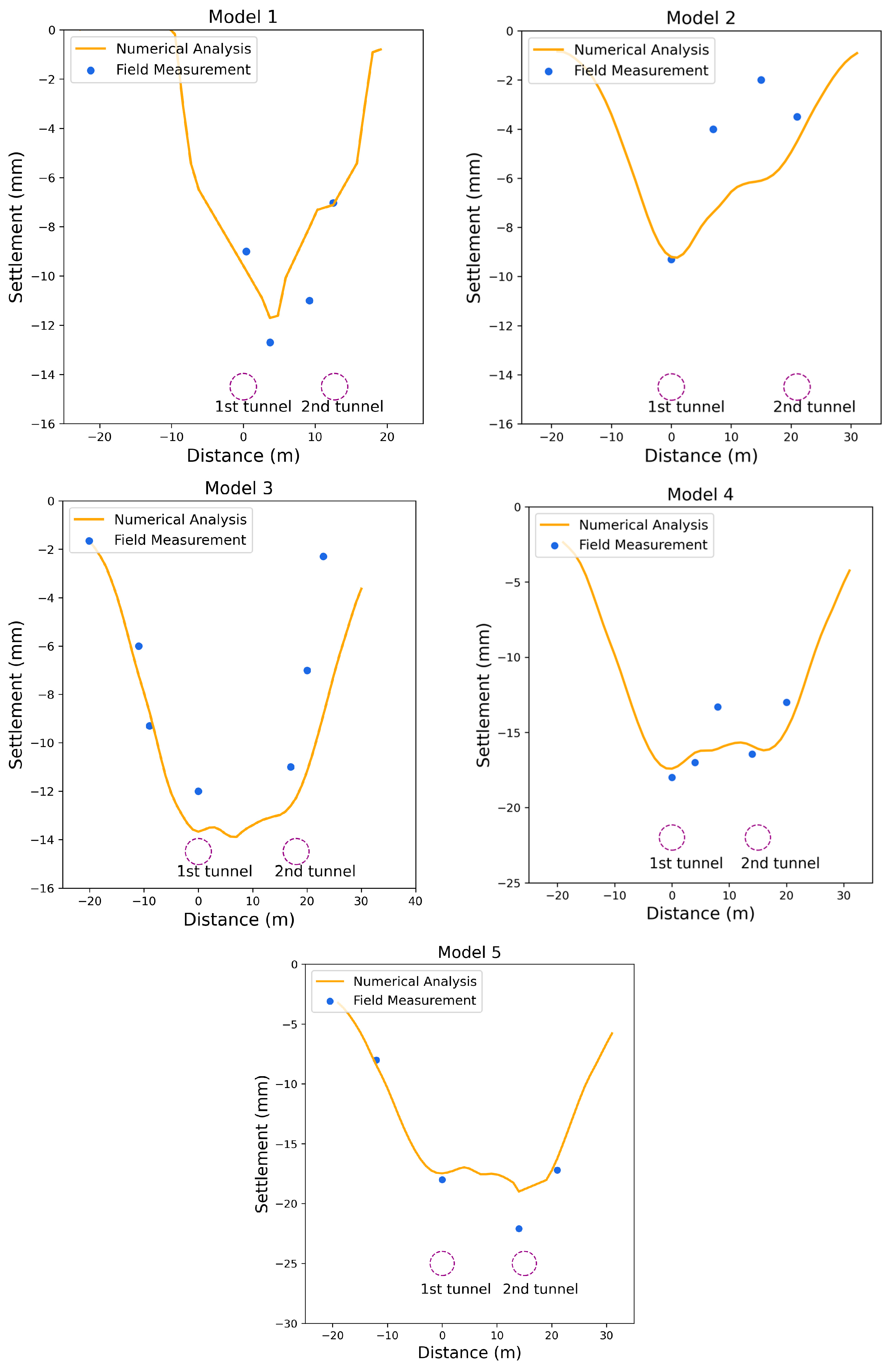
The second bored tunnel does not consistently exhibit the largest SS because it can be influenced by other factors, such as tunnel geometry, geotechnical soil properties, and tunnel operational parameters. For example, a narrower pillar width can lead to higher SS between tunnels, as demonstrated in Model 1. Similarly, areas with lower soil stiffness could also result in elevated SS. Additionally, insufficient face pressure can contribute to increased settlement.
(3)
It can be stated that no effect of the first bored tunnel on the second bored tunnel area at a distance of equal or more than 3D between the tunnels has been observed.
(4)
The interpretation of the elastic modulus from the field pressuremetre test and SPT-N can be used as geotechnical soil stiffness parameter inputs in the numerical analysis. The interpreted relationship of the pressuremetre modulus with corrected SPT-N is as follows: E m = 2.3   N 60 + 11 (alluvium) and E m = 1.4   N 60 + 18 (kenny Hill).
(5)
Three main input parameters, namely tunnel geometry, engineering ground parameters, and tunnel operational parameters, considered in the numerical analysis yield results that closely align with the field measurements.

Author Contributions

Conceptualization, C.Y.H., S.H.L., D.J.A., H.R. and X.H.; methodology, C.Y.H., S.H.L. and D.J.A.; software, C.Y.H., S.H.L. and D.J.A.; validation, C.Y.H., S.H.L. and D.J.A.; formal analysis, C.Y.H., S.H.L. and D.J.A.; resources, C.Y.H. and S.H.L.; data curation, C.Y.H. and D.J.A.; writing—original draft preparation, C.Y.H., S.H.L., D.J.A., H.R. and X.H.; writing—review and editing, C.Y.H., S.H.L., D.J.A., H.R. and X.H.; supervision, S.H.L., D.J.A., H.R. and X.H. All authors have read and agreed to the published version of the manuscript.

Funding

This research received no external funding.

Institutional Review Board Statement

Not applicable.

Informed Consent Statement

Not applicable.

Data Availability Statement

The data will be available upon a reasonable request.

Acknowledgments

The authors would like to extend their sincere gratitude to Mass Rapid Transit Corporation Sdn Bhd, the contractor (MMC Gamuda KVMRT Sdn Bhd) and the consultant (G&P Geotechnics Sdn Bhd) for facilitating this study. The authors would also like to express appreciation to Universiti Malaya for supporting this research.

Conflicts of Interest

The authors declare no conflict of interest.

References

  1. Chen, R.; Li, J.; Kong, L.; Tang, L. Experimental study on face instability of shield tunnel in sand. Tunn. Undergr. Sp. Technol. 2013, 33, 12–21. [Google Scholar] [CrossRef]
  2. Wan, C.; Jin, Z. Adaptability of the cutter-head of the earth pressure balance (epb) shield machine in water-rich sandy and cobble strata: A case study. Adv. Civ. Eng. 2020, 2020, 8847982. [Google Scholar] [CrossRef]
  3. Ahmed, N.Z.; El-Shourbagy, M.; Akl, A.; Metwally, K. Field monitoring and numerical analysis of ground deformation induced by tunnelling beneath an existing tunnel. Cogent Eng. 2021, 8, 1861731. [Google Scholar] [CrossRef]
  4. Hasanipanah, M.; Noorian-Bidgoli, M.; Armaghani, D.J.; Khamesi, H. Feasibility of PSO-ANN model for predicting surface settlement caused by tunnelling. Eng. Comput. 2016, 32, 705–715. [Google Scholar] [CrossRef]
  5. Peck, R.B. Deep Excavations and Tunneling in Soft Ground. In Proceedings of the 7th International Conference on Soil Mechanics and Foundation Engineering, Mexico City, Mexico, 1969; pp. 225–290. Available online: http://scholar.google.com/scholar?hl=en&btnG=Search&q=intitle:Deep+excavations+and+tunneling+in+soft+ground#0%5Cnhttp://ci.nii.ac.jp/naid/10007809489/ (accessed on 30 August 2023).
  6. Litwiniszyn, J. Application of the equation of stochastic processes to mechanics of loose bodies. Arch. Mech. Stos. 1956, 8, 393–411. [Google Scholar]
  7. Clough, G.W.; Leca, E. EPB shield tunneling in mixed face conditions. J. Geotech. Eng. 1993, 119, 1640–1656. [Google Scholar] [CrossRef]
  8. Suwansawat, S.; Einstein, H.H. Artificial neural networks for predicting the maximum surface settlement caused by EPB shield tunnelling. Tunn. Undergr. Sp. Technol. 2006, 21, 133–150. [Google Scholar] [CrossRef]
  9. Attewell, P.B.; Farmer, I.W. Ground disturbance caused by shield tunnelling in a stiff, overconsolidated clay. Eng. Geol. 1974, 8, 361–381. [Google Scholar] [CrossRef]
  10. O’Reilly, M.P.; New, B.M. Settlements above Tunnels in the United Kingdom—Their Magnitude and Prediction; Institution of Mining & Metallurgy: Carlton, Australia, 1982. [Google Scholar]
  11. Mair, R.J.; Taylor, R.N. Bored tunnelling in the urban environments. In Proceedings of the Fourteenth International Conference on Soil Mechanics and Foundation Engineering, Hamburg, Germany, 6–12 September 1997. [Google Scholar]
  12. Wan, M.S.P.; Standing, J.R.; Potts, D.M.; Burland, J.B. Measured short-term ground surface response to EPBM tunnelling in London Clay. Geotechnique 2017, 67, 420–445. [Google Scholar] [CrossRef]
  13. Rezaei, A.H.; Ahmadi-adli, M. The volume loss: Real estimation and its effect on surface settlements due to excavation of Tabriz Metro tunnel. Geotech. Geol. Eng. 2020, 38, 2663–2684. [Google Scholar] [CrossRef]
  14. Le, B.T.; Nguyen, T.T.T.; Divall, S.; Davies, M.C.R. A study on large volume losses induced by EBPM tunnelling in sandy soils. Tunn. Undergr. Sp. Technol. 2023, 132, 104847. [Google Scholar] [CrossRef]
  15. Mair, R.J.; Taylor, R.N.; Bracegirdle, A. Subsurface settlement profiles above tunnels in clays. Geotechnique 1993, 43, 315–320. [Google Scholar] [CrossRef]
  16. Loganathan, N.; Poulos, H.G. Analytical prediction for tunneling-induced ground movements in clays. J. Geotech. Geoenvironmental Eng. 1998, 124, 846–856. [Google Scholar] [CrossRef]
  17. Wang, H.; Sun, H.; Jin, H. The influence and calculation method of ground settlement induced by tunnel construction in sand. J. Chin. Inst. Eng. 2020, 43, 681–693. [Google Scholar] [CrossRef]
  18. Zhu, B.; Zhang, P.; Lei, M.; Wang, L.; Gong, L.; Gong, C.; Chen, F. Improved analytical solution for ground movements induced by circular tunnel excavation based on ground loss correction. Tunn. Undergr. Sp. Technol. 2023, 131, 104811. [Google Scholar] [CrossRef]
  19. Lee, K.M.; Rowe, R.K.; Lo, K.Y. Subsidence owing to tunnelling. I. Estimating the gap parameter. Can. Geotech. J. 1992, 29, 929–940. [Google Scholar] [CrossRef]
  20. Vermeer, P.A.; Brinkgreve, R. Plaxis Version 5 Manual; Balkema, A.A., Ed.; PLAXIS MoDeTo: Rotterdam, The Netherlands, 1993. [Google Scholar]
  21. Addenbrooke, T.I.; Potts, D.M.; Puzrin, A.M. The influence of pre-failure soil stiffness on the numerical analysis of tunnel construction. Géotechnique 1997, 47, 693–712. [Google Scholar] [CrossRef]
  22. Surarak, C. Geotechnical Aspects of the Bangkok MRT Blue Line Project; Griffith University: Nathan, Australia, 2011. [Google Scholar]
  23. Mair, R.J. Centrifugal Modelling of Tunnel Construction in Soft Clay. Ph.D. Thesis, University of Cambridge, Cambridge, UK, 1980. [Google Scholar]
  24. Wongsaroj, J.; Borghi, F.X.; Soga, K.; Mair, R.J.; Sugiyama, T.; Hagiwara, T.; Bowers, K.H. Effect of TBM driving parameters on ground surface movements: Channel Tunnel Rail Link Contract 220. Geotech. Asp. Undergr. Constr. Soft Gr. 2005, 335–341. [Google Scholar]
  25. Lai, J.; Zhou, H.; Wang, K.; Qiu, J.; Wang, L.; Wang, J.; Feng, Z. Shield-driven induced ground surface and Ming Dynasty city wall settlement of Xi’an metro. Tunn. Undergr. Sp. Technol. 2020, 97, 103220. [Google Scholar] [CrossRef]
  26. Mathew, G.V.; Lehane, B.M. Numerical back-analyses of greenfield settlement during tunnel boring. Can. Geotech. J. 2013, 50, 145–152. [Google Scholar] [CrossRef]
  27. Lu, D.; Li, X.; Du, X.; Lin, Q.; Gong, Q. Numerical simulation and analysis on the mechanical responses of the urban existing subway tunnel during the rising groundwater. Tunn. Undergr. Sp. Technol. 2020, 98, 103297. [Google Scholar] [CrossRef]
  28. Islam, M.S.; Iskander, M. Effect of Geometric Parameters and Construction Sequence on Ground Settlement of Offset Arrangement Twin Tunnels. Geosciences 2022, 12, 41. [Google Scholar] [CrossRef]
  29. Cuvier, G.; Knight, D. Essay on the Theory of the Earth; Routledge: Oxfordshire, UK, 2018. [Google Scholar]
  30. Taylor, R. A key to the Knowledge of Nature; or an Exposition of the Mechanical; Chemical, and Physical Laws Imposed on Matter by the Wisdom of the Almighty; Baldwin, Cradock, and Joy: London, UK, 1825. [Google Scholar]
  31. Woodward, J. The Ice Age: A Very Short Introduction; Oxford University Press: Oxford, UK, 2014. [Google Scholar]
  32. Lee, C.P. Scarcity of fossils in the Kenny Hill formation and its implications. Gondwana Res. 2001, 4, 675–677. [Google Scholar] [CrossRef]
  33. Law, K.H.; Othman, S.Z.; Hashim, R.; Ismail, Z. Determination of soil stiffness parameters at a deep excavation construction site in Kenny Hill Formation. Measurement 2014, 47, 645–650. [Google Scholar] [CrossRef]
  34. Malaysia, G.S. Bedrock Geology of Kuala Lumpur, Scale 1:25,000, Wilayah Persekutuan L8010 Part of Sheet 94k; Jabatan Mineral dan Geosains: Kuala Lumpur, Malaysia, 1993. [Google Scholar]
  35. Xie, X.; Yang, Y.; Ji, M. Analysis of ground surface settlement induced by the construction of a large-diameter shield-driven tunnel in Shanghai. China. Tunn. Undergr. Sp. Technol. 2016, 51, 120–132. [Google Scholar] [CrossRef]
  36. Likitlersuang, S.; Surarak, C.; Suwansawat, S.; Wanatowski, D.; Oh, E.; Balasubramaniam, A. Simplified finite-element modelling for tunnelling-induced settlements. Geotech. Res. 2014, 1, 133–152. [Google Scholar] [CrossRef]
  37. Gerhard, V.v.S. Numerical Analysis of Surface Settlements Induced by a Fluid-Supported Tunnelling Machine. 2012. Available online: https://diglib.tugraz.at/download.php?id=576a77b147200&location=browse (accessed on 30 August 2023).
  38. Hejazi, Y.; Dias, D.; Kastner, R. Impact of constitutive models on the numerical analysis of underground constructions. Acta Geotech. 2008, 3, 251–258. [Google Scholar] [CrossRef]
  39. Moller, S. Tunnel Induced Settlements and Structural Forces in Linings. 2006. Available online: http://www.uni-s.de/igs/content/publications/Docotral_Thesis_Sven_Moeller.pdf (accessed on 30 August 2023).
  40. Choon, C.H. Field Measurements and Numerical Analysis of Interaction between Closely Spaced Bored Tunnels. Ph.D. Thesis, Nanyang Technological University, Singapore, 2016. [Google Scholar]
  41. Janin, J.P.; Dias, D.; Emeriault, F.; Kastner, R.; Le Bissonnais, H.; Guilloux, A. Numerical back-analysis of the southern Toulon tunnel measurements: A comparison of 3D and 2D approaches. Eng. Geol. 2015, 195, 42–52. [Google Scholar] [CrossRef]
  42. Atkinson, J.H.; Sallfors, G. Experimental determination of soil properties. General Report to Session 1. In Proceedings of the 10th European Conference on Soil Mechanics and Foundation Engineering, Florence, Italy, 26–30 May 1991; pp. 915–956. [Google Scholar]
  43. Vitali, O.P.M.; Celestino, T.B.; Bobet, A. Construction strategies for a NATM tunnel in São Paulo, Brazil, in residual soil. Undergr. Sp. 2022, 7, 1–18. [Google Scholar] [CrossRef]
  44. BS 5930; Code of Practice for Site Investigations. Br. Stand. Inst. (BSI): London, UK, 1981.
  45. Ohya, S.; Imai, T.; Matsubara, M. Relationships between N value by SPT and LLT pressuremeter results. In Proceedings of the 2nd European Symposium on Penetration Testing, Amsterdam, The Netherlands, 24–27 May 1982; pp. 125–130. [Google Scholar]
  46. Yagiz, S.; Akyol, E.; Sen, G. Relationship between the standard penetration test and the pressuremeter test on sandy silty clays: A case study from Denizli. Bull. Eng. Geol. Environ. 2008, 67, 405–410. [Google Scholar] [CrossRef]
  47. Cheshomi, A.; Ghodrati, M. Estimating Menard pressuremeter modulus and limit pressure from SPT in silty sand and silty clay soils. A case study in Mashhad, Iran. Geomech. Geoengin. 2015, 10, 194–202. [Google Scholar] [CrossRef]
  48. Naseem, A.; Jamil, S.M. Development of correlation between standard penetration test and pressuremeter test for clayey sand and sandy soil. Soil Mech. Found. Eng. 2016, 53, 98–103. [Google Scholar] [CrossRef]
  49. Briaud, J.L. The Pressuremeter; AA Balkema: Rotterdam, The Netherlands, 1992. [Google Scholar]
  50. Gambim, M.; Rosseau, J. Interpretation and application of pressuremeter test results to foundation design. Gen. Memo. Rev. Sols Soils 1975, 26. [Google Scholar]
  51. Janbu, N. Soil compressibility as determined by oedometer and triaxial tests Wiesbaden. In Proceedings of the European Conference SMFE, Wiesbaden, Germany, 1963. [Google Scholar]
  52. Schanz, T.; Vermeer, P.A. On the stiffness of sands. In Pre-Failure Deform. Behav. Geomaterials; Thomas Telford Publishing: London, UK, 1998; pp. 383–387. [Google Scholar]
  53. Surarak, C.; Likitlersuang, S.; Wanatowski, D.; Balasubramaniam, A.; Oh, E.; Guan, H. Stiffness and strength parameters for hardening soil model of soft and stiff Bangkok clays. Soils Found. 2012, 52, 682–697. [Google Scholar] [CrossRef]
  54. Schanz, T.; Vermeer, P.A.; Bonnier, P.G. The hardening soil model: Formulation and verification. In Beyond 2000 Comput. Geotech.; Routledge: Oxfordshire, UK, 2019; pp. 281–296. [Google Scholar]
  55. Mayne, P.W. Integrated ground behavior: In-situ and lab tests. Deform. Charact. Geomater. 2005, 2, 155–177. [Google Scholar]
  56. Yoo, C.; Lee, Y.; Kim, S.-H.; Kim, H.-T. Tunnelling-induced ground settlements in a groundwater drawdown environment—A case history. Tunn. Undergr. Sp. Technol. 2012, 29, 69–77. [Google Scholar] [CrossRef]
  57. Shirlaw, J.N.; Ong, J.C.W.; Rosser, H.B.; Tan, C.G.; Osborne, N.H.; Heslop, P.E. Local settlements and sinkholes due to EPB tunnelling. Proc. Inst. Civ. Eng. Eng. 2003, 156, 193–211. [Google Scholar] [CrossRef]
  58. Greenwood, J. 3D Analysis of Surface Settlement in Soft Ground Tunnelling. 2002. Available online: http://hdl.handle.net/1721.1/29558 (accessed on 30 August 2023).
  59. Alagha, A.S.N.; Chapman, D.N. Numerical modelling of tunnel face stability in homogeneous and layered soft ground. Tunn. Undergr. Sp. Technol. 2019, 94, 103096. [Google Scholar] [CrossRef]
  60. Ruse, N.M. Räumliche Betrachtung der Standsicherheit der Ortsbrust beim Tunnelvortrieb; Institut für Geotechnik: Hanover, Germany, 2004. [Google Scholar]
  61. Terzaghi, K. Shield Tunnels of the Chicago Subway; Harvard University, Graduate School of Engineering: Cambridge, MA, USA, 1942. [Google Scholar]
  62. Islam, M.S.; Iskander, M. Twin tunnelling induced ground settlements: A review. Tunn. Undergr. Sp. Technol. 2021, 110, 103614. [Google Scholar] [CrossRef]
  63. Bartlett, J.V.; Bubbers, B.L. Surface movements caused by bored tunnelling. In Proceedings of the Conference on Subway Construction, Budapest, Hungary, 1970; pp. 513–539. [Google Scholar]
  64. Moretto, O. Discussion on “Deep excavations and tunnelling in soft ground”. In Proceedings of the 7th International Conference on Soil Mechanics and Foundation Engineering, Mexico City, Mexico, 1969; pp. 311–315. [Google Scholar]
  65. Suwansawat, S.; Einstein, H.H. Describing settlement troughs over twin tunnels using a superposition technique. J. Geotech. Geoenviron. Eng. 2007, 133, 445–468. [Google Scholar] [CrossRef]
  66. Kannangara, K.K.P.M.; Ding, Z.; Zhou, W.-H. Surface settlements induced by twin tunneling in silty sand. Undergr. Sp. 2022, 7, 58–75. [Google Scholar] [CrossRef]
  67. Zhou, Z.; Ding, H.; Miao, L.; Gong, C. Predictive model for the surface settlement caused by the excavation of twin tunnels. Tunn. Undergr. Sp. Technol. 2021, 114, 104014. [Google Scholar] [CrossRef]
  68. Ayasrah, M.; Qiu, H.; Zhang, X. Influence of cairo metro tunnel excavation on pile deep foundation of the adjacent underground structures: Numerical study. Symmetry 2021, 13, 426. [Google Scholar] [CrossRef]
  69. Chakeri, H.; Ünver, B. A new equation for estimating the maximum surface settlement above tunnels excavated in soft ground. Environ. Earth Sci. 2014, 71, 3195–3210. [Google Scholar] [CrossRef]
  70. Lu, H.; Shi, J.; Wang, Y.; Wang, R. Centrifuge modeling of tunneling-induced ground surface settlement in sand. Undergr. Sp. 2019, 4, 302–309. [Google Scholar] [CrossRef]
  71. Moussaei, N.; Khosravi, M.H.; Hossaini, M.F. Physical modeling of tunnel induced displacement in sandy grounds. Tunn. Undergr. Sp. Technol. 2019, 90, 19–27. [Google Scholar] [CrossRef]
  72. Athar, M.F.; Sadique, M.R.; Alsabhan, A.H.; Alam, S. Ground Settlement Due to Tunneling in Cohesionless Soil. Appl. Sci. 2022, 12, 3672. [Google Scholar] [CrossRef]
Figure 2. Example of installed ground settlement marker.
Sustainability 15 13265 g002
Figure 3. Illustration of the ideal position of settlement marker arrays along the twin tunnels.
Sustainability 15 13265 g003
Figure 4. (a) Normalised stiffness degradation curve [42], and (b) Triaxial drained compression stress of MC and HS models [43].
Sustainability 15 13265 g004
Figure 5. SPT-N (N60 against E m ) for (a) Alluvium, (b) and Kenny Hill.
Sustainability 15 13265 g005
Figure 6. Hyperbolic stress-strain relationship for the E 50 and E u r [52].
Sustainability 15 13265 g006
Figure 7. Lowered groundwater causes surface settlement [56].
Sustainability 15 13265 g007
Figure 8. Illustration of the face pressure on the surface settlement in different cases.
Sustainability 15 13265 g008
Figure 9. A numerical model for simulating SS induced by twin tunnels.
Sustainability 15 13265 g009
Figure 10. The scenario of the tunnelling boring machine in the numerical analysis.
Sustainability 15 13265 g010
Figure 11. The SS is induced by parallel twin tunnelling for the first and second bored tunnels.
Sustainability 15 13265 g011
Figure 12. The surface settlement induced by tunnelling analysis graph.
Sustainability 15 13265 g012
Table 1. Tunnelling methods with various ground conditions of VL.
Author (s)Ground ConditionVL (%)Method of Tunnelling
Attewell and Farmer [9]London clay1.44Hand excavation shield tunnelling
O’Reilly and New [10]London clay1.0–1.4Open face shield-driven tunnels
Mair and Taylor [11]Stiff clay1.0–2.0Open face method
Stiff clay0.5–1.5NATM
Sand0.5Closed face Tunnelling Boring Machine
Soft clay1.0–2.0Closed face Tunnelling Boring Machine
Wan et al. [12]London clay0.8Earth Pressure Balance Machine (EPBM)
Amir and Mohammad [13]Graded gravel to silt/clays0.2–0.7EPBM
Le et al. [14]Sandy <0.2 to 2.4 EPBM
Table 2. Summary of empirical formulas for estimation of settlement trough width.
AuthorsEmpirical FormulaVariable Definition Ground
Condition
Tunnelling Excavation Method
Peck [5] i = R   ( Z 2 R ) n R’ is the radius of the tunnel.
Z is the tunnel depth below ground level.
n is a constant parameter dependent on soil type (0.8–1).
Various types of soilsOpen cutting excavation
O’Reilly and New [10] i = k Z k is the constant parameter dependent on the soil type.
Z is the tunnel depth below ground level.
Various types of soilsShield tunnelling
Mair et al. [15] i = Z [ 0.175 + 0.325 ( 1 Z Z )Z’ is the depth of the calculated settlement trough from the surface settlement.
Z is the tunnel at a depth below ground level.
ClayCentrifuge model test
Loganathan and Poulos [16] i = R ( 1.15 ) ( Z 2 R ) 0.9 R’ is the radius of the tunnel.
Z is the tunnel at a depth below ground level.
ClayTunnelling machine
Wang et al. [17] i = m   ( R + Z tan ( 45 Φ 2 ) ) m is the influence coefficient of the width.
R’ is the radius of the tunnel.
Z is the tunnel depth below ground level.
Φ is the internal friction angle of the soil.
Sand Laboratory
Zhu et al. [18] i = 0.51 Z + 0.48 Z is the tunnel depth below ground level.Sand and ClayShield machine
Table 3. Summary of the Em empirical equations to determine the elastic modulus of the soil.
Author (s)Ground ConditionMethod of TunnellingR2
Ohya et al. [45] E m = 19.3 ( N 60 ) 0.63 Clayey soil0.39
Yagiz et al. [46] E m = 388.67 ( N 60 ) + 4554 Silty Clay0.83
Cheshomi and Ghodrati [47] E m = N 60 2.67 Silty Clay0.85
Naseem and Jamil [48] E m = 15.214 N 60 + 89.276 Sandy soils0.88
Table 4. Summary of the stiffness and effective strength of the soil used in the numerical analysis.
ModelEffective Cohesion, c’ (kPa)Friction Angle (°) E 50 R e f (MPa) E o e d R e f (MPa) E u r R e f (MPa)Type of Formation
12299.39.327.9Alluvium
233226.026.078.0Alluvium
32286.16.118.3Alluvium
53211.611.634.8Kenny Hill
42307.07.021.0Alluvium
51253.53.510.5Alluvium
Table 5. Summary of the inputs of the bulk density of different ground types.
Type of GroundBulk Density (kN.m−3)
MeanMaximumMinimumStandard
Deviation
Alluvium1921161.05
Kenny Hill2022151.51
Table 6. Summary of the TBM operational parameters.
ModelTunnel BoundAverage Face Pressure (kPa)Average Grouting Pressure (kPa)Average Force Thrust (kPa)
11st 1402304700
2nd 1803702900
21st 2903504400
2nd 2303903800
31st 1901705400
2nd 2001605800
41st 1902205800
2nd 2102505800
51st 2204104400
2nd 2502705200
Table 7. The inputs of the fresh and hardened grouting.
Type of MaterialUnit Weight, γ (kN.m−3)Young’s Modulus, E (MPa)
Fresh grout157.5
Hardened grout1515
Table 8. Summary of the tunnel geometry models for the numerical analysis.
ModelTunnel Depth (m)Pillar Width (m)Location of Maximum SS
1106Between 1st and 2nd tunnel
213101st bored tunnel
315111st bored tunnel
415191st bored tunnel
515122nd bored tunnel
Table 9. Summary of the SS results through numerical analysis.
ModelSequence of BoringSS Obtained by MIDAS (mm)Actual SS (mm)Percentage of Difference (%)
11st9.89.35.4
2nd7.37.52.7
21st9.29.31.1
2nd4.53.528.6
31st13.611.617.1
2nd12.610.717.8
41st17.218.36.0
2nd16.116.52.4
51st17.518.55.4
2nd19.022.114.0
Table 10. Summary of tunnelling analysis using MIDAS software for various scenarios.
NoAuthor (s)Number of
Numerical Models
Comparison of the Numerical Analysis with Site Measurement
1Zhou et al. [67]1The site measured maximum settlement = 9.72 mm at x = 12.25 m.
The numerical result of maximum settlement = 9.94 mm at x = 11.25 m.
The errors between the numerical results and measured data are small.
2Ahmed et al. [3]4The maximum difference between the measured and numerical analysis is 25%.
3Ayasrah et al. [68]5The highest longitudinal settlement is less than a 3 mm difference.
Disclaimer/Publisher’s Note: The statements, opinions and data contained in all publications are solely those of the individual author(s) and contributor(s) and not of MDPI and/or the editor(s). MDPI and/or the editor(s) disclaim responsibility for any injury to people or property resulting from any ideas, methods, instructions or products referred to in the content.

