Spatial Mapping of Soil Salinity Using Machine Learning and Remote Sensing in Kot Addu, Pakistan

Abstract

The accumulation of salt through natural causes and human artifice, such as saline inundation or mineral weathering, is marked as salinization, but the hindrance toward spatial mapping of soil salinity has somewhat remained a consistent riddle despite decades of efforts. The purpose of the current study is the spatial mapping of soil salinity in Kot Addu (situated in the south of the Punjab province, Pakistan) using Landsat 8 data in five advanced machine learning regression models, i.e., Random Forest Regressor, AdaBoost Regressor, Decision Tree Regressor, Partial Least Squares Regression and Ridge Regressor. For this purpose, spectral data were obtained between 20 and 27 of January 2017 and a field survey was carried out to gather a total of fifty-five soil samples. To evaluate and compare the model’s performances, the coefficient of determination (R²), Mean Squared Error (MSE), Mean Absolute Error (MAE) and the Root-Mean-Squared Error (RMSE) were used. Spectral data of band values, salinity indices and vegetation indices were employed to study the salinity of soil. The results revealed that the Random Forest Regressor outperformed the other models in terms of prediction, achieving an R² of 0.94, MAE of 1.42 dS/m, MSE of 3.58 dS/m and RMSE of 1.89 dS/m when using the Differential Vegetation Index (DVI). Alternatively, when using the Soil Adjusted Vegetation Index (SAVI), the Random Forest Regressor achieved an R² of 0.93, MAE of 1.46 dS/m, MSE of 3.90 dS/m and RMSE of 1.97 dS/m. Hence, remote sensing technology with machine learning models is an efficient method for the assessment of soil salinity at local scales. This study will contribute to mitigating osmotic stress and minimizing the risk of soil erosion by providing early warnings regarding soil salinity. Additionally, it will assist agriculture officers in estimating soil salinity levels within a shorter time frame and at a reduced cost, enabling effective resource allocation.

1. Introduction

Soil salinization refers to the accumulation of salts in the soil, leading to adverse effects on water quality, agricultural yield, soil composition and economic growth [1]. This type of land degradation, known as salinization, is particularly prevalent in arid and semi-arid regions where evaporation rates exceed precipitation rates [2]. According to the findings of the Food and Agriculture Organization (FAO), a total of 831 million hectares (mha) of land area are affected by salt, with 397 mha classified as saline soils and 434 mha as sodic soils [3]. Soil salinity negatively impacts both water and soil quality [4], leading to adverse consequences for agricultural production. Salinity obstructs plant development and poses challenges for the sustainable use of land resources [5,6,7], resulting in an annual decline of 1–2% in Pakistan. Based on FAO estimates from 2010, it is approximated that around 60% of the world’s farmlands are significantly afflicted by salinization. Additionally, approximately 3% of the world’s resources are impacted by salt [5,7]. The detrimental impacts of salinity can be further intensified by climate change, drought, water resource scarcity and changes in land use [8]. According to the FAO report from 2011, salinization has had adverse effects on 25% of Pakistan’s irrigated lands. Consequently, a substantial portion of agricultural land, specifically 1.40 mha, has been abandoned due to the impacts of salinization [7]. In areas where salinization has affected soils, crop losses ranging from 30% to 60% have been observed, leading to the abandonment of approximately 20% to 30% of these affected regions, as reported by the World Bank in 2006 [6].

With the world’s population growth and the anticipated demand for large agricultural lands, it has become critically important to monitor soil salinization in real-time and detect its early warning signs to improve the land utilization [5]. Making informed decisions regarding the proper reclamation and management of such lands necessitates ongoing salinity monitoring [9]. The traditional techniques for measuring salinity are laboratory analysis and field survey. Salinity monitoring and mapping typically involve conducting a comprehensive soil survey and extrapolating data obtained from analytical samples. The spatial mapping of the salinity of soil in an area requires dense sampling, which is a laborious, expensive and hectic job [10,11,12,13,14]. Indeed, remote sensing offers a faster, more cost-effective and accurate approach to examining and plotting soil salinity [5,15,16].

Almost 65 years ago, both color and black-and-white images were employed to identify soil salinity and gather information about various elements present on the Earth’s surface [17]. In the present day, satellite remote sensing offers a cost-effective means to explore salinization across several geographical and time spans. Remote sensing employs the reflected electromagnetic energy from the land surface to acquire data pertaining to diverse objects at varying levels of intricacy. The salinity of soil can be adequately assessed using this approach. The emergence of GIS and remote sensing techniques has provided an opportunity for technology to potentially replace or supplement traditional approaches in soil salinity assessment. In terms of predicting accuracy, employing spectral reflectance derived directly from sensors or applying spectral transformations like PCA [18,19], tasseled cap transformation [20] and spectral indices [21,22], has yielded promising outcomes. Many researchers highlight the worth of spectral reflectance in remote sensing investigations, considering it a fundamental perception in the field [23,24,25,26,27,28]. Numerous research initiatives have been dedicated to digital soil mapping, employing diverse forms of satellite data, and employing geostatistical or statistical methodologies.

In the Tafilalet plain of Morocco, a study demonstrated the Successfulness of Landsat 8 OLI imagery for modeling the salinity of soil [29]. The findings revealed that the RMSE varied from 0.62 to 0.80 dS/m, whereas the R² varied between 0.53 and 0.75. Another research study conducted by Hihi et al. [30] utilized a simple linear regression model and found a moderate correlation (R² = 0.48) between spectral indices and electrical conductivity (EC) extracted from a Sentinel 2 MSI imagery. Similarly, an association was found between the canopy temperature received from MODIS data and soil salinity in a study conducted in Uzbekistan [31]. According to Hoa et al. [32], employing the Gaussian processes technique on SAR Sentinel-1 imagery, along with modern ML models, resulted in an exceptionally accurate model with an R² of 0.808. This model effectively captures the correlation with satellite data and EC. Taghadosi et al. [33] indicated the effectiveness of radiance images obtained from VH and VV polarizations of SAR Sentinel-1 data in differentiating the soil’s salinity. They achieved the most accurate technique by applying the SVR approach with an RBF kernel, which resulted in an R² of 0.9783 and an RMSE of 0.3561. In Algeria [11] demonstrated the value of EO-1 ALI and Landsat ETM⁺ images in recognizing and defining sodic and saline soils. In their study on the temporal–spatial variation in the salinity of soil in Libya, Zurqani et al. [34] utilized the temporal data of Landsat images covering a period of 29 years (1972–2001), in conjunction with ground truth data. To enhance precision, [35] advocated the adoption of hyperspectral photography. They introduced an innovative salinity index gained from EO-1 data and achieved R² = 0.873 in univariate regression analysis. Similarly, Sahbeni [36] utilized Sentinel 2 MSI data and multiple linear regression to simulate the dispersion of salinity of the soil in the Great Hungarian Plain. In their findings, Sahbeni [36] investigated the effectiveness of geographically weighted regression (GWR), MLR, and RFR models for predicting salinity of the soil. They found that topographic factors and geographical position have an essential task in modeling methods. Additionally, they observed that satellite imagery captured in the arid season is particularly useful for predicting EC. The results indicated that the final model achieved a significant level of intermediate accuracy, having an RMSE of 0.1942 g/kg and an R² of 0.51. It was found that the MLR model exhibited the least level of accuracy compared to the GWR and RFR models. However, the RFR model demonstrated superior estimated accuracy compared to the GWR technique. In a different investigation by [37], eight distinct prototypes for the mapping of salinity of the soil in a desert region were explored by spectral signatures measurements and Landsat 8 OLI data. Significant analysis conducted on methods built on VNIR bands yielded poor results, with an exceptionally high RMSE of 0.65 or higher and an R² of 0.41. Conversely, the models based on SWIR bands have given valuable findings, with an R² of 0.97 and an RMSE of 0.13.

Similarly, it was observed by Zhang X. and Huang B. [38] that spectral transformations and smoothing techniques had an impact on the accuracy of models used for predicting soil salinity based on soil-reflected spectra. Among the different methods evaluated, the Principal Component Regression model with the median filtering data smoothing method demonstrated the precise outcomes, with an R² of 0.7206 and an RMSE of 0.3929. In addition to the salinity index, such as the NDSI, vegetation indices like the NDVI and SAVI have also demonstrated their effectiveness in indirectly detecting soil salinity. These indices utilize markers such as vegetation health and halophytic plant identification, as noted by [39,40,41,42]. These indices provide a strong relationship with the EC of the soil, making them valuable in identifying areas damaged by salt.

Salinization impacts the district of kot Addu heavily and it seemed crucial to use satellite data for monitoring soil salinity in the district. Consequent to that, the district has been marked as a model with an objective of mapping soil salinity in the region. The approach may not only protect the land of agriculture rather to save the additional areas at risk through the proposed approach. The monitoring and mapping process aims to reduce the risk of soil erosion by promptly alerting stakeholders about soil salinity levels. By utilizing various spectral indices, the study seeks to identify salt-affected areas and evaluate the effectiveness of these indices in this specific context.

The objectives of this research are:

(i)

To determine how accurate the soil salinity can be predicted from the Landsat 8 OLI sensor and field measurements by using ML regression models (Random Forest Regressor (RFR), AdaBoost Regressor (ABR), Decision Tree Regressor(DTR), Ridge Regressor (RR) and Partial Least Squares Regression (PLSR)).

(ii)

To determine the optimal spectral indices for the purpose of soil salinity mapping.

(iii)

To identify the most efficient machine learning model to determine the salinity of soil by Landsat 8 OLI imagery.

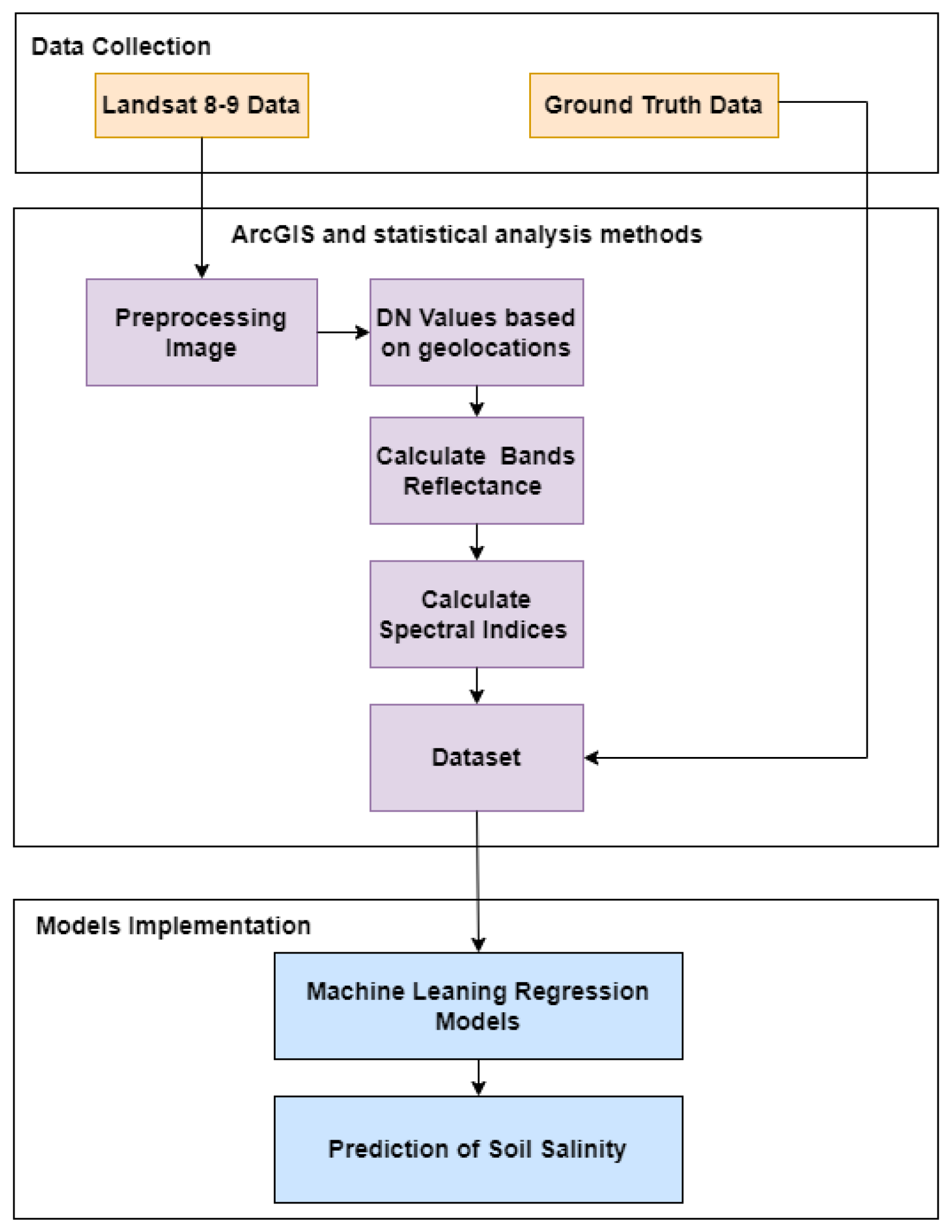
2. Material and Method

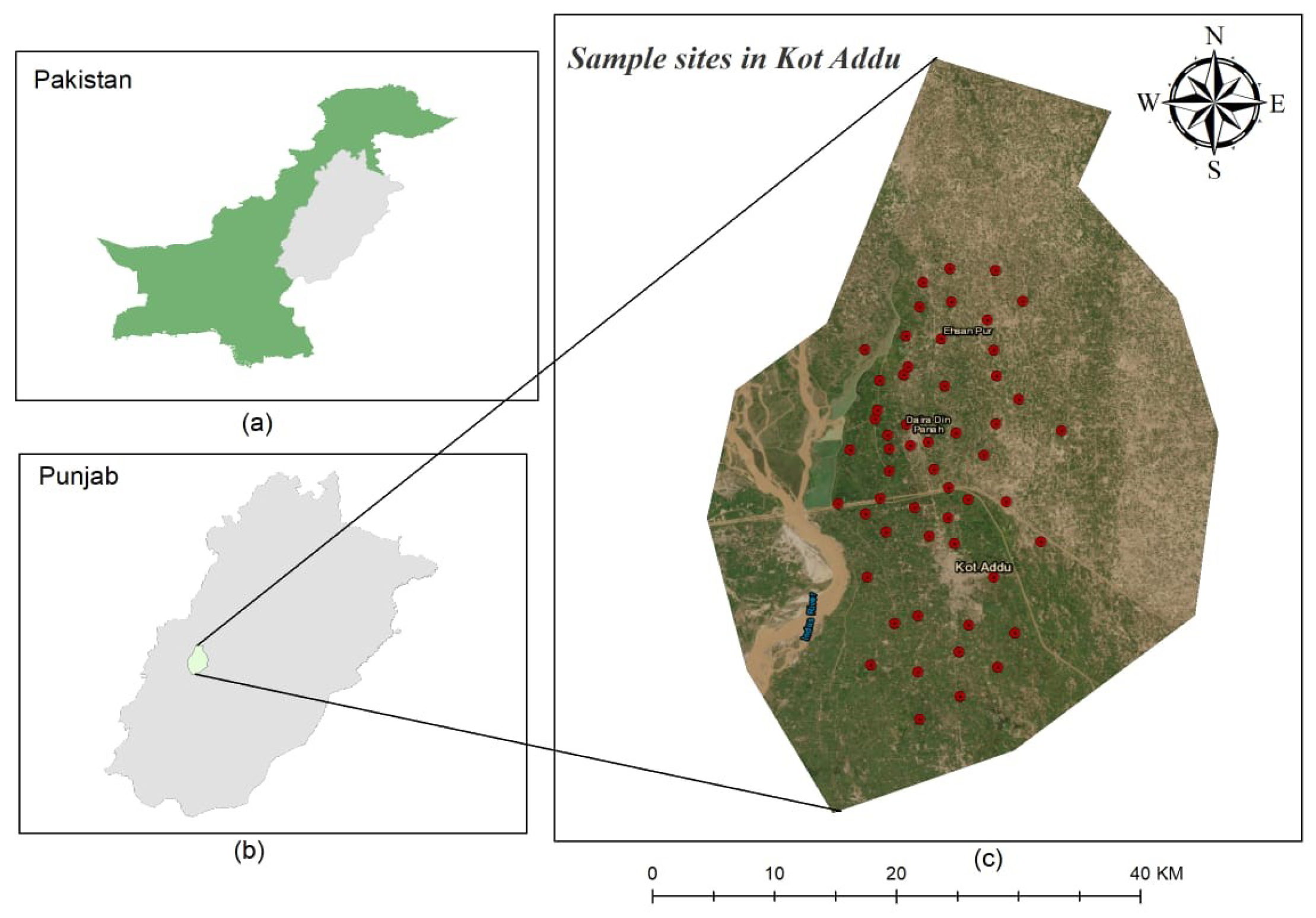
2.1. Study Area

Kot Addu city is situated in the center of Pakistan, in the southern region of the Punjab Province, in the District of Muzaffargarh Figure 1. Sugarcane, wheat and cotton are the principal crops farmed in the alluvial plain that surrounds the city; rice, maize, mash, ground nuts, bajra and oil seeds (rapeseed) are cultivated in a very small ratio. Frequently, certain areas remain flooded. Mangoes, citrus, dates and pomegranates are the principal fruit trees grown; however, many citrus and mango farms also have a small amount of space for pears, dates and bananas [43]. Most of the agricultural lands in this region are mildly to moderately salinized. Kot Addu experiences mild winter and scorching summer seasons due to its desert climate. The city has encountered some of the most severe climate conditions in Pakistan. The peak temperature ever noted was roughly 51 °C (324.15 °K), and the lowest temperature ever noted was roughly −1 °C (272.15 °K). About 127 mm of rain falls every year on average (5.0 in.). Such a climate exacerbates the salinity issue; therefore, research is being conducted to track the salinity issue in this region.

2.2. Satellite Data

The Landsat 8 data used in this study was obtained from January 10 to 30, 2017. Images with a cloud cover of less than 5 percent were exclusively chosen. Spectral indices were calculated utilizing spectral band values, as shown in

Table 1. Spectral indices for current study.

Spectral Indices	Expression	Reference
Normalized Difference Vegetation Index (NDVI)	$\frac{(NIR-R)}{(NIR+R)}$	[44]
Normalized Difference Salinity Index (NDSI)	$\frac{(R-NIR)}{(R+NIR)}$	[45]
Soil Adjusted Vegetation Index (SAVI)	$\frac{(NIR-R)}{(NIR+R)+L\ast (1-L)}$	[46]
Simple Ratio (SR)	$\frac{(R-NIR)}{(G+NIR)}$	[47]
Differential Vegetation Index (DVI)	$(NIR-R)$	[48]
Ratio Spectral Index (RSI)	$\frac{R}{NIR}$	[49]
Mosaic Simple Ratio (MSR)	$\frac{NIR}{R}$	[50]
Vegetation Soil Salinity Index (VSSI)	$2\ast G-5\ast (R+NIR)G-5\ast (R+NIR)$	[22]
Salinity Index (SI1)	$\frac{\left(B\right)}{\left(R\right)}$	[51]
Salinity Index (SI2)	$\frac{(B-R)}{B+R}$	[52]
Salinity Index (SI3)	$\frac{(G\ast R)}{B}$	[52]
Salinity Index (SI4)	$\frac{NIR\ast R}{G}$	[52]

. Band 8 panchromatic was excluded due to its proximity and susceptibility to cloud interference.

2.3. Soil Sample

To gather soil samples, a survey study was carried out by the Soil and Environmental Sciences Institute at Agriculture University Faisalabad in the Kot Addu region of the Muzaffargarh District in January 2017 [43]. The main objective was to monitor the salt status across the expansive 32,457-acre study area. A total of fifty-five soil samples were randomly collected from the top 15 cm of the soil surface using an auger. Geographical coordinates for each sample location were recorded using a GPS device. The collected soil samples were properly labeled, placed in polybags, and sent to the Soil and Water Testing Laboratory at the University of Agriculture, Faisalabad, for further analysis [43]. The soil specimens underwent grinding, air drying and filtration through a 2 mm sieve. The sieved soil was then transformed into a soil-saturated paste using purified water and left to rest overnight. The concentrated solution extracted from this paste was measured for electrical conductivity (EC) using a conductivity meter, to determine the soil EC [43].

2.4. Spectral Indices

Using Arc Map 10.3, twelve spectral indices were calculated from the preprocessed data based on the literature review [22,44,45,46,47,48,49,50,51,52]. The selection of these indices for the study was facilitated by their potential link to the detection of salinity.

The formulas for spectral indices are listed in Table 1.

After computing the spectral indices and forming the dataset, the subsequent step involved applying the standard scaler technique. This was carried out to ensure uniform contributions from the features before proceeding with the training of the machine learning models. The objective is to comprehend the association among satellite data (spectral indices) and the salt content of the soil specimens.

The methodology of the investigation represent in Figure 2.

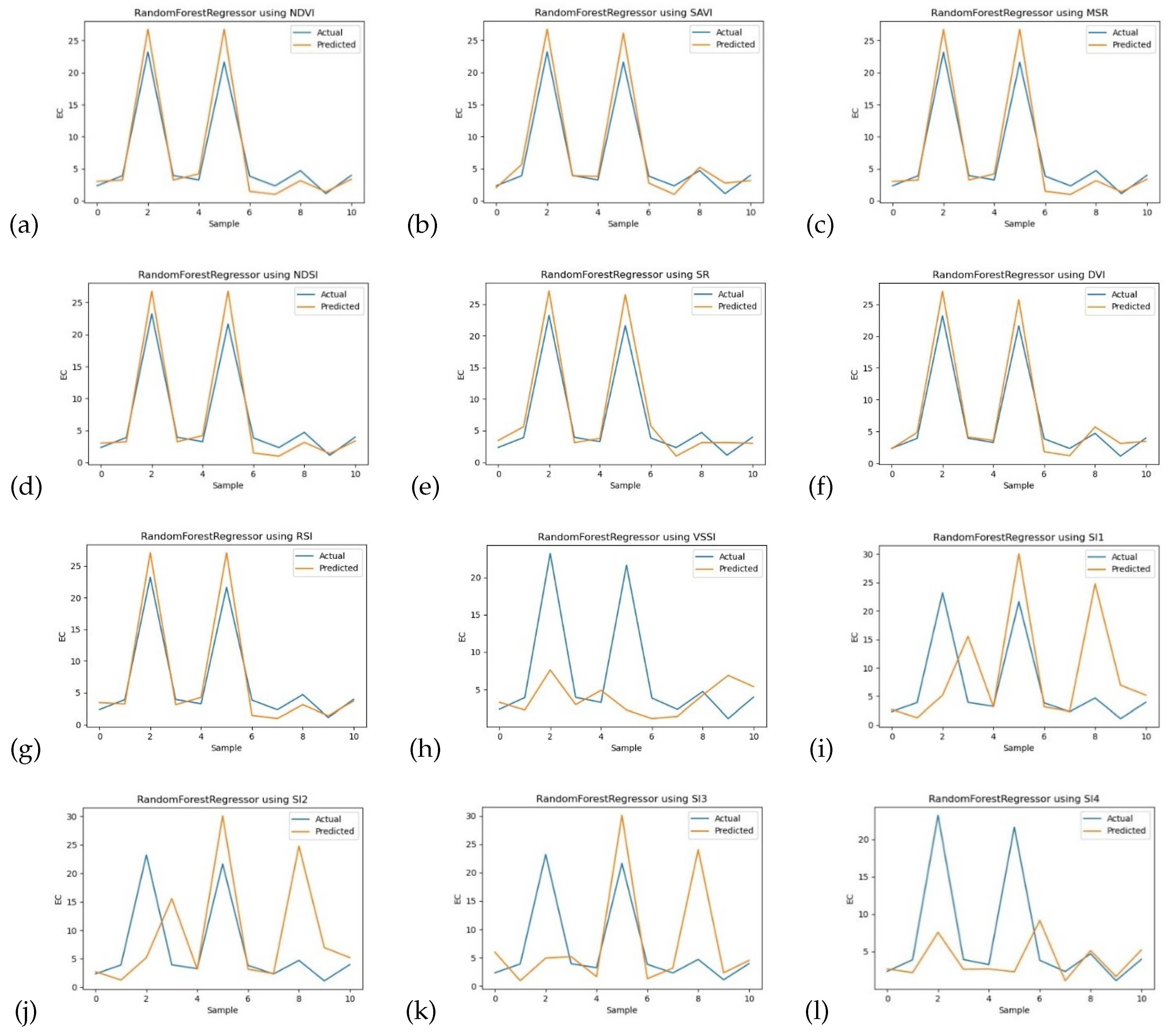
2.5. Random Forest Regressor

Breiman [53] and Cutler and Stevens [54] proposed an RF algorithm that works on the basis of several decision trees which are not correlated with each other [55]. It works as a classifier if labels are given, and like a regressor for continuous or numeric values. Random samples are selected from the calibration set to build the decision tree. For the complete division of variable space, random selections are made from n inputs to split each node in the decision tree. The average result of all decision trees is the final value of the RF model. Significant attention needs to be given to the tuning of the RF model for prediction, specifically in regards to the count of decision trees (ntree), the count of randomly sampled variables as candidates for each split (mtree) and the least count of specimens essential for a node to be considered a leaf (nodesize). The RF model is more stable, having a higher value of ntree. The nodesize value is determined by repeated testing (nodesize = 1). The The Residual Sum of Square (RSS) formula is used in the RFR model for regression. In this study, the RFR model is implemented by using the “RandomForestRegressor” from sklearn in jupyter notebook.

$$RSS=\sum _{left}{(y_i-y_L^{*})}^2+\sum _{right}{(y_i-y_R^{*})}^2$$

(1)

where $y_L^{*}$ is the mean y value for the left node and $y_R^{*}$ is the mean y value for the right node.

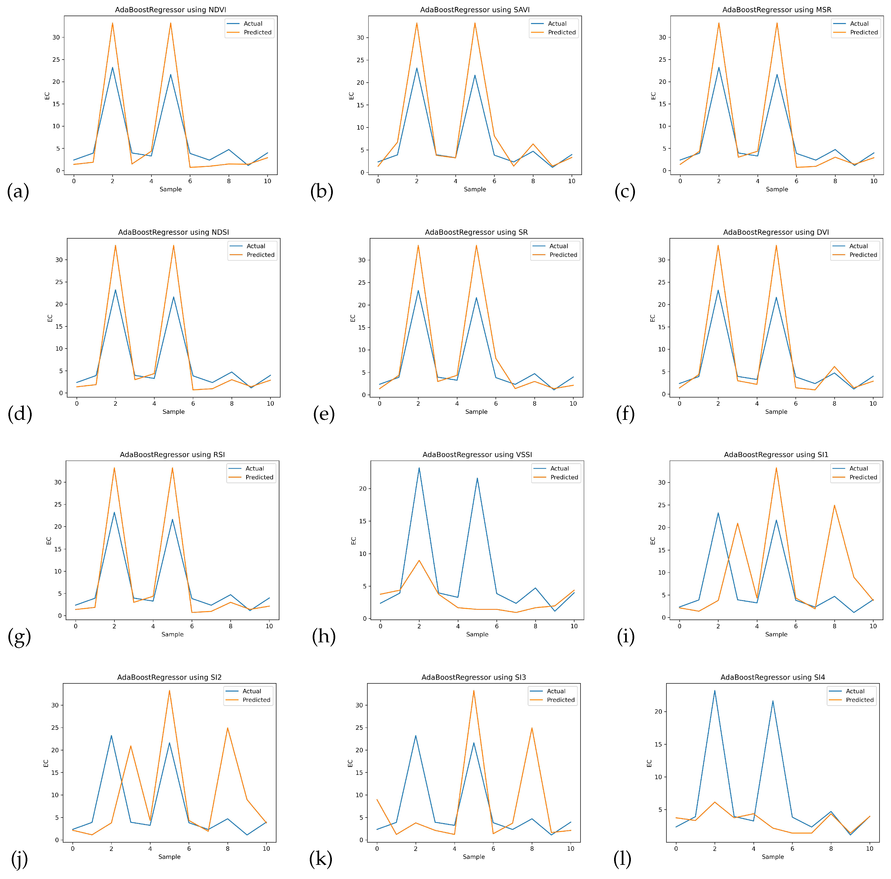
2.6. AdaBoost Regressor

AdaBoost, known as Adaptive Boosting, is an ensemble learning technique utilized for classification and regression tasks. For regression problems, it is referred to as AdaBoost Regressor. This widely used machine learning algorithm blends the predictions of several weak learners, typically shallow decision trees, to construct a robust ensemble model. The fundamental concept behind the ABR involves iteratively training a sequence of weak learners, with each subsequent learner emphasizing examples that previous ones struggled to predict accurately. This adaptive nature enables the model to enhance its performance through successive iterations.

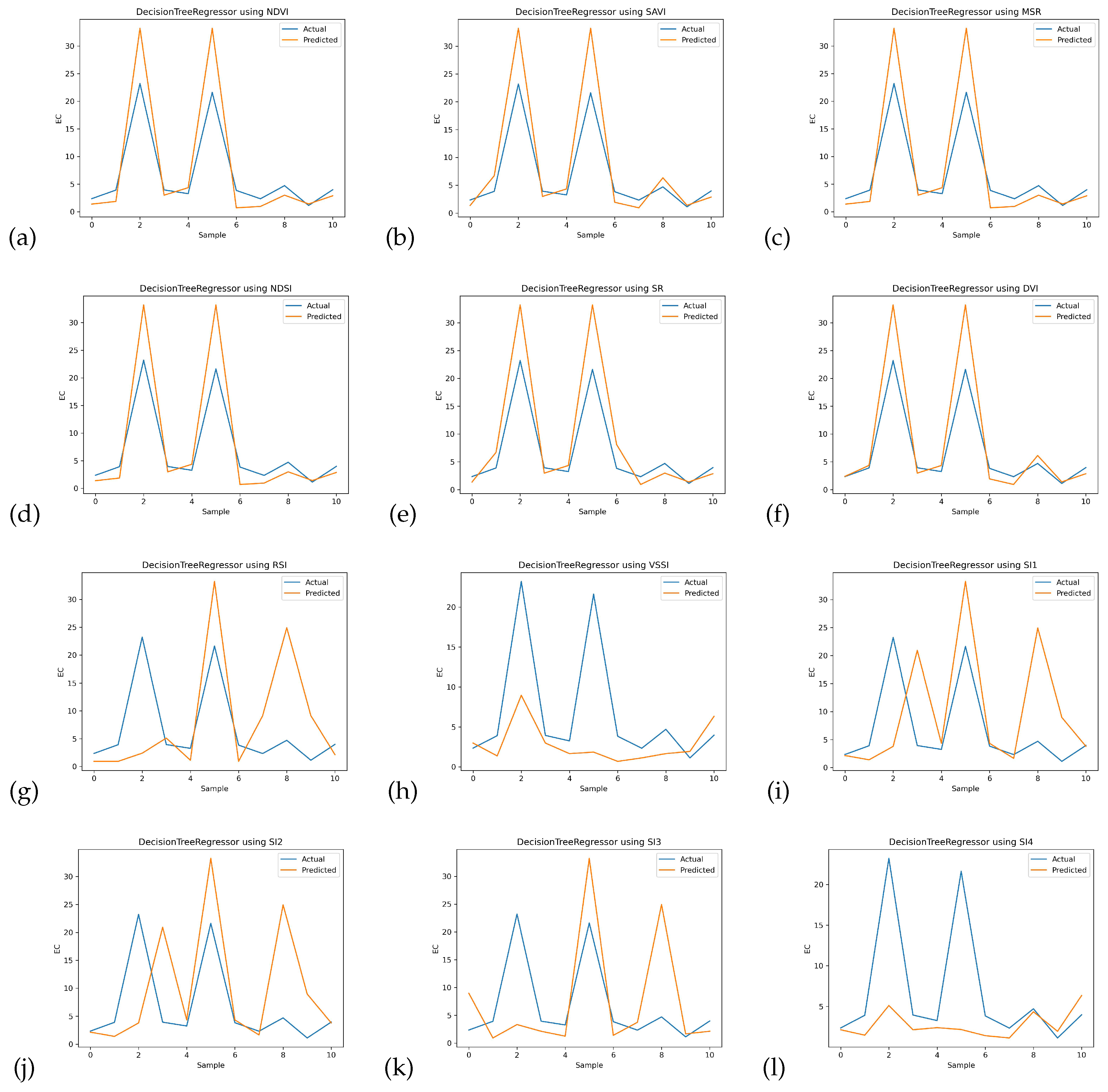
2.7. Decision Tree Regressor

The Decision Tree Regressor functions as a supervised machine learning technique utilized for regression purposes. Unlike classification challenges that seek to predict categorical labels, regression tasks focus on forecasting continuous numerical values. A decision tree takes the form of a tree-like model in which internal nodes indicate decisions based on specific features, while leaf nodes correspond to the predicted output values. In the case of the DTR, the value at each leaf node is derived from the average (or another measure) of the target values from the training samples that lead to that particular leaf.

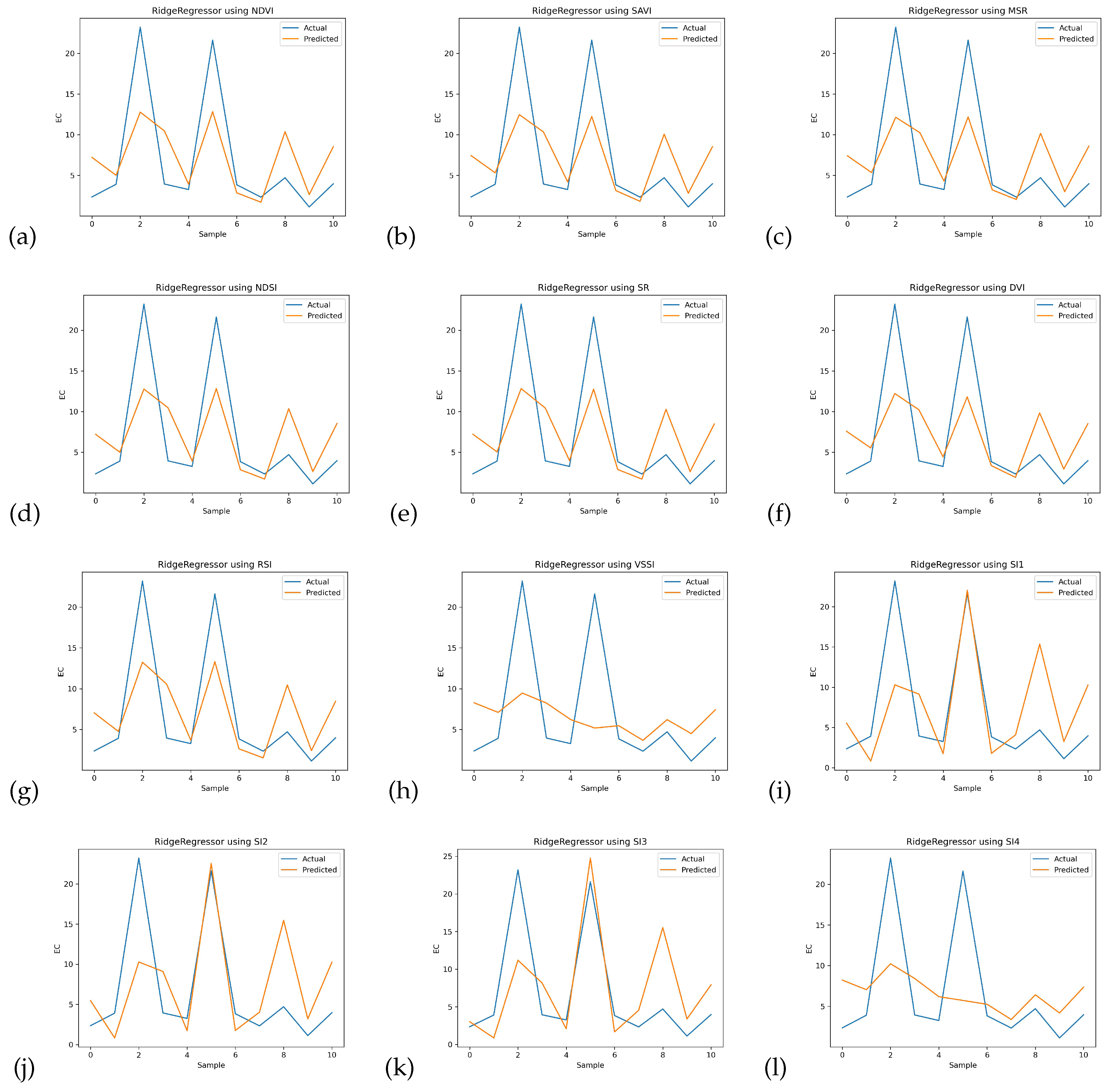
2.8. Ridge Regressor

The Ridge Regressor is a supervised linear regression algorithm, commonly employed in machine learning tasks, particularly when dealing with multicollinearity among predictor variables. It is a modified version of standard linear regression that incorporates a penalty term in the cost function to prevent overfitting and enhance generalization. In ordinary linear regression, the objective is to determine coefficients for predictor variables that minimize the sum of squared differences between predicted and actual target values. However, when predictor variables are highly correlated, the coefficients might grow large, leading to heightened sensitivity to noise and potential overfitting. To tackle this issue, the RR introduces an L2 regularization term to the linear regression cost function. This regularization term imposes a penalty based on the squared magnitudes of the coefficients. By applying this penalty, the RR encourages the model not only to fit the data but also to maintain small coefficients, effectively reducing the influence of individual predictors.

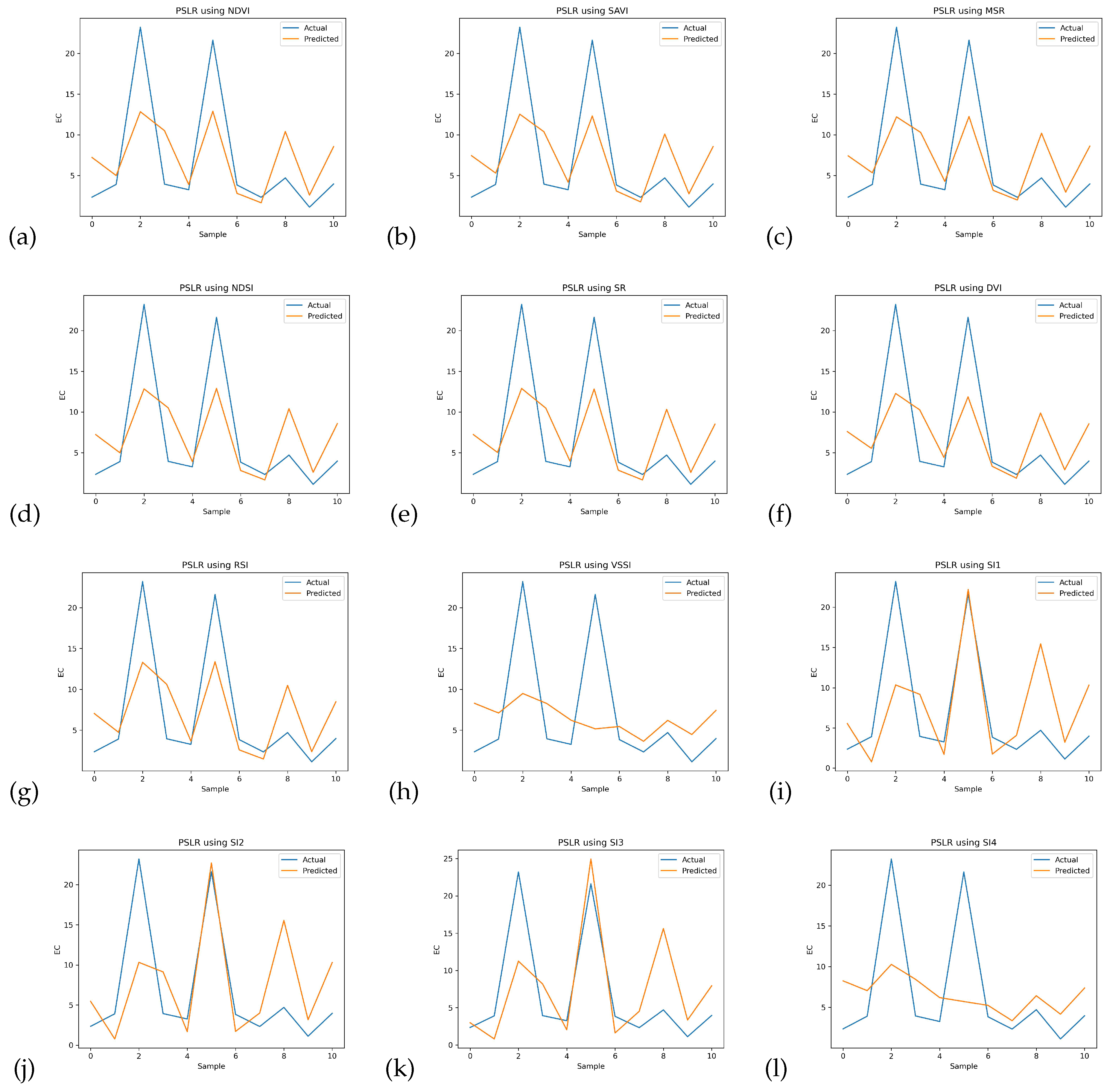
2.9. Partial Least Squares Regression

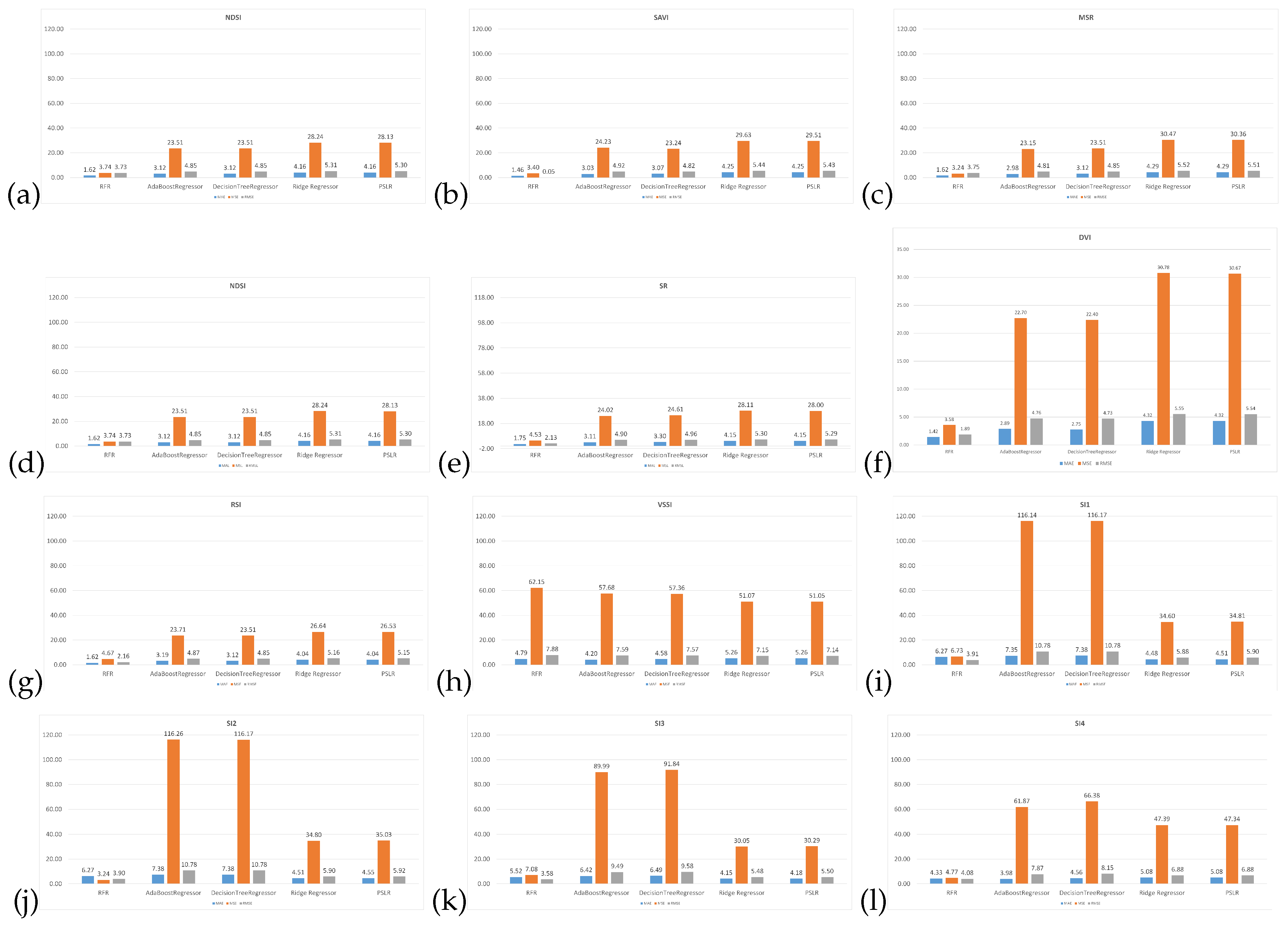
Partial Least Squares Regression is a statistical technique utilized to model the association between a group of independent variables (X) and a dependent variable (Y). It proves particularly valuable when working with datasets that exhibit high dimensionality or when there is a possibility of multicollinearity among the predictor variables. The primary objective of PLSR is to discover a reduced representation of both the independent and dependent variables by forming new latent variables (also called components) as linear combinations of the original variables. These components are crafted in a manner that maximizes the covariance between the independent and dependent variables within each subsequent component.

2.10. Evaluation

The regression algorithms received spectral indices as input, with the observed soil salinity serving as the target value. Overall, 55 soil specimens were gathered between January 20 and 27 January 2017. The dataset was then distributed into training and testing sets, with a proportion of 80% for calibration and 20% for validation. Out of the 55 samples, 45 were utilized for training the model, while the remaining 10 were used for testing. Various statistical parameters, including the R², MAE, MSE, and RMSE, were employed to assess the proficiency of the ML techniques.

$$R^2=1-\frac{{\sum }_{k=1}^n{(y_k-{\widehat{y}}_k)}^2}{{\sum }_{k=1}^n{(y_k-{\overline{y}}_k)}^2}$$

(2)

$$MAE=\frac{1}{n}\sum _{k=1}^n|y_k-{\widehat{y}}_k|$$

(3)

$$MSE=\frac{1}{n}\sum _{k=1}^n{(y_k-{\widehat{y}}_k)}^2$$

(4)

$$RMSE=\sqrt{\frac{1}{n}\sum _{k=1}^n{(y_k-{\widehat{y}}_k)}^2}$$

(5)

Here, $y_k$ is the kth observed salinity, ${\widehat{y}}_k$ is the kth predicted salinity, ${\overline{y}}_k$ is the mean salinity of all the soil samples, and n is the total count of specimens.

3. Results

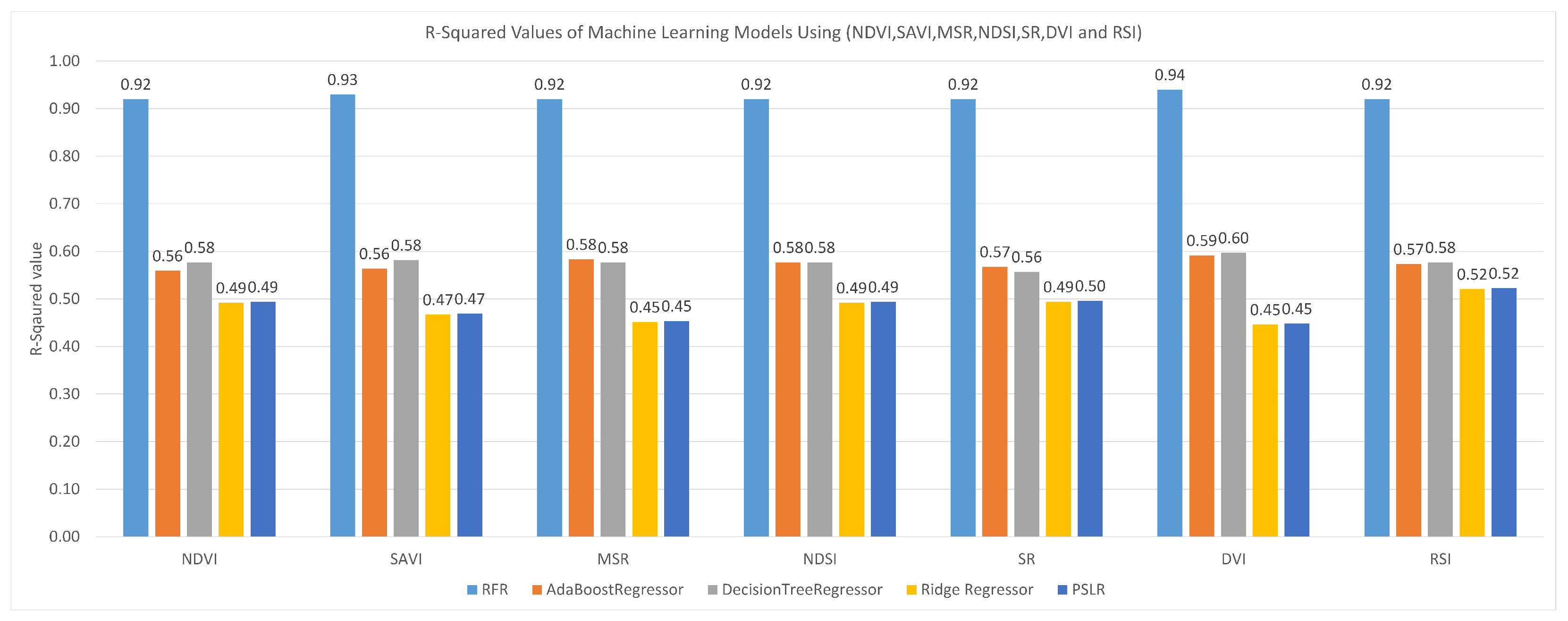
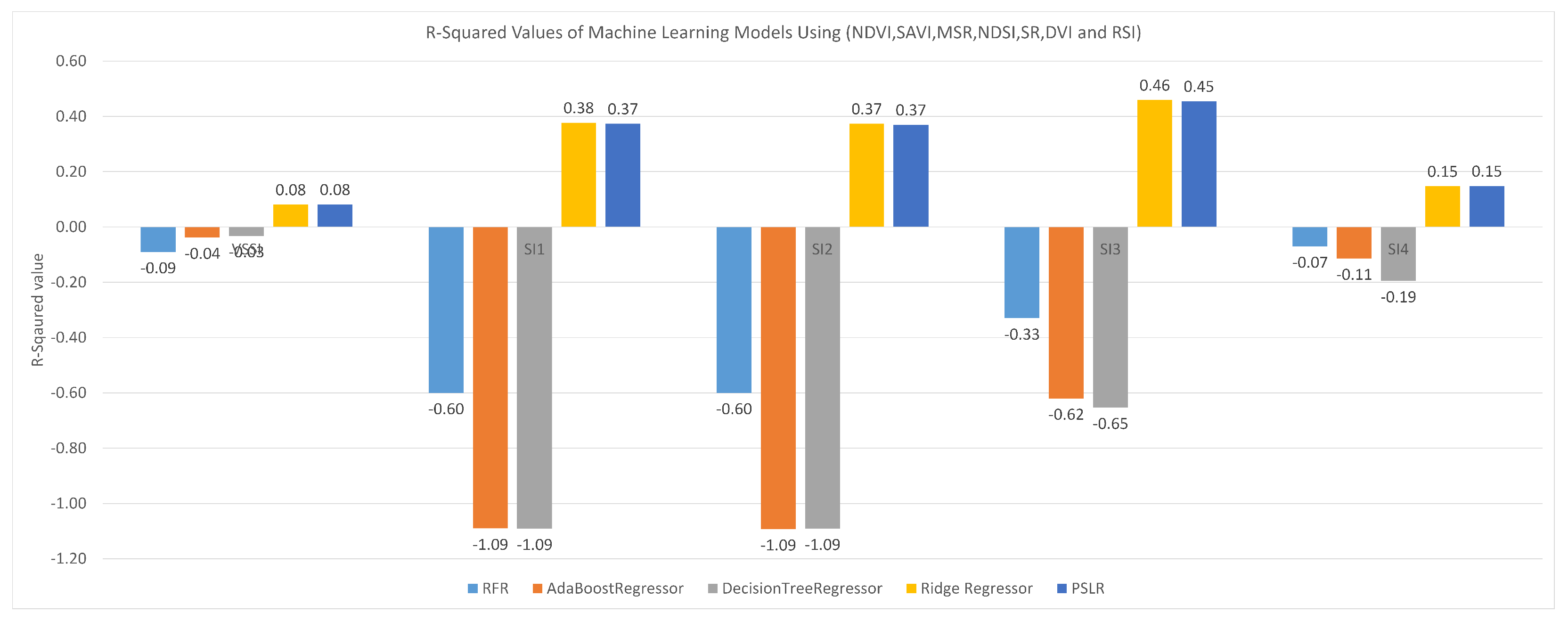
3.1. Models’ Performance

This study predicted the salinity of soil using spectral indices, and various statistical parameters, including the R², MAE, MSE and RMSE, were employed to assess the performance of ML models. Among these parameters, R² played a significant role in evaluating the model’s performance. It is a measure of how well the model has learned the data, and a higher R² value reveals a better fit of the model to the data. Twelve different spectral indices were used in the study, and their R² values were compared to determine which index is more efficient in mapping the salinity of soil. In Figure 3, a comprehensive analysis of R² values across a variety of spectral indices, including the NDVI, SAVI, MSR, NDSI, SR, DVI and RSI, is presented. The evaluation encompassed the utilization of multiple models, specifically the RFR, ADR, DTR, RR and PLSR. After a thorough analysis of the results, it becomes clear that the RFR model exhibited exceptional performance, particularly in relation to the DVI and SAVI spectral indices. Impressively, it achieved noteworthy R² values of 0.94 and 0.93 for these indices, respectively. In contrast, the implementation of the ADR model led to a distinct decline in R² values for these same indices, producing R² values of 0.59 and 0.56 for DVI and SAVI, respectively. Furthermore, the RFR model displayed superior R² values across several other spectral indices, including NDVI, MSR, NDSI, SR, and RSI, when compared to the ADR model. Conversely, the ADR model presented lower R² values for certain spectral indices like DTR, RR, and PLSR, when compared to the RFR model. As a result, the RFR model stands as a more suitable choice for accurately mapping soil salinity in this study. For a detailed account of the R² values for different spectral indices, refer to Figure 3.

The appropriate selection of spectral indices is crucial when mapping soil salinity using satellite data. Spectral indices play a fundamental role as input features for ML models in remote sensing applications. In the context of this study, the spectral indices VSSI, SI1, SI2, SI3 and SI4 displayed lower R² values, as depicted in Figure 4. These lower R² values indicate that, when utilizing these spectral indices as input features for the ML models, the models performed poorly, and their predictions did not closely match the actual soil salinity levels.

Figure 3. Comparison of R² of machine learning models using spectral indices NDVI, SAVI, MSR, NDSI, SR, DVI and RSI.

Figure 3. Comparison of R² of machine learning models using spectral indices NDVI, SAVI, MSR, NDSI, SR, DVI and RSI.

3.2. Model Calibration and Validation

For calibrating ML models using Landsat 8 OLI data, a total of twelve spectral indices were employed. The models were trained using 80% of the available samples, while the remaining 20% was used for testing. The implementation was carried out in Python, and four statistical methods (R², MAE, MSE and RMSE) were utilized to assess the models’ performance. The results presented in Figure 3 indicate that certain spectral indices, namely DVI, SAVI, NDVI, MSR, NDSI, SR and RSI, achieved high R² values, reflecting a strong correlation between the predictions made by the ML models and the actual soil salinity levels. On the contrary, Figure 5 reveals that specific spectral indices, such as VSSI, S1, S2, S3 and S4, produced very low R² values. These findings indicate that the ML models utilizing these indices were not effective in accurately predicting soil salinity levels, as their predictions did not closely match the actual data. Conversely, the exceptional performance of the RFR technique is particularly noteworthy, especially when integrating the DVI spectral index. The RFR model accomplished a significant R² value of 0.94, signifying a robust correlation between its predictions and the observed soil salinity levels. Furthermore, the model exhibited minimal errors with an MAE of 1.42, MSE of 3.58, and RMSE of 1.89. Collectively, these metrics emphasize the RFR model’s exceptional capability to precisely forecast soil salinity levels. Contrasting the error rates across various models using the DVI spectral index further highlights the superiority of the RFR model. The RFR model outperforms other models, illustrating notably reduced error rates in its soil salinity predictions, particularly when making use of the DVI spectral index. Remarkably, the RFR model attains an MAE of 1.42, an MSE of 3.58, and an RMSE of 1.89. In contrast, the ADR model shows higher error rates, presenting an MAE of 2.89, MSE of 22.70, and RMSE of 4.76. Similarly, the DTR and RR models demonstrate elevated errors, with MAE values of 2.75 and 4.32, along with corresponding MSE values of 22.40 and 30.78, respectively. Furthermore, the PLSR model exhibits comparable error rates to the RR model, featuring an MAE of 4.32, MSE of 30.67, and RMSE of 5.54. The significant difference in error rates between the RFR model and the alternative models highlights the RFR model’s superiority in precisely forecasting soil salinity, particularly when utilizing the DVI spectral index as an incorporated feature.

The line graphs depicting the RFR (Figure 6), ABR (Figure 7), DTR (Figure 8), RR (Figure 9), and PLSR (Figure 10) illustrate the visualization of the observed and estimated soil salinity values. On the x-axis, sample numbers are represented, while the y-axis displays both actual and predicted EC values, distinguished by different colors. Within the used spectral indices, encompassing DVI, SAVI, NDVI, MSR, NDSI, SR, and RSI, a close alignment is observed between the lines representing actual and predicted values in the line graphs. This close alignment indicates that these spectral indices yield better performance when used with the RFR model, resulting in more accurate predictions of soil salinity. On the other hand, spectral indices VSSI, SI1, SI2, SI3 and SI4 exhibit larger discrepancies between the actual and predicted lines in the line graphs. This observation suggests that these spectral indices are associated with higher error rates when analyzed with the RFR model, indicating that they may not be as effective in accurately predicting soil salinity. Overall, the visual analysis of the line graphs supports the finding that the RFR model, especially when utilizing distinct spectral indices, outperforms other ML models and offers more reliable predictions of soil salinity levels.

In Figure 6a–g, the predicted and actual lines using the RFR model are positioned closely together, indicating a strong alignment and accurate predictions. This finding suggests that certain spectral indices utilized in this section had lower error rates and resulted in the best model fit for predicting the salinity of soil. The close proximity of the lines in these graphs signifies that the model’s predictions closely match the actual soil salinity values, leading to more reliable results. However, a different scenario is observed in Figure 6i–l where spectral indices VSSI, SI1, SI2, SI3 and SI4 are used. In these graphs, the predicted and actual lines are more dispersed, indicating higher error rates and less accurate predictions by the RFR model. This outcome implies that, when mapping soil salinity, these specific spectral indices did not perform well in capturing the true salinity variations in the soil, resulting in less reliable predictions.

In Figure 7a–g, the predicted and observed lines obtained through the ABR model align closely when utilizing spectral indices such as the NDVI, SAVI, MSR, NDSI, SR, DVI and RSI. This alignment implies that these spectral indices demonstrate reduced error rates and yield more precise predictions for soil salinity mapping. The proximity of the lines in these graphs signifies the strong performance of the ABR model with these specific spectral indices, effectively capturing authentic salinity fluctuations within the soil and yielding dependable forecasts. Conversely, in Figure 7i–l, where the spectral indices VSSI, SI1, SI2, SI3 and SI4 are employed, the predicted and observed lines exhibit greater dispersion. This observation suggests elevated error rates associated with these spectral indices when employed for soil salinity mapping. The wider distribution of lines indicates that the ABR model’s efficacy with these indices is diminished, resulting in less precise predictions and increased uncertainties.

Figure 7. Line graphs of EC values using AdaBoost Regressor (a) NDVI, (b) SAVI, (c) MSR, (d) NDSI, (e) SR, (f) DVI, (g) RSI, (h) VSSI, (i) SI1, (j) SI2, (k) SI3, (l) SI4.

Figure 7. Line graphs of EC values using AdaBoost Regressor (a) NDVI, (b) SAVI, (c) MSR, (d) NDSI, (e) SR, (f) DVI, (g) RSI, (h) VSSI, (i) SI1, (j) SI2, (k) SI3, (l) SI4.

In Figure 8a–g, the predicted and actual lines using the DTR (Decision Tree Regression) model are not as closely aligned as those in Figure 6a–g, which indicates that the DTR model has higher error rates compared to the RFR (Random Forest Regression) model when predicting soil salinity. The spread between the predicted and actual lines in Figure 8a–g suggests that the DTR model did not perform as well as the RFR model, leading to less accurate predictions and higher uncertainties. However, when comparing the DTR model (Figure 8) to the RR model (Figure 9) and the PLSR model (Figure 10), the predicted and actual lines are closer. This observation indicates that the DTR model has lower error rates compared to the RR and PLSR models when using the same spectral indices for predicting soil salinity.

Figure 8. Line graphs of EC values using Decision Tree Regressor (a) NDVI, (b) SAVI, (c) MSR, (d) NDSI, (e) SR, (f) DVI, (g) RSI, (h) VSSI, (i) SI1, (j) SI2, (k) SI3, (l) SI4.

Figure 8. Line graphs of EC values using Decision Tree Regressor (a) NDVI, (b) SAVI, (c) MSR, (d) NDSI, (e) SR, (f) DVI, (g) RSI, (h) VSSI, (i) SI1, (j) SI2, (k) SI3, (l) SI4.

When comparing the predicted and actual lines of the PLSR model (Figure 10) to those of the RFR (Figure 6), ABR (Figure 7) and DTR (Figure 8) models, the gap is more pronounced. This visual analysis underscores that the PLSR model exhibits the highest error rate among the models under consideration. The comparative evaluation of line graphs underscores that the PLSR model is characterized by elevated error rates and less accurate predictions compared to the other models.

Figure 9. Line graphs of EC values using Ridge Regressor (a) NDVI, (b) SAVI, (c) MSR, (d) NDSI, (e) SR, (f) DVI, (g) RSI, (h) VSSI, (i) SI1, (j) SI2, (k) SI3, (l) SI4.

Figure 9. Line graphs of EC values using Ridge Regressor (a) NDVI, (b) SAVI, (c) MSR, (d) NDSI, (e) SR, (f) DVI, (g) RSI, (h) VSSI, (i) SI1, (j) SI2, (k) SI3, (l) SI4.

Figure 10. Line graphs of EC values using Partial Least Square Regressor (a) NDVI, (b) SAVI, (c) MSR, (d) NDSI, (e) SR, (f) DVI, (g) RSI, (h) VSSI, (i) SI1, (j) SI2, (k) SI3, (l) SI4.

Figure 10. Line graphs of EC values using Partial Least Square Regressor (a) NDVI, (b) SAVI, (c) MSR, (d) NDSI, (e) SR, (f) DVI, (g) RSI, (h) VSSI, (i) SI1, (j) SI2, (k) SI3, (l) SI4.

4. Discussion

The first research objective was to assess the accuracy of predicting soil salinity using Landsat 8 OLI data with the aid of ML models. We successfully achieved soil salinity predictions by employing these ML models in conjunction with various spectral indices. The RFR model performed exceptionally well with an R² of 0.93 (Figure 3), MAE of 1.46, MSE of 3.90 and RMSE of 1.97 when using the SAVI spectral index as shown in (Figure 5). However, upon further analysis, we found that the RFR model provided even more precise predictions with an R² of 0.94 (Figure 3), MAE of 1.42, MSE of 3.58 and RMSE of 1.89 when utilizing the DVI spectral index (Figure 5). The predicted and actual lines using the RFR model were closely aligned in Figure 6f, indicating the model’s strong performance in accurately predicting soil salinity. Conversely, when using the SAVI spectral index, the ADT model exhibited higher error rates with an R² of 0.56, MAE of 3.03, MSE of 24.23 and RMSE of 4.92. However, the ADT model showed improved predictions with an R² of 0.59, MAE of 2.89, MSE of 22.70 and RMSE of 4.76 when utilizing the DVI spectral index. Similarly, the DTR model revealed increased error rates, presenting an R² value of 0.58, a MAE of 3.07, an MSE of 23.24 and an RMSE of 4.82 when making use of the SAVI spectral index. On the other hand, the DTR model illustrated enhanced performance, achieving an R² of 0.59, a MAE of 2.75, an MSE of 22.40 and an RMSE of 4.73 through the utilization of the DVI spectral index. In contrast, the RR model demonstrated diminished R² values and elevated error rates, indicating a suboptimal fit when employing the SAVI spectral index, resulting in an R² of 0.47, a MAE of 4.25, an MSE of 29.63 and an RMSE of 5.44. A slight improvement in results was noted as the RR model integrated the DVI spectral index, resulting in an R² value of 0.47, a MAE of 4.25, an MSE of 29.63, and an RMSE of 5.44. Similarly, the utilization of the SAVI spectral index by the PLSR model led to higher error rates, yielding an R² of 0.47, a MAE of 4.25, an MSE of 29.51, and an RMSE of 5.43. A slight increase in error rates was observed when the PLSR model applied the DVI spectral index, resulting in an R² of 0.47, an MAE of 4.32, an MSE of 30.67 and an RMSE of 5.54.

Conversely, when utilizing the VSSI, SI1, SI2, SI3, and SI4 spectral indices for soil salinity prediction, the ML models exhibited high error rates and notably low R² values. These outcomes clearly indicated that these specific spectral indices were not well-suited for the models and they had significant errors in predicting the actual salinity values, as depicted in Figure 4. The large discrepancies between the forecast and real salinity values for these spectral indices suggest that they may not capture the essential information needed for accurate soil salinity predictions, highlighting the importance of careful selection of appropriate spectral indices for improving model performance. The RFR model outperformed the ADR, DTR, RR and PLSR models due to its implementation of random sampling [55], superior fitting on small datasets [56] and consequent enhancement in decision-making accuracy [54]. Overall, the RFR model outperformed the other models in predicting soil salinity, especially when using the DVI spectral index. The selection of appropriate spectral indices is crucial in optimizing the performance of the ML models for accurate soil salinity predictions.

The second research objective aimed to identify the most efficient spectral indices for mapping the salinity of soil using Landsat 8 OLI data. For this purpose, twelve spectral indices were employed for mapping the salinity of soil. Higher R² values and minimum error rates were found during the prediction of salinity of soil by seven specific spectral indices (DVI, SAVI, NDVI, NDSI, MSR, SR, and RSI). Likewise, notable correlation between NDSI, NDVI, and SAVI indices to the level of salinity of soil was revealed in preliminary analysis [38]. More importantly, a unique demonstration of performance was made by DVI index with an impressive R² value of 0.94. Moreover, it demonstrated outstanding accuracy in predicting the salinity of soil with the minimal values of MAE of 1.42, an MSE of 3.58, and an RMSE of 1.89 (Figure 6f). This underscores its strong alignment with the RFR model and its significant contribution to precise soil salinity predictions. The findings indicated that spectral indices utilizing the NIR band [37] displayed greater accuracy in predicting soil salinity compared to those relying on visible bands. In contrast, the VSSI, SI1, SI2, SI3 and SI4 indices exhibited lower R² values (Figure 4) and higher error rates (Figure 4), indicating their reduced effectiveness in accurately estimating soil salinity.

The third research objective was to identify the most efficient ML model for determining the salinity of soil using Landsat 8 OLI data. The performance of five ML techniques were compared based on R², MAE, MSE and RMSE metrics. The results clearly demonstrated that the RFR model, specifically using the DVI index, outperformed the other ML models, including the ABR, DTR, RR and PLSR, when using the selected spectral indices (excluding VSSI, SI1, SI2, SI3 and SI4) from Landsat 8 OLI data to forecast the salinity of soil. The RFR model achieved an impressive R² of 0.94, indicating a strong correlation between predicted and observed soil salinity values, and exhibited minimum error rates as depicted in Figure 3. When comparing the predicted and actual salinity lines, the RFR model (Figure 6) demonstrated a closer alignment, highlighting its superior performance compared to the ABR (Figure 7), DTR (Figure 8), RR (Figure 9) and PLSR (Figure 10) models. This indicates that the RFR model provided more accurate predictions and better captured the variations in soil salinity, making it the most efficient ML model for this specific task [54,55]. These findings emphasize the significance of selecting an appropriate ML algorithm and spectral indices when mapping soil salinity using satellite data, as it directly impacts the accuracy and reliability of the predictions.

This study makes a valuable addition to the application of ML models for the mapping of salinity of soil based on spectral indices, because we have successfully predicted the salinity of soil by Landsat 8 imagery with the highest 0.94 of R². We can determine the soil salinity of barren land by just entering the geo-coordinates. It can be useful to predict the soil salinity of barren land in Pakistan and the global region. If the soil salinity of the land is determined in time, then we can take necessary steps to decrease the soil erosion. The proper soil salinity value (EC < 4) has a significant impact on the growth of the plants. The soil salinity level is an important factor in deciding the suitable crop for cultivation on a specific plot of land. So, this study helps to improve agriculture management practices.

5. Conclusions

The salinity of soil is a significant global issue, notably in arid and semiarid regions, and it poses detrimental effects on food security worldwide. It deteriorates the soil environment and has adverse impacts on climate, hydrology, agriculture, geochemistry and the economy. Regular monitoring of the scale and intensity of soil salinity is crucial to mitigate these environmental risks. Hence, remote sensing presents a suitable option for remotely determining the salinity of soil in specific regions. The current study demonstrates the effectiveness of Landsat 8 OLI data, specifically spectral indices, in characterizing and evaluating soil salinity. Satellite data reveal that saline soils exhibit higher reflectance in the visible, NIR and SWIR spectra compared to regular soils. While salinity indices SI1, SI2, SI3 and SI4 are not useful in vegetated regions, they can be employed for comprehensive observations and the assessment of saline soils. Among the five ML models utilized for estimating the salinity of soil derived from spectral indices, the RFR model demonstrated the best performance in evaluating salinity in study area with an R² 0.94, MAE 1.42, MSE 3.58 and RMSE 1.89 as compared to ADB, DTR, RR and PLSR. Among the twelve spectral indices utilized, DVI, SAVI, NDVI, NDSI, MSR, SR and RSI exhibited significant correlations with soil salinity. These indices are recommended to spatially map the salinity of soil. On the other hand, VSSI, SI1, SI2, SI3 and SI4 had unclear correlations with the salinity of soil. Based on the results, it is possible to develop a web-based application that allows users to map soil salinity by entering the geocoordinates. Such an application would be beneficial for farmers and agricultural management, enabling them to make informed decisions regarding crop selection to mitigate monetary losses caused by climate change. This method offers a cost-effective and efficient approach for detecting soil salinity in specific regions. Furthermore, since Landsat 8 OLI data are freely available, the results of this study can be optimized by increasing the dataset and applying deep learning models.

References

1. Lhissoui, R.; El Harti, A.; Chokmani, K. Mapping soil salinity in irrigated land using optical remote sensing data. Eurasian J. Soil Sci. 2014, 3, 82–88. [Google Scholar]
2. Asfaw, E.; Suryabhagavan, K.; Argaw, M. Soil salinity modeling and mapping using remote sensing and GIS: The case of Wonji sugar cane irrigation farm, Ethiopia. J. Saudi Soc. Agric. Sci. 2018, 17, 250–258. [Google Scholar] [CrossRef]
3. FAO. Extent and Causes of Salt Affected Soils in Participating Countries. Global Network on Integrated Soil Management for Sustainable Use of Saltaffected Soils. 2000. Available online: http://www.fao.org/ag/agl/agll/spush/topic2.htm (accessed on 22 May 2023).
4. Zhu, J.K. Plant salt tolerance. Trends Plant Sci. 2001, 6, 66–71. [Google Scholar]
5. Metternicht, G.I.; Zinck, J. Remote sensing of soil salinity: Potentials and constraints. Remote Sens. Environ. 2003, 85, 1–20. [Google Scholar]
6. Zheng, Z.; Zhang, F.; Ma, F.; Chai, X.; Zhu, Z.; Shi, J.; Zhang, S. Spatiotemporal changes in soil salinity in a drip-irrigated field. Geoderma 2009, 149, 243–248. [Google Scholar] [CrossRef]
7. Yao, R.; Yang, J. Quantitative evaluation of soil salinity and its spatial distribution using electromagnetic induction method. Agric. Water Manag. 2010, 97, 1961–1970. [Google Scholar] [CrossRef]
8. Scudiero, E.; Corwin, D.; Anderson, R.; Yemoto, K.; Clary, W.; Wang, Z.; Skaggs, T. Remote sensing is a viable tool for mapping soil salinity in agricultural lands. Calif. Agric. 2017, 71, 231–238. [Google Scholar] [CrossRef]
9. Bilgili, A.V.; Cullu, M.A.; van Es, H.; Aydemir, A.; Aydemir, S. The use of hyperspectral visible and near infrared reflectance spectroscopy for the characterization of salt-affected soils in the Harran Plain, Turkey. Arid Land Res. Manag. 2011, 25, 19–37. [Google Scholar]
10. Brunner, P.; Li, H.; Kinzelbach, W.; Li, W. Generating soil electrical conductivity maps at regional level by integrating measurements on the ground and remote sensing data. Int. J. Remote Sens. 2007, 28, 3341–3361. [Google Scholar] [CrossRef]
11. Dehaan, R.; Taylor, G. Image-derived spectral endmembers as indicators of salinisation. Int. J. Remote Sens. 2003, 24, 775–794. [Google Scholar] [CrossRef]
12. Nanni, M.R.; Demattê, J.A.M. Spectral reflectance methodology in comparison to traditional soil analysis. Soil Sci. Soc. Am. J. 2006, 70, 393–407. [Google Scholar] [CrossRef]
13. Haq, Y.U.; Shahbaz, M.; Asif, H.S.; Al-Laith, A.; Alsabban, W.; Aziz, M.H. Identification of soil type in Pakistan using remote sensing and machine learning. PeerJ Comput. Sci. 2022, 8, e1109. [Google Scholar]
14. Ramzan, Z.; Asif, H.S.; Yousuf, I.; Shahbaz, M. A Multimodal Data Fusion and Deep Neural Networks Based Technique for Tea Yield Estimation in Pakistan Using Satellite Imagery. IEEE Access 2023, 11, 42578–42594. [Google Scholar] [CrossRef]
15. Farifteh, J.; Farshad, A.; George, R. Assessing salt-affected soils using remote sensing, solute modelling, and geophysics. Geoderma 2006, 130, 191–206. [Google Scholar]
16. Liu, Y.; Zhang, F.; Wang, C.; Wu, S.; Liu, J.; Xu, A.; Pan, K.; Pan, X. Estimating the soil salinity over partially vegetated surfaces from multispectral remote sensing image using non-negative matrix factorization. Geoderma 2019, 354, 113887. [Google Scholar] [CrossRef]
17. Dale, P.; Hulsman, K.; Chandica, A. Classification of reflectance on colour infrared aerial photographs and sub-tropical salt-marsh vegetation types. Int. J. Remote Sens. 1986, 7, 1783–1788. [Google Scholar] [CrossRef]
18. ten Caten, A.; Dalmolin, R.S.D.; de Araujo Pedron, F.; Santos, M.d.L.M. Principal components as predictor variables in digital mapping of soil classes/Componentes principais como preditores no mapeamento digital de classes de solos. Ciência Rural 2011, 41, 1170–1177. [Google Scholar] [CrossRef]
19. Sahu, S.; Prasad, M.; Tripathy, B. PCA Classification technique of remote sensing analysis of colour composite image of chillika lagoon, Odisha. Int. J. Adv. Res. Comput. Sci. Softw. Eng. 2015, 5, 513–518. [Google Scholar]
20. Li, B.; Ti, C.; Zhao, Y.; Yan, X. Estimating soil moisture with Landsat data and its application in extracting the spatial distribution of winter flooded paddies. Remote Sens. 2016, 8, 38. [Google Scholar] [CrossRef]
21. Wu, W. The generalized difference vegetation index (GDVI) for dryland characterization. Remote Sens. 2014, 6, 1211–1233. [Google Scholar] [CrossRef]
22. Dehni, A.; Lounis, M. Remote sensing techniques for salt affected soil mapping: Application to the Oran region of Algeria. Procedia Eng. 2012, 33, 188–198. [Google Scholar] [CrossRef]
23. van Leeuwen, W.J. Visible, near-IR, and shortwave IR spectral characteristics of terrestrial surfaces. In The SAGE Handbook of Remote Sensing; Sage Publications Ltd.: New York, NY, USA, 2009. [Google Scholar]
24. Aceves, E.Á.; Guevara, H.J.P.; Enríquez, A.C.; Gaxiola, J.; Cervantes, M.; Barrientos, J.H.; Herrera, L.E.; Guevara, V.M.P.; Samuel, C.L. Determining salinity and ion soil using satellite image processing. Pol. J. Environ. Stud. 2019, 28, 1549–1560. [Google Scholar] [CrossRef]
25. Ling, C.; Liu, H.; Ju, H.; Zhang, H.; You, J.; Li, W. A study on spectral signature analysis of wetland vegetation based on ground imaging spectrum data. J. Physics Conf. Ser. 2017, 910, 12045. [Google Scholar] [CrossRef]
26. Ji, W.; Adamchuk, V.; Chen, S.; Biswas, A.; Leclerc, M.; Rossel, R.V. The use of proximal soil sensor data fusion and digital soil mapping for precision agriculture. Pedometrics 2017, 2017, 298. [Google Scholar]
27. Li, Z.; Li, Y.; Xing, A.; Zhuo, Z.; Zhang, S.; Zhang, Y.; Huang, Y. Spatial prediction of soil salinity in a semiarid oasis: Environmental sensitive variable selection and model comparison. Chin. Geogr. Sci. 2019, 29, 784–797. [Google Scholar] [CrossRef]
28. Pandey, P.; Singh, S.; Khan, M.S.; Semwal, M. Non-invasive Estimation of Foliar Nitrogen Concentration Using Spectral Characteristics of Menthol Mint (Mentha arvensis L.). Front. Plant Sci. 2022, 13, 680282. [Google Scholar] [CrossRef]
29. El Hafyani, M.; Essahlaoui, A.; El Baghdadi, M.; Teodoro, A.C.; Mohajane, M.; El Hmaidi, A.; El Ouali, A. Modeling and mapping of soil salinity in Tafilalet plain (Morocco). Arab. J. Geosci. 2019, 12, 1–7. [Google Scholar] [CrossRef]
30. Hihi, S.; Rabah, Z.B.; Bouaziz, M.; Chtourou, M.Y.; Bouaziz, S. Prediction of soil salinity using remote sensing tools and linear regression model. Adv. Remote Sens. 2019, 8, 77–88. [Google Scholar] [CrossRef]
31. Ivushkin, K.; Bartholomeus, H.; Bregt, A.K.; Pulatov, A. Satellite thermography for soil salinity assessment of cropped areas in Uzbekistan. Land Degrad. Dev. 2017, 28, 870–877. [Google Scholar] [CrossRef]
32. Hoa, P.V.; Giang, N.V.; Binh, N.A.; Hai, L.V.H.; Pham, T.D.; Hasanlou, M.; Tien Bui, D. Soil salinity mapping using SAR Sentinel-1 data and advanced machine learning algorithms: A case study at Ben Tre Province of the Mekong River Delta (Vietnam). Remote Sens. 2019, 11, 128. [Google Scholar] [CrossRef]
33. Taghadosi, M.M.; Hasanlou, M.; Eftekhari, K. Soil salinity mapping using dual-polarized SAR Sentinel-1 imagery. Int. J. Remote Sens. 2019, 40, 237–252. [Google Scholar] [CrossRef]
34. Zurqani, H.; Nwer, B.; Rhoma, A. Assessment of spatial and temporal variations of soil salinity using remote sensing and geographic information system in Libya. In Proceedings of the 1st Annual International Conference on Geological and Earth Sciences, Singapore, 3–4 December 2012; pp. 3–4. [Google Scholar]
35. Yong-Ling, W.; Peng, G.; Zhi-Liang, Z. A spectral index for estimating soil salinity in the Yellow River Delta Region of China using EO-1 Hyperion data. Pedosphere 2010, 20, 378–388. [Google Scholar]
36. Sahbeni, G. Soil salinity mapping using Landsat 8 OLI data and regression modeling in the Great Hungarian Plain. SN Appl. Sci. 2021, 3, 587. [Google Scholar] [CrossRef]
37. Al-Ali, Z.; Bannari, A.; Rhinane, H.; El-Battay, A.; Shahid, S.A.; Hameid, N. Validation and comparison of physical models for soil salinity mapping over an arid landscape using spectral reflectance measurements and Landsat-OLI data. Remote Sens. 2021, 13, 494. [Google Scholar] [CrossRef]
38. Zhang, X.; Huang, B. Prediction of soil salinity with soil-reflected spectra: A comparison of two regression methods. Sci. Rep. 2019, 9, 5067. [Google Scholar] [CrossRef]
39. Alhammadi, M.; Glenn, E. Detecting date palm trees health and vegetation greenness change on the eastern coast of the United Arab Emirates using SAVI. Int. J. Remote Sens. 2008, 29, 1745–1765. [Google Scholar] [CrossRef]
40. Iqbal, F. Detection of salt affected soil in rice-wheat area using satellite image. Afr. J. Agric. Res. 2011, 6, 4973–4982. [Google Scholar]
41. Zhang, T.T.; Zeng, S.L.; Gao, Y.; Ouyang, Z.T.; Li, B.; Fang, C.M.; Zhao, B. Using hyperspectral vegetation indices as a proxy to monitor soil salinity. Ecol. Indic. 2011, 11, 1552–1562. [Google Scholar] [CrossRef]
42. Aldakheel, Y.Y. Assessing NDVI spatial pattern as related to irrigation and soil salinity management in Al-Hassa Oasis, Saudi Arabia. J. Indian Soc. Remote Sens. 2011, 39, 171–180. [Google Scholar] [CrossRef]
43. Ijaz, M.; Ahmad, H.R.; Bibi, S.; Ayub, M.A.; Khalid, S. Soil salinity detection and monitoring using Landsat data: A case study from Kot Addu, Pakistan. Arab. J. Geosci. 2020, 13, 1–9. [Google Scholar] [CrossRef]
44. Rouse, J.W.; Haas, R.H.; Schell, J.A.; Deering, D.W. Monitoring vegetation systems in the Great Plains with ERTS. NASA Spec. Publ. 1974, 351, 309. [Google Scholar]
45. Khan, N.M.; Rastoskuev, V.V.; Sato, Y.; Shiozawa, S. Assessment of hydrosaline land degradation by using a simple approach of remote sensing indicators. Agric. Water Manag. 2005, 77, 96–109. [Google Scholar] [CrossRef]
46. Huete, A.R. A soil-adjusted vegetation index (SAVI). Remote Sens. Environ. 1988, 25, 295–309. [Google Scholar] [CrossRef]
47. Abbas, A.; Khan, S. Using remote sensing techniques for appraisal of irrigated soil salinity. In Proceedings of the International Congress on Modelling and Simulation (MODSIM), Christenchurch, New Zealand, 10–13 December 2007; Modelling and Simulation Society of Australia and New Zealand: Christenchurch, New Zealand, 2007; pp. 2632–2638. [Google Scholar]
48. Basso, F.; Bove, E.; Dumontet, S.; Ferrara, A.; Pisante, M.; Quaranta, G.; Taberner, M. Evaluating environmental sensitivity at the basin scale through the use of geographic information systems and remotely sensed data: An example covering the Agri basin (Southern Italy). Catena 2000, 40, 19–35. [Google Scholar] [CrossRef]
49. Kahaer, Y.; Tashpolat, N. Estimating salt concentrations based on optimized spectral indices in soils with regional heterogeneity. J. Spectrosc. 2019, 2019, 2402749. [Google Scholar] [CrossRef]
50. Vogelmann, J.; Rock, B. Spectral characterization of suspected acid deposition damage in red spruce (Picea Rubens) stands from Vermont. In Proceedings of the Airborne Imaging Spectrometer Data Analysis Workshop, Jet Propulsion Laboratory, Pasadena, CA, USA, 8–10 April 1985. [Google Scholar]
51. Bannari, A.; Guedon, A.; El-Harti, A.; Cherkaoui, F.; El-Ghmari, A. Characterization of slightly and moderately saline and sodic soils in irrigated agricultural land using simulated data of advanced land imaging (EO-1) sensor. Commun. Soil Sci. Plant Anal. 2008, 39, 2795–2811. [Google Scholar] [CrossRef]
52. Abbas, A.; Khan, S.; Hussain, N.; Hanjra, M.A.; Akbar, S. Characterizing soil salinity in irrigated agriculture using a remote sensing approach. Phys. Chem. Earth Parts A/B/C 2013, 55, 43–52. [Google Scholar] [CrossRef]
53. Breiman, L. Random forests. Mach. Learn. 2001, 45, 5–32. [Google Scholar] [CrossRef]
54. Cutler, A.; Stevens, J.R. [23] random forests for microarrays. Methods Enzymol. 2006, 411, 422–432. [Google Scholar]
55. Meng, X.; Bao, Y.; Ye, Q.; Liu, H.; Zhang, X.; Tang, H.; Zhang, X. Soil organic matter prediction model with satellite hyperspectral image based on optimized denoising method. Remote Sens. 2021, 13, 2273. [Google Scholar] [CrossRef]
56. Liaw, A.; Wiener, M. Classification and regression by randomForest. R News 2002, 2, 18–22. [Google Scholar]
Figure 1. Site map of Kot Addu.
Sustainability 15 12943 g001
Figure 2. Methodology of current study.
Sustainability 15 12943 g002
Figure 4. Comparison of R2 of machine learning models using spectral indices VSSI, SI1, SI2, SI3 and SI4.
Sustainability 15 12943 g004
Figure 5. Errors comparison of ML Models (a) NDVI, (b) SAVI, (c) MSR, (d) NDSI, (e) SR, (f) DVI, (g) RSI, (h) VSSI, (i) SI1, (j) SI2, (k) SI3, (l) SI4.
Sustainability 15 12943 g005
Figure 6. Line graphs of EC values using Random Forest Regressor (a) NDVI, (b) SAVI, (c) MSR, (d) NDSI, (e) SR, (f) DVI, (g) RSI, (h) VSSI, (i) SI1, (j) SI2, (k) SI3, (l) SI4.
Sustainability 15 12943 g006