Article

Hierarchical Model-Predictive-Control-Based Energy Management Strategy for Fuel Cell Hybrid Commercial Vehicles Incorporating Traffic Information

1
School of Mechanical and Electrical Engineering, Guilin University of Electronic Technology, Guilin 541004, China
2
State Key Laboratory of Digital Manufacturing Equipment and Technology, School of Mechanical Science and Engineering, Huazhong University of Science and Technology, Wuhan 430074, China
3
Commercial Vehicle Technology Center, Dong Feng Liuzhou Automobile Co., Ltd., Liuzhou 545005, China
4
School of Mechanical and Automotive Engineering, Guangxi University of Science and Technology, Liuzhou 545616, China
*
Authors to whom correspondence should be addressed.
Sustainability 2023, 15(17), 12833; https://doi.org/10.3390/su151712833
Submission received: 27 July 2023 / Revised: 23 August 2023 / Accepted: 23 August 2023 / Published: 24 August 2023

Abstract

:
With the development of intelligent transportation systems, access to diverse transportation information has become possible. Integrating this information into an energy management strategy will make the energy allocation prospective and thus improve the overall performance of the energy management program. For this reason, this paper proposes a hierarchical model predictive control (MPC) energy management strategy that incorporates traffic information, where the upper layer plans the vehicle’s velocity based on the traffic information and the lower layer optimizes the energy distribution of the vehicle based on the planned velocity. In order to improve the accuracy of the planning speed of the upper strategy, a dung beetle optimization-radial basis function (DBO-RBF) prediction model is constructed, artfully optimizing the RBF neural network using the dung beetle optimization algorithm. The results show that the prediction accuracy is improved by 13.96% at a prediction length of 5 s. Further, when the vehicle passes through a traffic light intersection, the traffic light information is also considered in the upper strategy to plan a more economical speed and improve the traffic efficiency of the vehicle and traffic utilization. Finally, a dynamic programming (DP)-based solver is designed in the lower layer of the strategy, which optimizes the energy distribution of the vehicle according to the velocity planned by the upper layer to improve the economy of the vehicle. The results demonstrate achieving a noteworthy 3.97% improvement in fuel economy compared to the conventional rule-based energy management strategy and allowing drivers to proceed through red light intersections without stopping. This proves a substantial performance enhancement in energy management strategies resulting from the integration of transportation information.

1. Introduction

Currently, traditional fuel vehicles have gradually failed to meet the needs of social development in terms of energy and emissions; therefore, the research for new energy vehicles has received more and more attention worldwide. As a kind of new energy vehicle, fuel cell vehicles mainly use on-board hydrogen as fuel, which is a real zero-pollution vehicle. Therefore, the fuel cell hybrid electric vehicle (FCHEV) is considered to be the most promising alternative to traditional fuel vehicles [1].
Among various types of fuel cells, the proton exchange membrane fuel cell (PEMFC) is widely used in the automotive industry. It has high power density, low operating temperature, long lifetime, and the relative ability to quickly adapt to changes in power demand. However, at the same time, the PEMFC also has the disadvantages of soft power characteristics and slow dynamic response [2]. Therefore, fuel cells are usually combined with other energy storage systems to effectively utilize their advantages, such as high energy density, reversibility, and rapid energy release ability, in addition to improving the power supply flexibility of the system and prolonging the durability of fuel cells [3]. Other common energy storage systems include power batteries and ultra-capacitors. For systems with multiple power sources, various energy management strategies have been investigated and implemented to achieve higher dynamics and fuel economy for hybrid systems [4]. The existing energy management strategies can be classified into three categories: rule-based energy management strategies, optimization-based energy management strategies, and learning-based energy management strategies [5].
Early research on rule-based strategies followed the state machine approach to determine vehicle operating modes and then relied on expert knowledge to define control logic aimed at improving fuel economy [6]. In order to improve the rationality of parameter settings, some scholars have improved some parameter settings in rule-based strategies through optimization methods [7,8,9].
The global optimal algorithm, represented by the dynamic programming algorithm [10,11,12], can achieve global optimal allocation, but it needs to know the global working conditions in advance, and it is difficult to achieve real-time control, so it is often used as a reference. The instantaneous optimization strategy is represented by the equivalent consumption minimization strategy (ECMS). The ECMS uses the equivalent factor to convert the energy consumed by the motor into equivalent fuel consumption and reduce the total fuel consumption [13]. The optimal power allocation decision can be achieved by dynamically adjusting the equivalent factor [14,15].
Learning-based energy management strategies are a class of methods that have emerged with the development of artificial intelligence. Neural networks [16,17,18,19], reinforcement learning (RL) [20,21], deep Q-learning and so on are all excellent-performing EMSs. However, learning-based energy management strategies have high hardware requirements and are computationally intensive.
The model predictive control algorithm (MPC) is a research hotspot in recent years. By combining instantaneous optimization with global optimization, it has the characteristics of rolling optimization and feedback correction and has good dynamic control performance. In addition, due to the flexibility of the MPC framework, the MPC-based control strategy can be combined well with vehicle external information such as traffic signals, front vehicle driving conditions, and other information.
In the actual driving process, the vehicle will be affected by external information such as the driving conditions of surrounding vehicles, traffic light signals, and road congestion. Therefore, the integration of traffic information and an EMS is of great significance for improving the performance of vehicles and EMSs. With the rapid development of intelligent transportation systems and intelligent vehicle technology, it is possible to obtain information between vehicles and roads during actual driving [22,23]. Integrating traffic information into an EMS and developing an EMS based on future driving conditions or traffic information will further help improve vehicle energy economy [24]. YU et al. [25] proposed a control system based on MPC for the eco-driving of hybrid vehicles using traffic signals and road slope information. ZHANG et al. [26] applied V2V technology to predict working conditions, obtained real-time data through communication between vehicles and roadside equipment, and predicted traffic flow using neural network to further optimize vehicle energy consumption. LIU et al. [27], considering real-time road traffic flow, traffic lights, and vehicle driving status (including driving velocity and direction), proposed an energy-efficient dynamic route planning algorithm without starting and stopping to optimize path passing time and fuel consumption. The results show that in different simulation scenarios, the cumulative energy consumption of energy-saving routes is less than that of normal routes, and the energy saving is 5.18~16.4%. TANG et al. [28] designed a hierarchical MPC strategy in which the upper layer plans the future velocity of the fleet and optimizes the velocity sequence to obtain the optimal velocity sequence and the lower layer implements energy management for the hybrid vehicle based on the optimal velocity. This strategy can realize the coordinated control of the entire fleet and improve the fuel economy of the fleet. HE et al. [29] proposed an improved MPC, which improves the prediction accuracy and optimizes the velocity sequence of vehicles through traffic conditions to achieve the best energy distribution by integrating V2V and V2I information. The experimental results show that the proposed strategy reduces fuel consumption by 13.55% compared with the rule-based strategy. ZHANG et al. [30] proposed an energy management algorithm based on the MPC framework that improves the accuracy of predicting velocity by using V2V information and the ECMS introduced into the MPC framework to solve the energy management problem, which improves the driving performance of the vehicle while ensuring fuel economy.
However, most of these studies predict the future velocity according to the historical velocity of the vehicle itself, or just predict the velocity and plan the velocity based on the traffic flow and traffic signals. The influence of surrounding vehicles is not considered. In the actual driving process of the vehicle, the running state of the vehicle is not only affected by the driver and the working condition but also greatly limited by the front vehicle. Although the influence of the preceding vehicle is taken into account in some of the research (e.g., reference [30]), the planning of the following velocity and the management of the following distance are not made clear. Instead, information such as the preceding vehicle’s velocity and the distance from it was only used as input parameters of the neural network velocity prediction model. The precision of the neural network prediction model relies on the composition of the training dataset, while its adaptability to various working conditions is suboptimal. In addition, the existing research predominantly concentrates on oil–electric hybrid vehicles; however, the energy characteristics of fuel cell hybrid vehicles give rise to distinctive power distribution principles among power sources, diverging from the torque distribution strategies found in conventional oil–electric hybrid systems [24]. Currently, there is a paucity of research concerning the incorporation of forthcoming traffic information with the energy management system (EMS) of fuel cell hybrid vehicles. Given the aforementioned problems, this paper proposes an MPC-based hierarchical fuel cell hybrid commercial vehicle energy management strategy incorporating traffic information to dynamically adjust the following distance and following velocity by predicting the future motion state of the preceding vehicle. Moreover, it enhances the vehicle’s economy by formulating an efficient driving velocity, achieved through the fusion of traffic light information (SPAT) and following distance during transit through traffic light intersections. The main contributions are as follows:
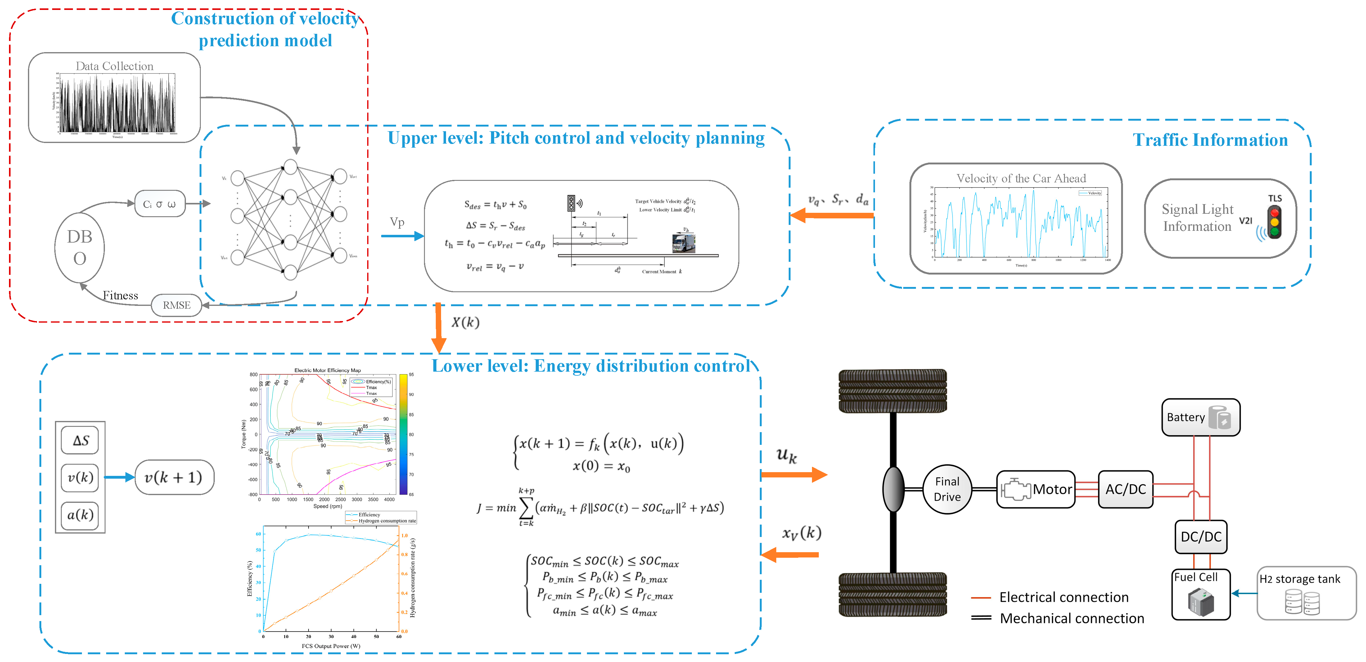
  • A hierarchical energy management strategy tailored for fuel cell commercial vehicles integrating traffic information is proposed. Based on the large framework of MPC, a hierarchical energy management strategy is constructed. In the upper layer, an optimal economic velocity for the vehicle is planned by considering the front vehicle velocity, the following distance, and the traffic light information. The lower layer allocates the power of each power source in accordance with the sequence of the optimal economic velocity.
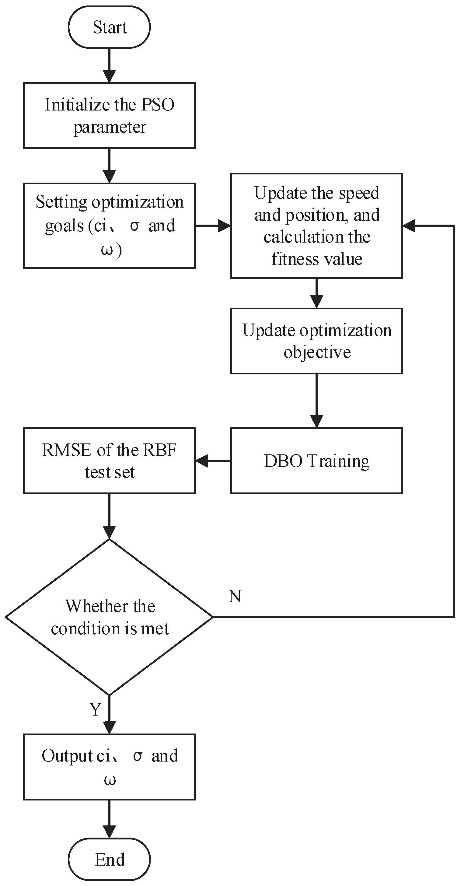
  • The dung beetle optimization-radial basis function (DBO-RBF) neural network prediction model is constructed. The performance of the model predictive control is closely related to the prediction accuracy. Therefore, the dung beetle optimization (DBO) algorithm is used to optimize the radial basis function (RBF) neural network, which improves both the velocity prediction accuracy and the operational velocity of the prediction model.
  • Different from the traditional velocity prediction, this paper predicts the future velocity of the front vehicle. The historical velocity information and environmental information of the preceding vehicle are used to predict the future velocity of the preceding vehicle.
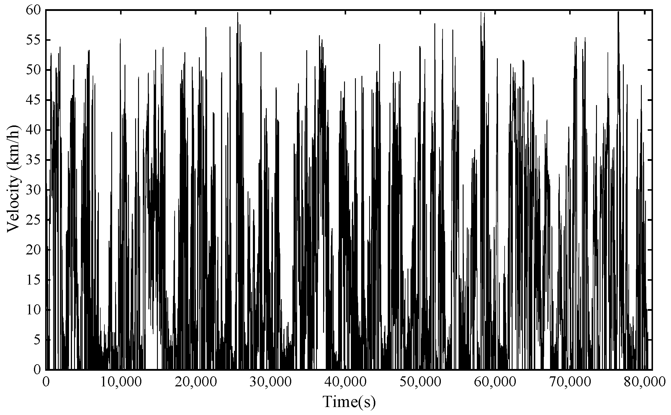
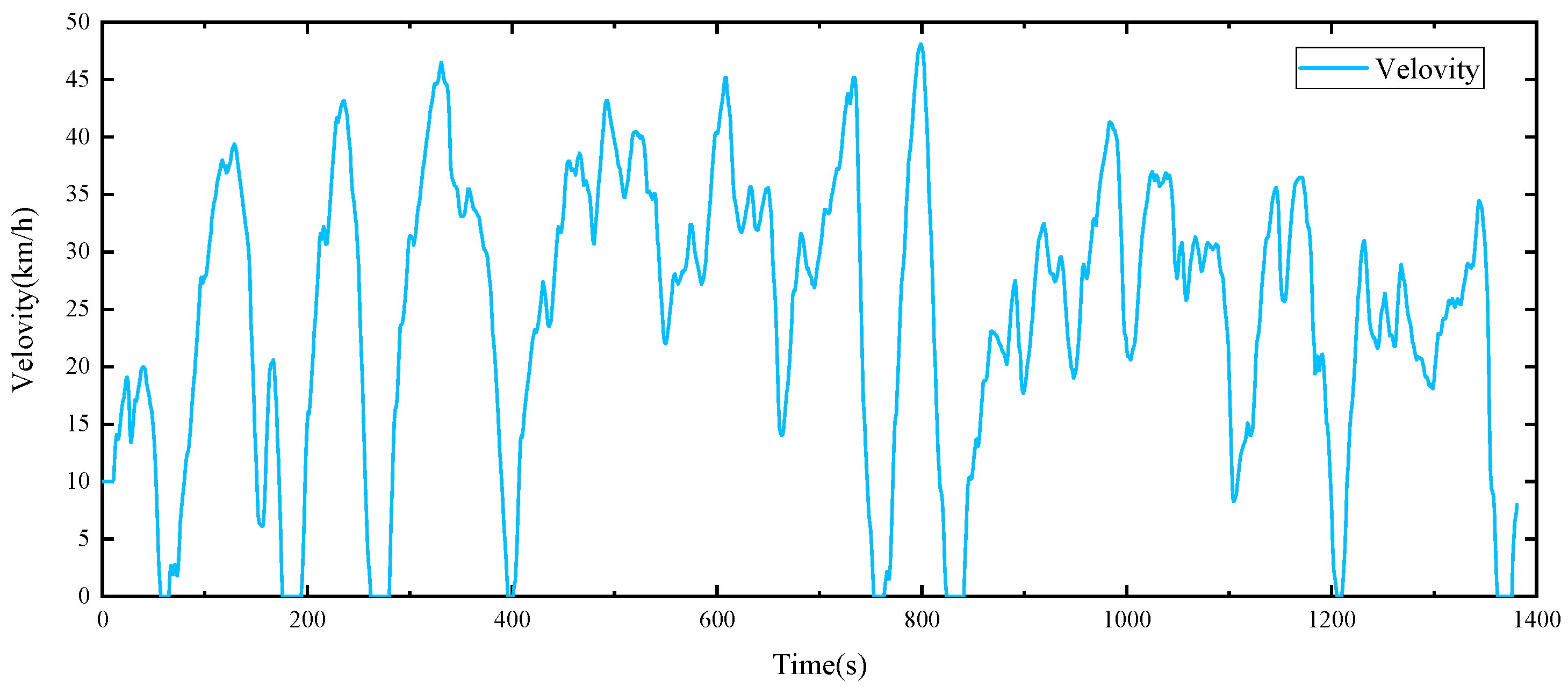
  • Real fuel cell commercial vehicle driving data are collected as the neural network training set is used. To make the simulation closer to the actual situation and avoid the limitations of the working conditions used in the training model, the velocity data of the real fuel cell commercial vehicle are collected, data processing is performed on these original data, and the processed data are used for training and testing.
The rest of this paper is arranged as follows: Section 2 introduces the fuel cell hybrid vehicle configuration and constructs the complete vehicle model; Section 3 describes the methodology of this study; Section 4 performs simulations and analyzes and discusses the simulation results; and Section 5 draws conclusions.

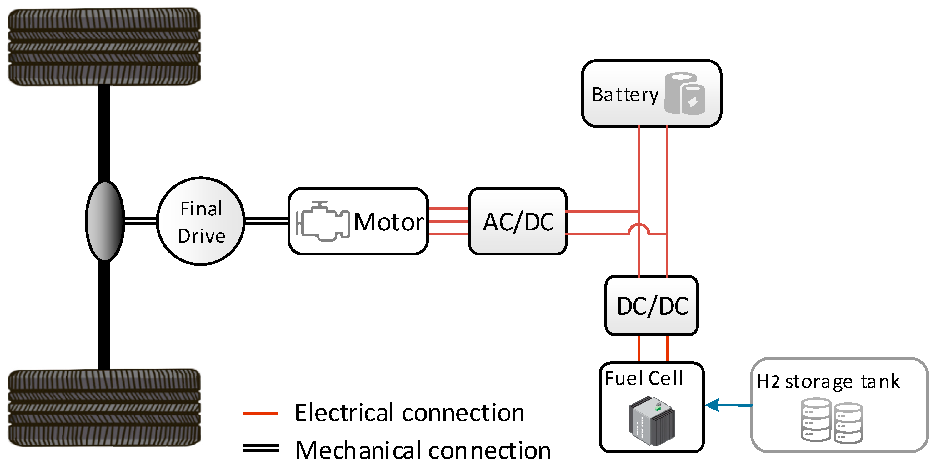
2. Vehicle System Configuration and Modeling

The subject of investigation in this scholarly article centers around a fuel cell hybrid commercial vehicle, with the vehicle’s configuration being depicted in Figure 1. Within the diagram, the black line signifies the mechanical connection, the red line represents the electrical connection, and the blue line symbolizes the hydrogen flow channel. The hybrid power system of the vehicle comprises a fuel cell stack as the primary energy source and a power battery as the supplementary energy source. As the fuel cell stack is unable to recover energy, the power battery recovers and stores the braking energy during braking maneuvers. To ensure a stable bus voltage, the power battery is directly linked to the power bus, while the fuel cell is connected to the bus through a DC-DC converter. The pivotal parameters of the vehicle are shown in Table 1.

2.1. Vehicle Dynamics
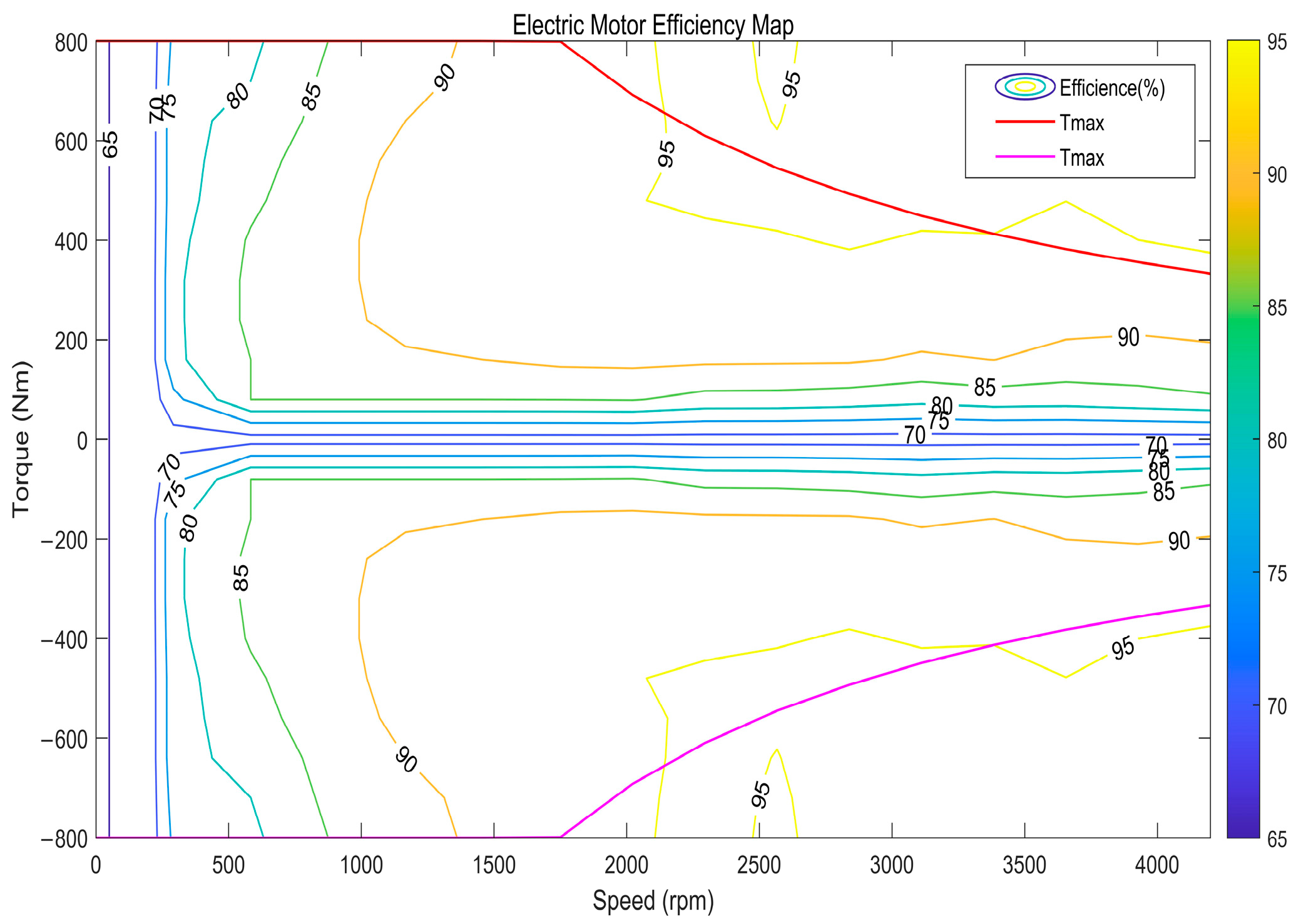
Ignoring the lateral dynamics of the vehicle, the driving resistance is an amalgamation of rolling resistance, air resistance, grade resistance, and acceleration resistance. Thus, the driving force equation of the vehicle is as follows:
                                              F t = m g f cos α + 1 2 ρ C d A v 2 + m g sin α + δ m d v d t
where m ,   g ,   f , and α represent the vehicle mass, gravity acceleration, rolling resistance coefficient, and road slope angle, respectively; ρ denotes air density; C d stands for the air resistance coefficient; A corresponds to the vehicle’s windward area; v signifies the vehicle velocity; δ is the conversion coefficient of rotating mass; and d v / d t refers to the vehicle acceleration.
The vehicle power requirements are
                                          P d = v η m g f cos α + 1 2 ρ C d A v 2 + m g sin α + δ m d v d t
where η is the drive train efficiency.

2.2. Motor Modeling

From Equation (1), the wheel speed and torque during vehicle driving can be further obtained, that is
ω w = v r
T w = r F t
where ω w ,   T w ,   r are the wheel speed, wheel torque, and wheel rolling radius, respectively. From this, the torque and power of the motor can be calculated using Equations (5) and (6).
T m = T w η i   T w 0 T w η i   T w < 0  
  P m = T m ω m η m   T m 0 T m ω m η m   T m < 0  
where T m and P m represent the torque and power of the motor, respectively, and η m denotes the efficiency of the motor. Neglecting other energy losses of the motor, the motor efficiency can be expressed as
η m = f n m ,   T m
The relevant parameters of the motor can be obtained by calculations and the parameters of the motor can be determined by matching. The map of the motor is shown in Figure 2.

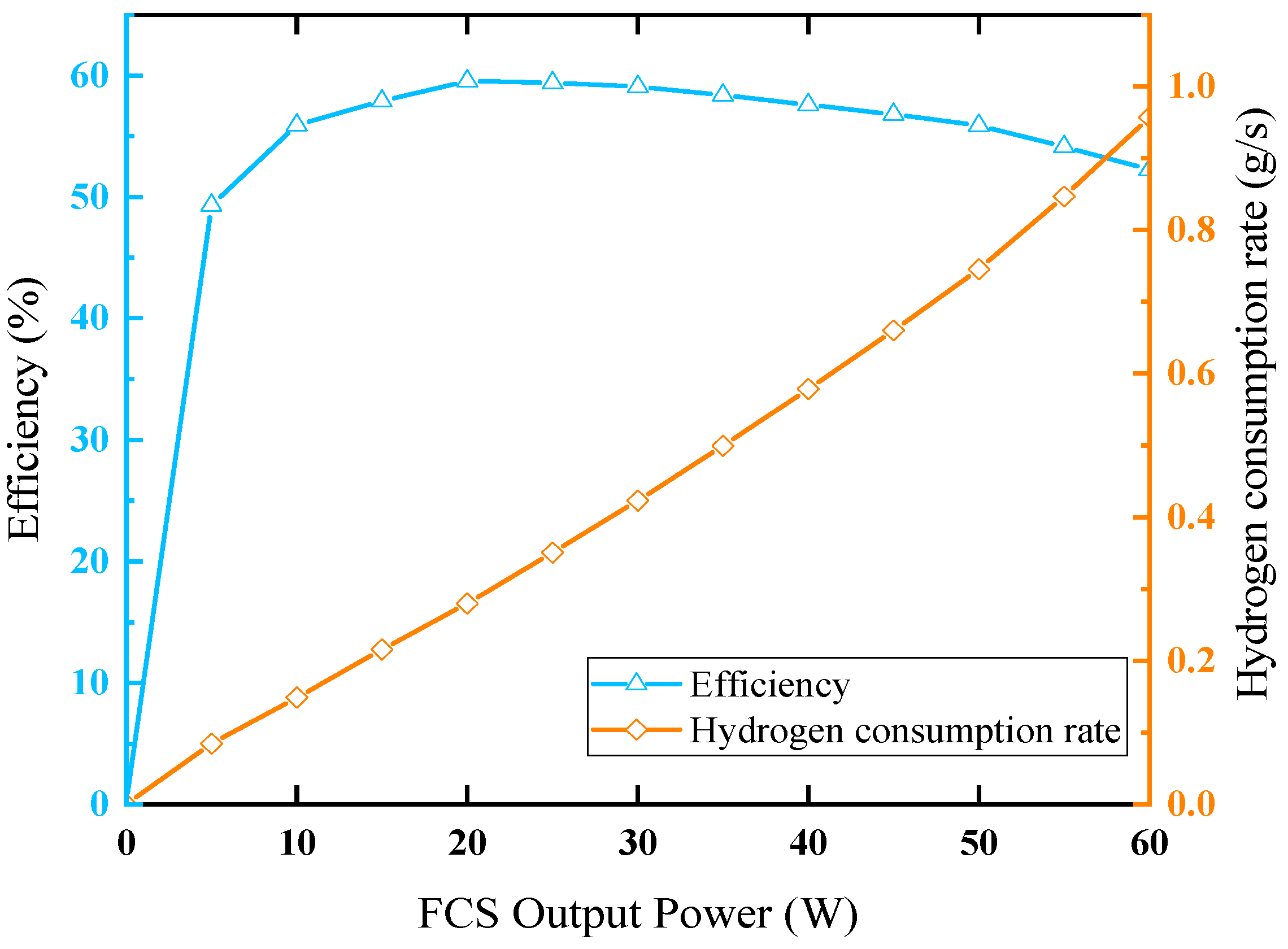
2.3. Fuel Cell System Modeling

The on-board fuel cell system comprises various components, including an air compressor, fuel cell stack, hydrogen storage system, hydrogen supply circuit, water circuit, and cooling system. Since this study solely focuses on the economy of the fuel cell system, a comprehensive system model is unnecessary. To accurately reflect the economy and enhance the model’s response speed, this paper constructs a fuel cell model using empirical and mathematical approaches [31,32]. It briefly describes the relationship between hydrogen consumption and output power. The fuel cell power can be determined by calculating the dynamic index of the vehicle. In this study, the rated power of the fuel cell is determined to be 60 kW through calculation. The fuel cell system is modeled as a single fuel cell linked in series. Three losses happen when a fuel cell is operating: the ohmic loss E o h i m i c , the activation loss E a c t , and the concentration difference loss E c o n . Consequently, the output voltage of the single fuel cell is
V c e l l = E n e r n s t E o h i m i c E a c t E c o n
The hydrogen consumption and output power of the fuel cell stack can be described as Equation (9).
P f c = N V c e l l I
m ˙ H 2 = N M H 2 n F I
where P f c represents the output power of the fuel cell system, N denotes the number of monomer fuel cells, F is the Faraday constant, M H 2 signifies the molar mass of hydrogen, and n represents the number of electrons lost during the electrochemical reaction. From this, the efficiency of the fuel cell can be derived as
η f c = P f c L H V m ˙ H 2
where L H V is the calorific value. The relationship between the output power and hydrogen consumption of the constructed fuel cell model is shown in Figure 3, and some parameters of the fuel cell are shown in Table 2.

2.4. Battery Modeling

The battery pack in this study can be described as an internal resistance model. The whole battery pack is connected with 87 single cells in series and 5 packs in parallel. The cell SOC, cell current I b , DC bus voltage U d c , and cell charging and discharging efficiency η c h g ,   η d i s can be calculated with Equations (12)–(15).
  S O C t = S O C 0 0 t η d i s I b t Q   I 0 S O C 0 0 t η c h g I b t Q   I < 0  
  I b = U o c S O C U o c S O C 2 4 P b t R b S O C 2 R b S O C
U d c = U o c S O C I b R b S O C
  η d i s = U o c S O C I b R d i s S O C U o c S O C = P b t U o c S O C I b η c h g = U o c S O C U o c S O C I b R c h g S O C = U o c S O C I b P b t  
where   Q   is the battery capacity and R b   represents the equivalent internal resistance.

3. Formulation of Control Strategy

The present section unveils the development of the layered strategy. This paper crafts a hierarchical energy management strategy, integrating traffic information, based on the MPC framework. The strategy amalgamates data from the motion state of the front vehicle and the traffic environment. Figure 4 illustrates the comprehensive structure of the hierarchical EMS. The MPC algorithm boasts four fundamental attributes: a predictive model, reference trajectory, rolling optimization, and feedback correction [33]. In essence, the MPC algorithm comprises three pivotal modules: the velocity prediction module, the solution algorithm module, and the control rule selection module [34]. During each prediction cycle, the velocity prediction module is used to predict the future vehicle velocity sequence utilizing historical and environmental information. Subsequently, the solution algorithm module determines the optimal control rules for the current prediction range. Lastly, the control rule selection module executes the application of the first element of the control sequence to the vehicle. At the next sampling time, the MPC controller repeats the above three processes until the entire drive cycle is completed [35]. The hierarchical energy management strategy proposed in this paper adopts an optimized RBF neural network as the prediction model and the upper and lower layers are effectively solved by the rolling optimization algorithm, founded on dynamic programming (DP).

3.1. Road Model

In order to avoid the limitations of the working conditions used in the training model, the actual driving data of the fuel cell commercial vehicles collected in this paper are used as the dataset. Due to the distortion of the actual collected data, it is necessary to process the original data. Firstly, the distorted fragments are removed, and then the remaining data are processed by wavelet filtering. The processed data are shown in Figure 5.
Then, a section of the road was selected as the final test condition, and the velocity of the selected section is shown in Figure 6. This section of the road, with a total length of about 9.5 km, passes 10 traffic lights. The signal timing and location information of this section of the road was recorded, as shown in Table 3. The initial state of the signal light model in this paper is set to green light and then converted to red light.

3.2. Improvement of The Prediction Model

In this section, we focus on designing the prediction module of MPC. Given that the effectiveness of MPC heavily relies on accurate predictions of state variables, including future velocity and vehicle power, we strived to enhance the precision of the RBF neural network. To achieve this, we employed the dung beetle optimization algorithm for optimizing the RBF neural network, thus creating the DBO-RBF neural network prediction model.
The RBF neural network, a forward neural network with a three-layer forward structure, was chosen for its simplicity, high prediction accuracy, and swift training speed. In this study, the Gaussian function is opted for as the basis function, and it is expressed as shown in Equation (16).
α x = e x p x c i 2 σ t 2
Then, the activation function of the neural network with the Gaussian kernel as the radial basis function is
R x , c i = e x p x c i 2 2 σ t 2
where x represents the input vector, c i represents the center of the Gaussian function, and σ signifies the variance of the Gaussian function, i.e., the radial basis width.
Therefore, the RBF neural network with Gaussian function as the basis function can be expressed as
Y x = i = 1 k ω i R x , c i
where Y x represents the output vector, k is the number of hidden layer neurons, and ω i signifies the connection weights of the RBF neural network.
The root mean square error (RMSE) was used as the evaluation index, and the calculation formula is shown in Equations (19) and (20).
R M S E k = k = 1 t p v k + i v 0 k + i 2 t p
R M S E = k = 1 n R M S E k n
where n denotes the number of sampling points, R M S E k represents the root mean square error in the prediction time domain of the kth sampling point, and t p signifies the length of prediction time. The center of the RBF neural network basis function c i , the width of the radial basis   σ , and the connection weight ω i between the hidden layer directly influence the output results of the radial basis neural network. As a result, an optimization algorithm was employed to optimize these three parameters, enhancing the prediction accuracy.
The dung beetle optimizer (DBO) [36], an algorithm inspired by the biological behavior of dung beetles, stands distinguished for its remarkable aptitude at seeking merits and swift convergence. Elaborate theoretical insights into the DBO can be gleaned from the referenced article [36]. The calculation process of the DBO algorithm chiefly encompasses the following steps:
(1) Commencing with the initialization of the parameters for the DBO algorithm;
(2) Proceeding to calculate the fitness values for all objectives, based on the objective function;
(3) Updating the location of all dung beetles;
(4) Verifying whether each target lies within the bounds;
(5) Updating the current optimal solution and its fitness value.
Throughout the program’s execution, the aforementioned steps are iterated until the termination criterion is fulfilled, ultimately resulting in the output of the global optimal solution and its corresponding fitness value.
During the rolling process, the position of the ball-rolling dung beetle is updated and can be expressed as
x i t + 1 = x i t + α × k × x i t 1 + b × x
x = x i t X w
where t represents the current iteration number, x i t denotes the position information of the ith dung beetle at the tth iteration, k 0 , 0.2 denotes a constant value which indicates the defection coefficient, b indicates a constant value belonging to (0, 1), α is a natural coefficient which is assigned as −1 or 1, X w indicates the global worst position, and x is used to simulate changes in light intensity.
The optimization parameters of the DBO algorithm are set as the center of the basis function, the width of the basis function, and the connection weight of the RBF neural network. The relationship can be expressed as
x i t = c i ,   σ ,   ω i
The fitness function is set to the RMSE of the training and test sets of the RBF neural network with the following expressions:
  f i n t e n e s s = R M S E p r e d i c t t r a i n + R M S E p r e d i c t t e s t
The flowchart of the constructed DBO-RBF algorithm is shown in Figure 7. The population size of DBO is 50, and the maximum number of iterations is 500.

3.3. Following Distance and Velocity Planning Model

The following distance was evaluated by the equivalent time headway method. The equivalent time headway refers to the time interval between the head of the vehicle and the front vehicle passing through a certain cross-section. The variable time headway (VTH) algorithm was used to control the spacing, and the future movement trend of the front vehicle was taken into account in the VTH algorithm. Through the prediction model in the previous section, the future motion state of the preceding vehicle can be predicted, and then the following distance and velocity can be adjusted by the VTH algorithm considering the movement trend of the preceding vehicle according to the predicted velocity sequence of the preceding vehicle so that the target vehicle can adjust the working condition in advance and improve the traffic efficiency of the vehicle.
The space between the two vehicles can be expressed as
S d e s = t h v + S 0
S = S r S d e s
where S d e s is the desired workshop distance, t h is the time headway, S 0 is the minimum safe vehicle distance, and v is the current velocity of this vehicle; S r is the actual two-vehicle spacing; and S is the error between the actual two-vehicle spacing and the desired workshop distance.
Among these components, the time headway t h can be expressed as
t h = t 0 c v v r e l c a a p
v r e l = v q v
where t 0 is the initial time headway; c v is the correlation coefficient greater than zero; c a is a constant greater than zero; a p is the acceleration of the front vehicle at the future moment, which can be calculated by the predicted front vehicle velocity above; and v q is the front vehicle velocity at the current moment. Considering the practical situation, the workshop time distance cannot be too large or too small, so the time headway is limited to
t hmin t h t hmax
To avoid the frequent acceleration and deceleration of the vehicle or excessive acceleration and deceleration velocities that affect driving comfort, the acceleration and the acceleration rate of change of the vehicle are controlled. The acceleration a and the rate of change of acceleration a of the vehicle can be calculated using the equations shown below:
a k = v k v k 1 / t s
a k = a k a k 1 / t s
The workshop distance error S , acceleration a , acceleration rate of change a , and the velocity of this vehicle are used as upper control system state variables, i.e.,
  X k = S k ; a k ; a k ; v k
The control variable is acceleration, and the acceleration formula of the vehicle is shown in Equation (33).
  a = T r e q / R w m g f cos α + 1 2 ρ C d A v 2 + m g sin α / m
The relevant parameters were set as follows: minimum safety distance S 0 = 7   m ; initial time headway t 0 = 1.5   s ; c v = 0.08 ; c a = 0.18 ; maximum time headway t hmin = 2   s ; minimum time headway t hmax = 0.4   s ; 3 a k 3 ; and 3 a k 3 .

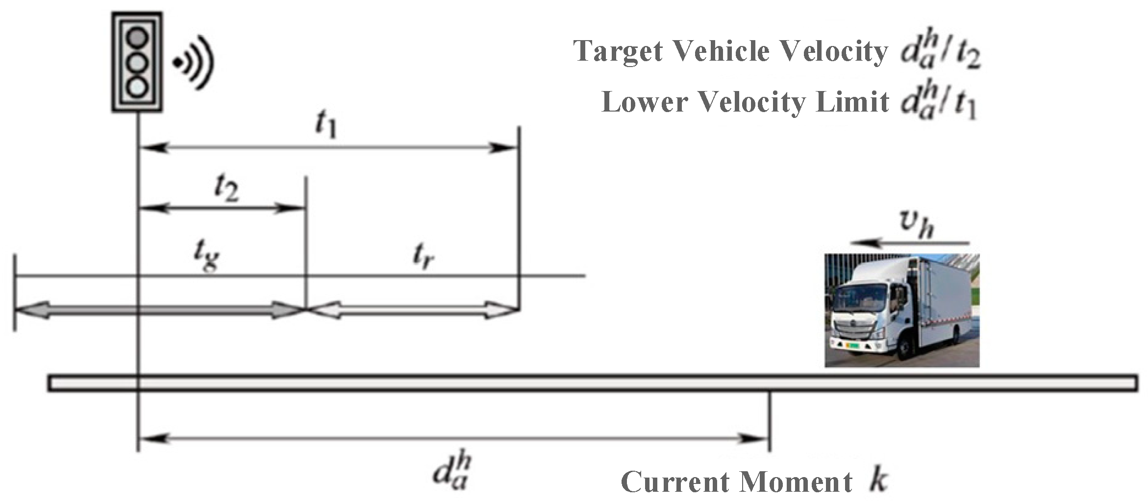
3.4. Vehicle Velocity Planning Model at Traffic Light Intersections

Based on the vehicle’s V2I technology, the vehicle can obtain information related to the traffic signal. Based on the acquired information about the distance between the vehicle and the traffic light and the timing of the traffic light, the economic velocity of the vehicle through the intersection can be planned. The velocity planning principle is shown in Figure 8.
In order to make the vehicle avoid parking through the intersection of traffic lights, there are two situations: when the next intersection is green and the maximum velocity of the vehicle meets the requirement to pass the intersection in the green light, the vehicle accelerates to the maximum velocity allowed to ensure that the vehicle passes the intersection before the red light. When the next intersection is red, the car must slow down early to ensure that it passes the intersection before the next green light. Therefore, there is an upper and lower velocity limit for passing through a red light intersection. The upper limit of the target velocity is calculated as follows:
v t a r h k = d a k T t c y c l e k The current light is red   v m a x The current light is green and   d a k T t c y c l e k t R v m a x d a k T t c y c l e k Other situations when the current light is green
light = Red   Light   0 mod k t c y c l e t R   Green   Light   t R mod k t c y c l e t c y c l e
t c y c l e = t R + t G
T k t c y c l e
v m a x = m i n v R ,   v p
where k is the current moment; v t a r h is the upper limit of the target velocity; d a is the distance between the vehicle and the traffic light; t R is the red light duration; and t G is the green light duration. To simplify the calculation, the yellow light time is included in t R ; t c y c l e is the cycle time of a signal; mod · is the residual function; T describes the number of traffic light cycles, and when k = t c y c l e , T increases by 1; v R is the velocity limit of the road; and v p is the velocity of the target vehicle at the next moment predicted by the velocity prediction model constructed in Section 3.2.
The lower limit of the target vehicle velocity, v t a r l , can be derived from Equation (39).
v t a r l k = d a k T t c y c l e k + t G The current light is red d a k T t c y c l e k t R The current light is green and   d a k T t c y c l e k t R v m a x d a k T t c y c l e k + t G Other situations when the current light is green

3.5. DP-Based MPC solver

The dynamic programming algorithm can obtain the global optimal solution, while the MPC strategy needs to solve the constraint problem in the finite time domain. Therefore, the dynamic programming algorithm combined with MPC can transform global optimization into local optimization, avoiding the need to obtain global working conditions. At the same time, MPC has the characteristics of rolling optimization, which can avoid falling into local optimization.
For the lower-level energy management strategy, the SOC and power distribution factor need to be used as state variables and control variables. In addition, it is also necessary to solve the control variables in the upper level velocity planning module described in Section 3.3. Considered comprehensively, the SOC, power distribution factor, workshop distance error S , acceleration a , acceleration change rate a , and vehicle velocity are used as state variables; the SOC, power distribution factor, and acceleration a are control variables. The state variables are discretized, as shown in Equation (40).
  x k + 1 = f k x k ,   u k   k = 0 ,   1 ,   2 ,   ,   N
where x k + 1 is the state variable at moment k + 1 ; f k is the state transfer equation; u k is the control variable; and N is the driving cycle length. The objective function is
  J = m i n t = k k + p α m ˙ H 2 + β S O C t S O C t a r 2 + γ S
The constraints are as follows:
  S O C m i n S O C k S O C m a x P b _ m i n P b k P b _ m a x P f c _ m i n P f c k P f c _ m a x a m i n a k a m a x
where S O C m i n is the minimum value of the SOC, which is taken as 0.3; S O C m a x is the maximum value of the SOC, which is taken as 0.8; P b _ m i n is the maximum charging power of the power cell; P b _ m a x is the maximum discharging power of the power cell; P f c _ m i n is the minimum power of the fuel cell; and P f c _ m a x is the maximum power of the fuel cell.

4. Validation and Discussion

The validation of the aforementioned model is the first step in this section, after which the effectiveness of the suggested hierarchical MPC is evaluated. A comparison is made against both the dynamic programming algorithm and the rule-based policy to thoroughly evaluate the efficacy of the proposed EMS. A simulation is performed on the assumption that the car travels on a level road with little variation in the road’s slope. On a laptop with an AMD Ryzen 7 4800H CPU operating at 2.9 GHz, the simulations were conducted using MATLAB 2020a.

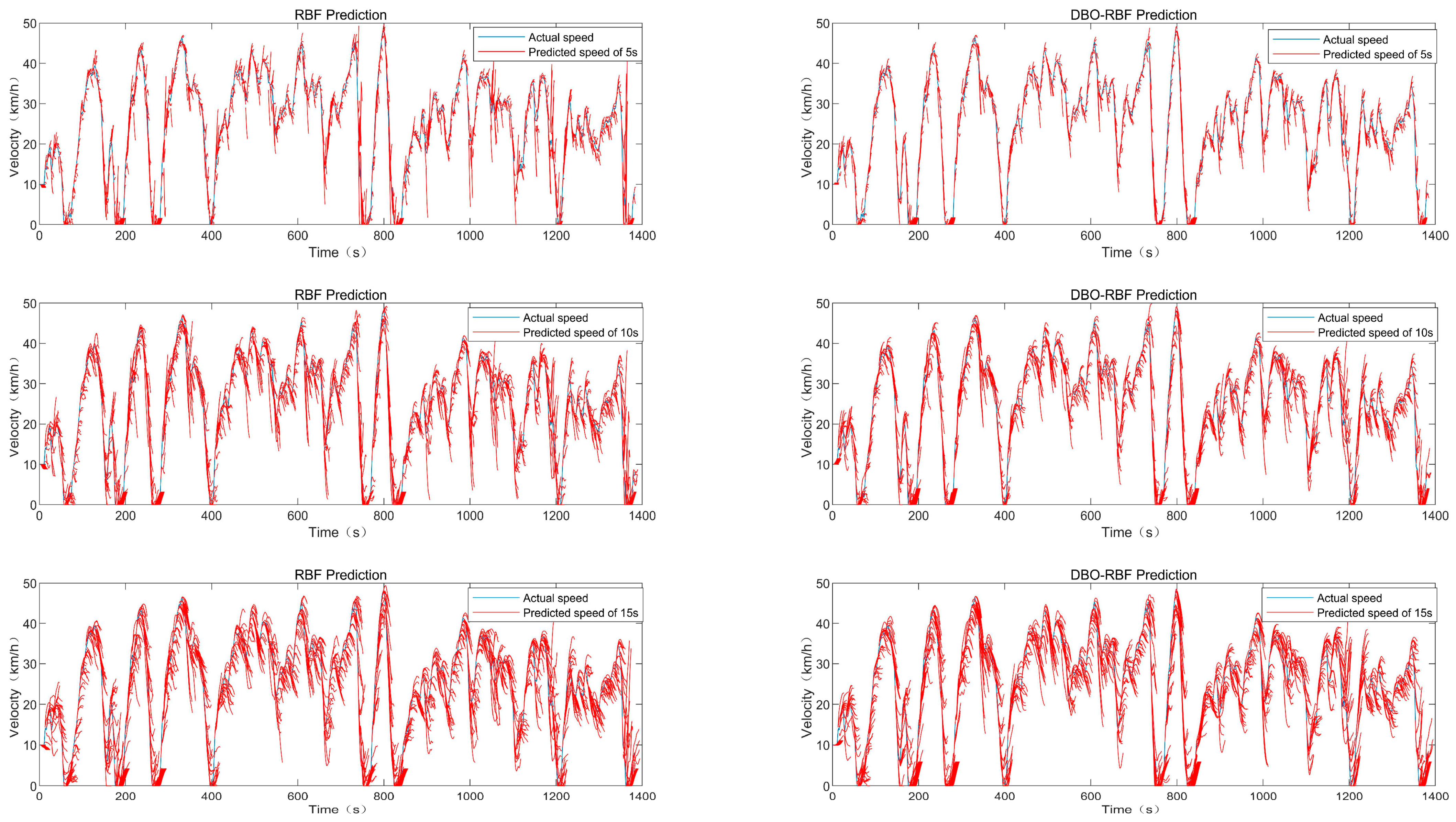
4.1. Optimization Effect of RBF Neural Network Prediction Model

This section will verify the performance of the DBO-RBF neural network prediction model constructed in Section 3.2. The neural network underwent training using the pre-processed dataset described in Section 3.1, where 80% served as the training set and 20% was designated as the test set. The trained velocity prediction model was then validated using the final test section. It is noteworthy that the length of the prediction range significantly impacts the prediction model’s performance. Thus, this paper analyzes various prediction ranges. The historical velocity range collected by the prediction model was set to 10 s, and the prediction ranges of 5 s, 10 s, and 15 s were tested. The velocity prediction effects of different prediction ranges before and after optimization are shown in Figure 9, and Table 4 shows the RMSE of the prediction effects before and after optimization.
From the simulation data in Figure 9 and Table 4, it can be seen that the optimized prediction model has a significant improvement in prediction accuracy. It can be seen that the larger the prediction range is, the worse the prediction accuracy is and the less obvious the optimization effect is, and the most obvious improvement effect is at the prediction length of 5 s. In addition, setting the prediction length to 5 s can also improve the operation velocity of the prediction model, so the prediction length was set to 5 s.

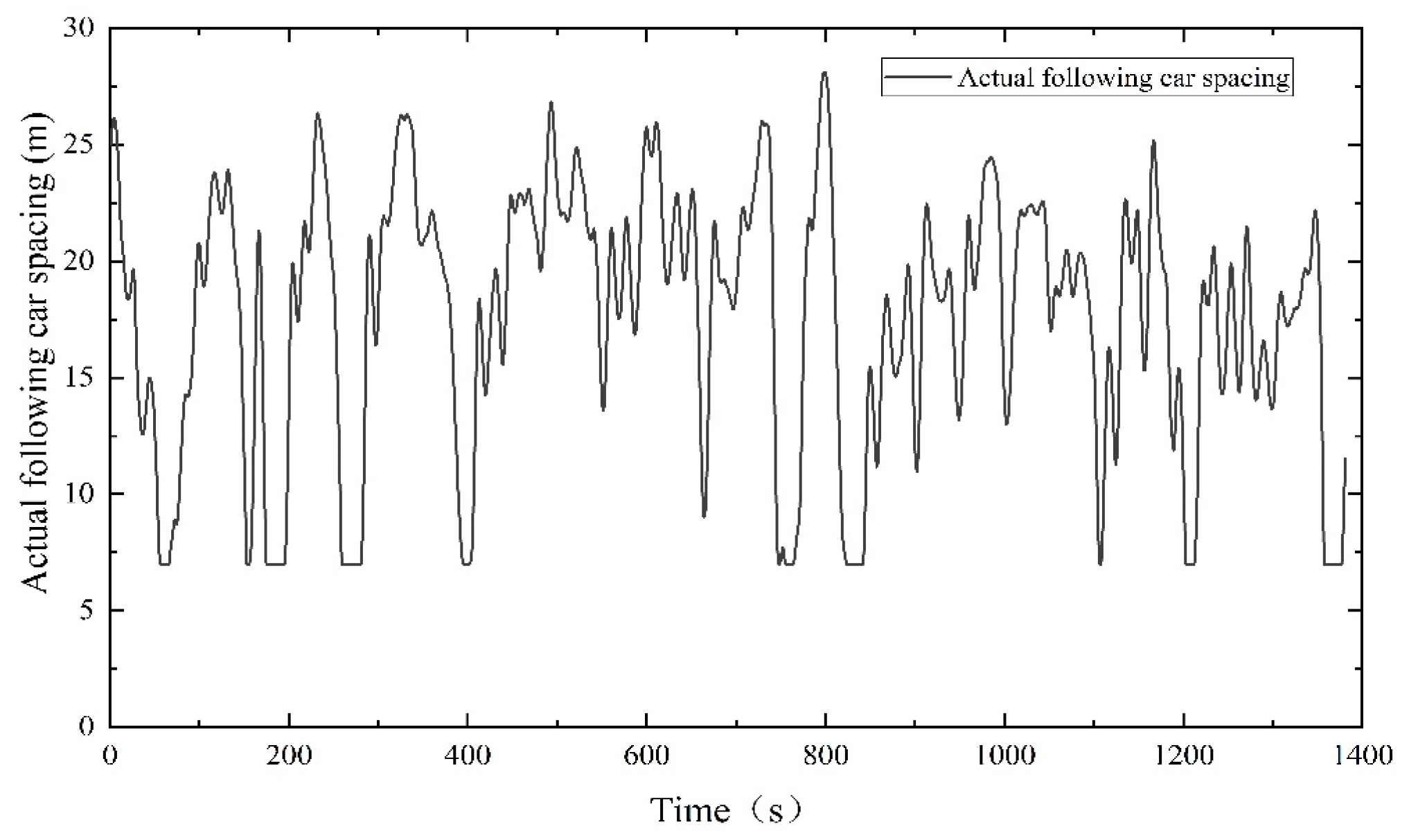
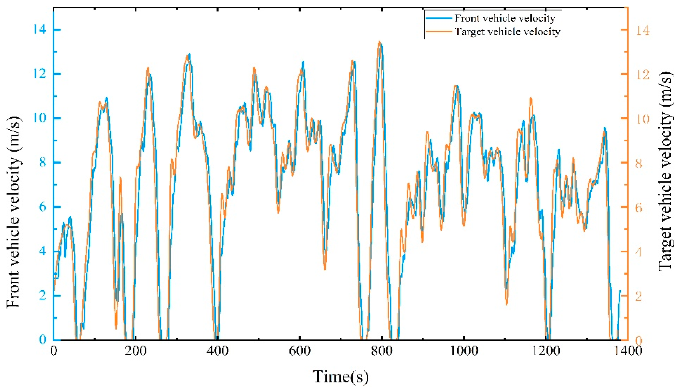
4.2. Verification of the Effect of the Upper Layer Spacing and Velocity Planning Model

Using the final test conditions described in Section 3.1, the upper level following distance and velocity planning model described in Section 3.3 was simulated. The simulation results are shown in Figure 10 and Figure 11.
From Figure 10 and Figure 11, it can be seen that the target vehicle can follow the front vehicle well, and the vehicle keeps a large following distance when the velocity is high to avoid causing safety problems; it keeps a smaller distance when the velocity is low to improve the road utilization, which is in line with the design expectation. In addition, since the prediction model is used to predict the motion state of the front vehicle, the target vehicle can respond to the front road condition in advance according to the prediction results.

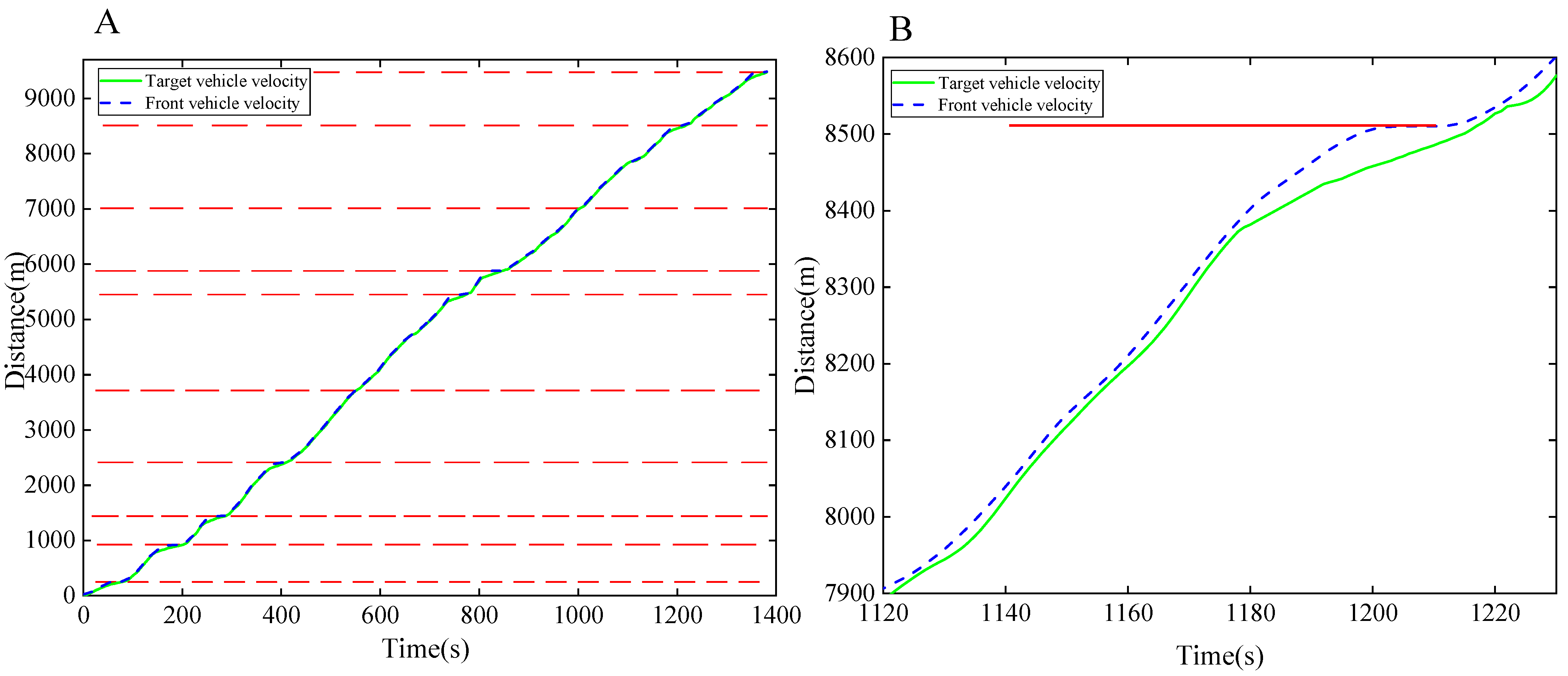
4.3. Verification of Velocity Planning Model at Traffic Light Intersection

Using the road model brought to the final test condition, the velocity planning model at the traffic light intersection constructed in Section 3.4 was simulated and validated, and the simulation results are shown in Figure 12.
In Figure 12, Figure 12A shows the effect of the whole working condition, and Figure 12B is the local zoomed-in figure of the vehicle passing the ninth traffic light intersection. The red line segment in the figure indicates that the traffic light is in red; the blue dashed line in the figure is the travel distance curve of the vehicle ahead, while the green solid line is that of the target vehicle. It can be seen in Figure 12 that the model has a good control effect. Under the control of the model, the target vehicle travels at the velocity planned by the model constructed in Section 3.3 when it does not reach the traffic light intersection; when it reaches the traffic light intersection, the velocity planning model constructed for the traffic light intersection starts to take effect, and the vehicle will adjust its velocity in advance to avoid stopping at the traffic light intersection. At this time, the main goal is to avoid stopping at the traffic light intersection, so the distance between the two vehicles will increase; after passing the traffic light intersection, the target vehicle continues to drive according to the velocity planning of the model constructed in Section 3.3, and the distance between the two vehicles gradually decreases.

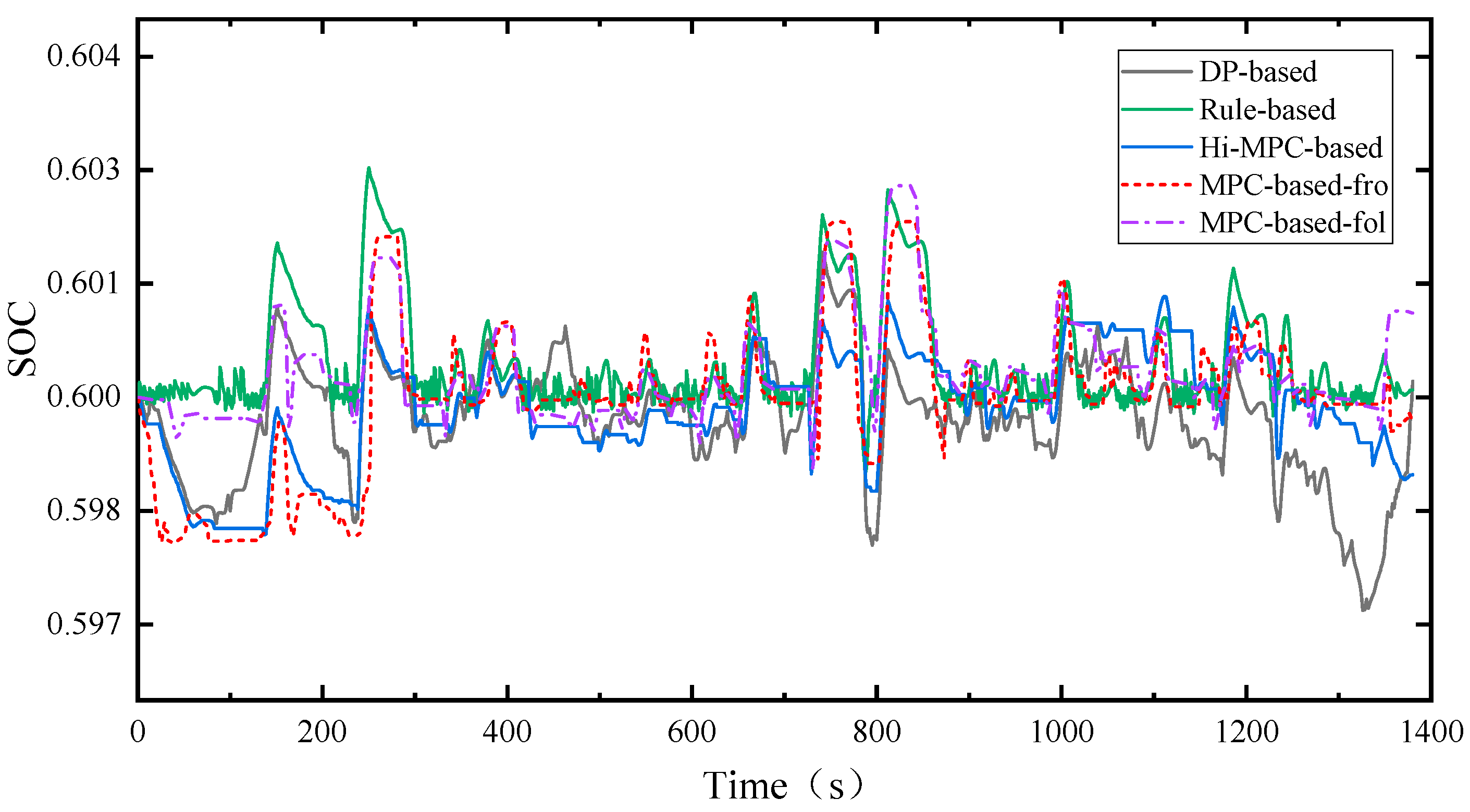
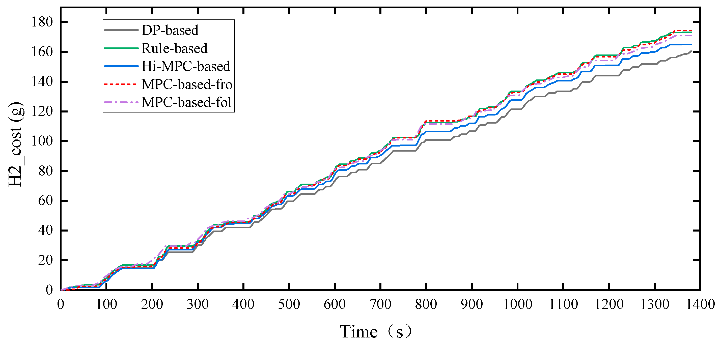
4.4. Overall Performance Verification of Hierarchical EMS

In this section, the overall performance of the proposed hierarchical EMS is verified based on the final test conditions described in Section 3.1. It is assumed that at the beginning when the two vehicles are driving in the same direction on the road with a 25 m distance between them, the target vehicle velocity is 8km/h and the front vehicle velocity is 10 km/h. After that, the front vehicle is driving according to the final test working condition and the target vehicle is controlled by the proposed strategy. In addition, dynamic planning-based and rule-based energy management strategies are constructed to compare with the proposed strategy to analyze the performance of the proposed strategy. In this paper, the initial SOC is set to 0.6 and the desired final value of the SOC is also set to 0.6. Based on the analysis in Section 4.1, the prediction length of the DBO-RBF neural network prediction model is set to 5 s.
Figure 13 shows the SOC curves of different strategies in different cases, where the black solid line represents the energy management strategy of the DP algorithm, the green solid line represents the rule-based energy management strategy, the blue solid line represents the proposed hierarchical energy management strategy, and the red dotted line represents the SOC curve when the hierarchical energy management strategy is applied to the vehicle in front, named MPC-based-fro represents, and MPC-based-fol with a purple dotted line represents the SOC curve of the hierarchical energy management strategy considering only the distance control between the followers. Table 5 shows the H2 consumption of these EMSs, and E-Cost represents the equivalent hydrogen consumption when equating the SOC to 0.6.
From Figure 13, it can be seen that regarding the changing trend of the SOC, the proposed hierarchical energy management strategy SOC change trend is consistent with the DP-based EMS, and because the acceleration change rate is taken into account, the Hi-MPC-based SOC change frequency is smaller and the relative change magnitude is not large. In addition, the SOC curve is smoother, which is beneficial to extend the battery life. From the statistical results in Table 5, it can be seen that the hydrogen consumption of the Hi-MPC-based strategy is the closest to that of the rule-based strategy under the comprehensive consideration of traffic information, and the equivalent hydrogen consumption is 96.4% after standardization compared to the rule-based approach. Compared with the rule-based strategy, the fuel economy is improved by about 3.97% under Hi-MPC-based control.
Since the car in front is traveling regularly, it may be said that the spacing control and information from the traffic lights are not taken into account. Therefore, MPC-based-fro and MPC-based-fol simulations were performed to consider the effect of the fusion of spacing control and traffic light information on the energy management strategy. Since both EMSs do not consider traffic light information, the vehicle decelerates and stops when passing through a traffic light intersection, so it can be seen that the SOC rises and flattens briefly around 300 s, 800 s, and 1200 s. The Hi-MPC-based strategy integrates spacing control and traffic light information, while MPC-based-fro only considers the following vehicles. The comparison of the two can show the effect of the fusion of traffic light information on the EMS. As can be seen from the statistics of the results in Table 5, the Hi-MPC-based strategy has a 1.81% improvement in fuel economy relative to MPC-based-fol, which shows that the fusion of traffic light information has an improvement effect on fuel economy. MPC-based-fro can be seen as neither considering the following spacing control nor considering the stoplight information or the traffic light information. The comparison with MPC-based-fro shows the effect of the following distance control on the EMS. The results in Table 5 show that the fuel economy of MPC-based-fol is 3.10% higher than that of MPC-based-fro, which shows that the following distance control has a certain influence on the EMS. The Hi-MPC-based strategy has 4.87% higher fuel economy than MPC-based-fro, which shows that the integrated consideration of traffic information has a better effect on the EMS than the fusion of one piece of information alone.
Figure 14 shows the hydrogen consumption curves of different strategies under different situations. It can be seen that the DP-based strategy is the optimal state of the vehicle with the highest economy under the comprehensive consideration of traffic information, while the rule-based strategy has the highest hydrogen consumption, and the proposed hierarchical strategy is in between and closest to the rule-based strategy. In addition, the integration of spacing control and traffic light information both result in some reduction in hydrogen consumption.

5. Conclusions

This paper introduces a novel hierarchical MPC fuel cell hybrid commercial vehicle energy management strategy, incorporating traffic information. Within this hierarchical EMS, the upper layer utilizes traffic data to design a more sensible vehicle driving velocity. Simultaneously, the lower layer employs a DP-algorithm-based solver to dynamically optimize vehicle power allocation, relying on the vehicle velocity sequence premeditated in the upper layer. Since the speed planning of the upper strategy is based on the prediction of the motion state of the front vehicle, in order to improve the accuracy of the speed planning of the upper strategy, this paper first constructs a DBO-RBF neural network prediction model, which is used to predict the motion state of the front vehicle. The DBO algorithm is used to optimize the parameters of the RBF neural network. When the prediction length is 5 s, the accuracy is improved by 13.96%, which significantly improves the prediction accuracy. Then, when passing through a traffic light intersection, the traffic light information is also considered in the speed planning of the upper layer strategy, which comprehensively considers the motion state of the vehicle in front and the traffic light information to plan a more economical vehicle travel speed to improve the traffic efficiency of the vehicle and the road utilization rate. Finally, the overall performance of the proposed strategy is meticulously assessed. The results affirm that the fuel economy of the proposed strategy exceeds the traditional rule-based strategy by 3.97%. In addition, the integration of traffic information imparts a definite fuel economy boost of 4.87% as compared to scenarios not considering such data. By skillfully incorporating traffic information, the proposed strategy bolsters vehicle traffic efficiency, enhances road utilization, and simultaneously upholds the fuel economy and power performance of the vehicles.
In future research, the vehicle spacing control of fused traffic information can be further researched. In this paper, we only consider the case of following a vehicle, and we do not consider the case of a vehicle turning in front of us or other vehicles merging into the lane. Speed planning methods with multi-signal information can also be considered. In this study, the vehicle velocity is planned according to the next traffic light state, while in real life, the commercial vehicle driving section is more fixed. With the development of technology, the traffic light information of the whole road section can be obtained in the future, and a more economical velocity can be obtained by planning the velocity according to multiple traffic light information. In addition, in this paper, only the effect under urban conditions is investigated, and in future studies, the situation under other conditions or at higher speeds can be further investigated.

Author Contributions

Conceptualization, Y.X., E.X. and W.Z.; methodology, Y.X. and W.Z.; software, W.Z. and Y.X.; validation, Y.X., E.X., W.Z. and Q.H.; investigation, Q.H.; data curation, E.X. and W.Z.; writing—original draft preparation, Y.X.; writing—review and editing, W.Z., E.X. and Q.H.; visualization, E.X. and Y.X.; project administration, W.Z. and E.X. All authors have read and agreed to the published version of the manuscript.

Funding

This research was funded by the Innovation-Driven Development Special Fund Project of Guangxi (Grant No. Guike AA22068060) and the Science and Technology Planning Project of Liuzhou (Grant No. 2022AAA0102, 2022AAA0104).

Institutional Review Board Statement

Not applicable.

Informed Consent Statement

Not applicable.

Data Availability Statement

Data are available on reasonable demand from the corresponding author.

Conflicts of Interest

The authors declare no conflict of interest.

References

  1. Ahmadi, P.; Torabi, S.H.; Afsaneh, H.; Sadegheih, Y.; Ganjehsarabi, H.; Ashjaee, M. The effects of driving patterns and PEM fuel cell degradation on the lifecycle assessment of hydrogen fuel cell vehicles. Int. J. Hydrog. Energy 2019, 45, 3595–3608. [Google Scholar] [CrossRef]
  2. Hames, Y.; Kaya, K.; Baltacioglu, E.; Turksoy, A. Analysis of the control strategies for fuel saving in the hydrogen fuel cell vehicles. Int. J. Hydrog. Energy 2018, 43, 10810–10821. [Google Scholar] [CrossRef]
  3. Fernandez, L.M.; Garcia, P.; Garcia, C.A.; Jurado, F. Hybrid electric system based on fuel cell and battery and integrating a single dc/dc converter for a tramway. Energy Convers. Manag. 2010, 52, 2183–2192. [Google Scholar] [CrossRef]
  4. Sulaiman, N.; Hannan, M.A.; Mohamed, A.; Ker, P.J.; Majlan, E.H.; Daud, W.R.W. Optimization of energy management system for fuel-cell hybrid electric vehicles: Issues and recommendations. Appl. Energy 2018, 228, 2061–2079. [Google Scholar] [CrossRef]
  5. IoanSorin, S.; Nicu, B.; Phatiphat, T.; Mihai, V.; Elena, C.; Mihai, C.; Mariana, I.; Mircea, R. Fuel Cell Electric Vehicles—A Brief Review of Current Topologies and Energy Management Strategies. Energies 2021, 14, 252. [Google Scholar] [CrossRef]
  6. Shaohua, L.; Changqing, D.; Fuwu, Y.; Jun, W. A rule-based energy management strategy for a new BSG hybrid electric vehicle. In Proceedings of the 2012 Third Global Congress on Intelligent Systems, Wuhan, China, 6–8 November 2012; pp. 209–212. [Google Scholar]
  7. Changqing, D.; Shiyang, H.; Yuyao, J.; Dongmei, W.; Yang, L. Optimization of Energy Management Strategy for Fuel Cell Hybrid Electric Vehicles Based on Dynamic Programming. Energies 2022, 15, 4325. [Google Scholar] [CrossRef]
  8. Veer, S.K.; Om, B.H.; Dheerendra, S. Fuzzy logic and Elman neural network tuned energy management strategies for a power-split HEVs. Energy 2021, 225, 120152. [Google Scholar] [CrossRef]
  9. Trinh, H.-A.; Truong, H.-V.-A.; Ahn, K.K. Development of fuzzy-adaptive control based energy management strategy for PEM fuel cell hybrid tramway system. Appl. Sci. 2022, 12, 3880. [Google Scholar] [CrossRef]
  10. Yanwei, L.; Jiansheng, L.; Jiaqing, S.; Ye, J. Research on Energy Management Strategy of Fuel Cell Vehicle Based on Multi-Dimensional Dynamic Programming. Energies 2022, 15, 5190. [Google Scholar] [CrossRef]
  11. Hujun, P.; Zhu, C.; Jianxiang, L.; Kai, D.; Steffen, D.; Jonas, G.; Cem, Ü.; Andreas, T.; Lars, L.; Stefan, P.; et al. Offline optimal energy management strategies considering high dynamics in batteries and constraints on fuel cell system power rate: From analytical derivation to validation on test bench. Appl. Energy 2021, 282, 116152. [Google Scholar] [CrossRef]
  12. Jiayi, H.; Jianqiu, L.; Zunyan, H.; Liangfei, X.; Ouyang, M. Power distribution strategy of a dual-engine system for heavy-duty hybrid electric vehicles using dynamic programming. Energy 2021, 215, 118851. [Google Scholar] [CrossRef]
  13. Paganelli, G.; Delprat, S.; Guerra, T.-M.; Rimaux, J.; Santin, J.-J. Equivalent consumption minimization strategy for parallel hybrid powertrains. In Proceedings of the Vehicular Technology Conference, IEEE 55th Vehicular Technology Conference, VTC Spring 2002 (Cat. No. 02CH37367), Birmingham, AL, USA, 6–9 May 2002; pp. 2076–2081. [Google Scholar]
  14. Yuanjian, Z.; Liang, C.; Zicheng, F.; Nan, X.; Chong, G.; Di, Z.; Yang, O.; Lei, X. Energy management strategy for plug-in hybrid electric vehicle integrated with vehicle-environment cooperation control. Energy 2020, 197, 117192. [Google Scholar] [CrossRef]
  15. Lin, X.; Zhou, K.; Li, H. AER adaptive control strategy via energy prediction for PHEV. IET Intell. Transp. Syst. 2019, 13, 1822–1831. [Google Scholar] [CrossRef]
  16. Srinivasan, S.; Tiwari, R.; Krishnamoorthy, M.; Lalitha, M.P.; Raj, K.K. Neural network based MPPT control with reconfigured quadratic boost converter for fuel cell application. Int. J. Hydrog. Energy 2021, 46, 6709–6719. [Google Scholar] [CrossRef]
  17. Pereira, D.F.; da Costa Lopes, F.; Watanabe, E.H. Nonlinear model predictive control for the energy management of fuel cell hybrid electric vehicles in real time. IEEE Trans. Ind. Electron. 2020, 68, 3213–3223. [Google Scholar] [CrossRef]
  18. Xinyou, L.; Zhaorui, W.; Jiayun, W. Energy management strategy based on velocity prediction using back propagation neural network for a plug-in fuel cell electric vehicle. Int. J. Energy Res. 2021, 45, 2629–2643. [Google Scholar] [CrossRef]
  19. Xuncheng, C.; Shengwei, Q.; Jinzhou, C.; Ya-Xiong, W.; He, H. Proton exchange membrane fuel cell-powered bidirectional DC motor control based on adaptive sliding-mode technique with neural network estimation. Int. J. Hydrog. Energy 2020, 45, 20282–20292. [Google Scholar] [CrossRef]
  20. Huachun, T.; Hailong, Z.; Jiankun, P.; Zhuxi, J.; Yuankai, W. Energy management of hybrid electric bus based on deep reinforcement learning in continuous state and action space. Energy Convers. Manag. 2019, 195, 548–560. [Google Scholar] [CrossRef]
  21. Xuechao, W.; Jinzhou, C.; Shengwei, Q.; Ya-Xiong, W.; Hongwen, H. Hierarchical model predictive control via deep learning vehicle speed predictions for oxygen stoichiometry regulation of fuel cells. Appl. Energy 2020, 276, 115460. [Google Scholar] [CrossRef]
  22. Darbha, S.; Konduri, S.; Pagilla, P.R. Benefits of V2V Communication for Autonomous and Connected Vehicles. IEEE Trans. Intell. Transp. Syst. 2019, 20, 1954–1963. [Google Scholar] [CrossRef]
  23. Hongbo, G.; Shengbo, L.; GuoTao, X. Discrete-time model predictive control for lateral trajectory tracking of Intelligent cars. J. Command. Control. 2018, 4, 297–305. [Google Scholar]
  24. Qiuyi, G.; Zhiguo, Z.; Peihong, S.; Peidong, Z. Optimization management of hybrid energy source of fuel cell truck based on model predictive control using traffic light information. Control. Theory Technol. 2019, 17, 309–324. [Google Scholar] [CrossRef]
  25. Kaijiang, Y.; Junqi, Y.; Daisuke, Y. Model predictive control for hybrid vehicle ecological driving using traffic signal and road slope information. Control. Theory Technol. 2015, 13, 17–28. [Google Scholar] [CrossRef]
  26. Fengqi, Z.; Junqiang, X.; Reza, L. Real-Time Energy Management Strategy Based on Velocity Forecasts Using V2V and V2I Communications. IEEE Trans. Intell. Transp. Syst. 2017, 18, 416–430. [Google Scholar] [CrossRef]
  27. Chenglin, L.; Jianqiang, W.; Wenjuan, C.; Yuzhao, Z. An Energy-Efficient Dynamic Route Optimization Algorithm for Connected and Automated Vehicles Using Velocity-Space-Time Networks. IEEE Access 2019, 7, 108866–108877. [Google Scholar] [CrossRef]
  28. Xiaolin, T.; Shanshan, L.; Hong, W.; Ziwen, D.; Yinong, L. Research on energy control strategy based on hierarchical model predictive control in connected environment. J. Mech. Eng. 2020, 56, 119–128. [Google Scholar] [CrossRef]
  29. Hongwen, H.; Yunlong, W.; Ruoyan, H.; Mo, H.; Yunfei, B.; Qingwu, L. An improved MPC-based energy management strategy for hybrid vehicles using V2V and V2I communications. Energy 2021, 225, 120273. [Google Scholar] [CrossRef]
  30. Fengqi, Z.; Xiaosong, H.; Teng, L.; Kanghui, X.; Ziwen, D.; Hui, P. Computationally Efficient Energy Management for Hybrid Electric Vehicles Using Model Predictive Control and Vehicle-to-Vehicle Communication. IEEE Trans. Veh. Technol. 2021, 70, 237–250. [Google Scholar] [CrossRef]
  31. Pukrushpan, J.T.; Peng, H.; Stefanopoulou, A.G. Control-Oriented Modeling and Analysis for Automotive Fuel Cell Systems. J. Dyn. Syst. Meas. Control. 2004, 126, 14–25. [Google Scholar] [CrossRef]
  32. Shan-Jen, C.; Jui-Jung, L. Nonlinear modeling and identification of proton exchange membrane fuel cell (PEMFC). Int. J. Hydrog. Energy 2015, 40, 9452–9461. [Google Scholar] [CrossRef]
  33. Morari, M.; Barić, M. Recent developments in the control of constrained hybrid systems. Comput. Chem. Eng. 2006, 30, 1619–1631. [Google Scholar] [CrossRef]
  34. Shuo, Z.; Rui, X.; Fengchun, S. Model predictive control for power management in a plug-in hybrid electric vehicle with a hybrid energy storage system. Appl. Energy 2017, 185, 1654–1662. [Google Scholar] [CrossRef]
  35. Weiwei, X.; Enyong, X.; Weiguang, Z.; Haibo, F.; Jirong, Q. Optimal energy management of fuel cell hybrid electric vehicle based on model predictive control and on-line mass estimation. Energy Rep. 2022, 8, 4964–4974. [Google Scholar] [CrossRef]
  36. Jiankai, X.; Bo, S. Dung beetle optimizer: A new meta-heuristic algorithm for global optimization. J. Supercomput. 2023, 79, 7305–7336. [Google Scholar] [CrossRef]
Figure 1. Configuration of fuel cell and battery hybrid propulsion system.
Sustainability 15 12833 g001
Figure 2. Electric motor efficiency map.
Sustainability 15 12833 g002
Figure 3. Efficiency and hydrogen consumption characteristic curves of FCS.
Sustainability 15 12833 g003
Figure 4. Hierarchical EMS structure.
Sustainability 15 12833 g004
Figure 5. Velocity data after pre-processing.
Sustainability 15 12833 g005
Figure 6. The final test set data.
Sustainability 15 12833 g006
Figure 7. Flowchart of the DBO-RBF algorithm.
Sustainability 15 12833 g007
Figure 8. Principle of traffic velocity planning at traffic light intersections.
Sustainability 15 12833 g008
Figure 9. Comparison of RBF and DBO-RBF with different prediction ranges.
Sustainability 15 12833 g009
Figure 10. Actual following vehicle spacing controlled by upper layer algorithm.
Sustainability 15 12833 g010
Figure 11. The velocity of the following vehicle planned by the upper layer algorithm.
Sustainability 15 12833 g011
Figure 12. Effect of velocity planning model at traffic light intersection: (A) shows the effect of the whole working condition; (B) is the local zoomed-in figure of the vehicle passing the 9th traffic light intersection. The red line segment in the figure indicates that the traffic light is in red.
Sustainability 15 12833 g012
Figure 13. SOC curves under different strategies.
Sustainability 15 12833 g013
Figure 14. H2 cost curves under different strategies.
Sustainability 15 12833 g014
Table 1. Parameter of the full cell hybrid vehicle.
ParameterValueUnit
Vehicle total mass6000kg
Wheel radius0.375m
Gravitational acceleration9.8m/s2
Air density6.125kg/m3
Aerodynamic drag coefficient0.492-
Final drive gear ratio6.5071-
Transmission efficiency95%
Table 2. Parameter of the PEMFC.
ParameterSymbolValue
Number of cells in the stackN300
Full cell active areaA280 cm2
Thickness of the membrane layerL50 μm
Universal gas constantR 8.314   J / ( mol · k)
Faraday’s constantF96,485.34 C/mol
Table 3. Signal timing and location information.
Signal Lamp Number12345678910
Green light duration (s)25281830253325354036
Red light duration (s)40695270667680657050
Cycle duration (s)6597701009110910510011086
Distance from the starting point (m)22389714132388368954255855703784869452
Table 4. Comparison of RMSE of RBF and DBO-RBF.
RMSEPrediction Lengths
5 s10 s15 s
RBF1.85684.27626.7317
DBO-RBF1.59763.90176.5687
Improvement13.96%8.76%2.42%
Table 5. EMS simulation results.
EMSCostFinal SOCE-Cost
DP-based160.5840.6002160.299
Rule-based173.2790.6001173.138
Hi-EMS-based165.0090.5990166.260
MPC-based-fol171.0510.6011169.332
MPC-based-fro174.3710.5997174.763
Disclaimer/Publisher’s Note: The statements, opinions and data contained in all publications are solely those of the individual author(s) and contributor(s) and not of MDPI and/or the editor(s). MDPI and/or the editor(s) disclaim responsibility for any injury to people or property resulting from any ideas, methods, instructions or products referred to in the content.

