Article

Assessing the Photovoltaic Power Generation Potential of Highway Slopes

1
School of Highway, Chang’an University, Xi’an 710064, China
2
Key Laboratory for Special Area Highway Engineering of Ministry of Education, Chang’an University, Xi’an 710064, China
*
Author to whom correspondence should be addressed.
Sustainability 2023, 15(16), 12159; https://doi.org/10.3390/su151612159
Submission received: 23 March 2023 / Revised: 1 July 2023 / Accepted: 31 July 2023 / Published: 9 August 2023

Abstract

:
The solar photovoltaic (PV) power generation system (PGS) is a viable alternative to fossil fuels for the provision of power for infrastructure and vehicles, reducing greenhouse gas emissions and enhancing the sustainability of road transport systems. A highway slope is generally an idle public area with high accessibility, which is the ideal application scenario for a PV PGS. The assessment of PV power generation potential (PGP) is key for the planning and design of PV PGS projects. Previous approaches to potential assessments are mainly based on digital maps and image processing techniques, which do not fully consider the impacts of the highway orientation, the slope geometric characteristics, and the PV panel placement scheme on the evaluation results. Therefore, this study proposes an assessment method for the PV PGP on highway slopes using the design or calculated highway and slope geometric parameters and the solar radiation received by PV panels under the desirable placement scheme. Highway segmentation and geometric parameter calculation methods were established, and the optimal PV array placement schemes for typical slope orientations were determined by simulating the PV power generation in the software PVsyst (version 7.2). Afterwards, the theoretical PGP could be calculated using the received solar radiation and the available slope area. By subtracting the energy loss caused by temperature changes, the operation of inverters, and the PV modules’ performance decay, the actual PV PGP could be obtained. Finally, a case study of the solar PGP assessment of a 1.97 km long highway section is provided, and the feasibility of the proposed method is verified.

1. Introduction

The rapid development of road transportation infrastructure causes a large amount of greenhouse gas emissions due to the consumption of materials, fuel, and energy during the processes of construction, maintenance, and service, and this exacerbates the problem of global warming. Studies regarding the utilization of recycled solid waste materials and road energy harvesting technology have been conducted to achieve the purposes of energy saving and emission reduction [1,2,3]. Of these, solar energy, which is clean, renewable, and widely distributed along highways, illustrates great potential in the field of roadway clean energy harvesting to support the energy consumption of infrastructure and vehicles. Moreover, photovoltaic (PV) power generation is commonly used to convert solar energy into electricity [4,5].
Before their application in the road transportation field, PV modules were widely used in central PV power plants [6], building roofs [7,8], the water surface areas of reservoirs, the idle land of airports, and the space outside cooling towers [9,10,11,12,13] for solar power generation. In contrast, highway infrastructure possesses significant energy endowment due to the long route length and wide distribution area exposed to the sun, compensating for the disadvantage of requiring a large amount of land to arrange PV modules. PV power generation in road traffic is commonly realized by means of PV pavements, PV channels, roadside parking lot roofs, the slopes along highways, etc. [14,15,16]. Considering the long routes, huge areas, and easy placement of PV modules, road slopes have gradually drawn more attention in road solar energy harvesting in recent decades [17]. For instance, many engineering projects of PV power generation systems on highway slopes have been constructed and put into use in provinces such as Shandong and Henan in China. To facilitate the large-scale utilization of solar energy on highway slopes, it is necessary to provide practical calculation and assessment methods for the power generation potential in order to support the PV power generation system’s decision-making, planning, and design processes for project-level and network-level applications.
There are many studies on the PV power generation potential evaluation of countries, cities, blocks, building roofs, and certain objects, such as the cooling towers in thermal power plants [7,12,18,19,20,21]. However, different assessment methods have been adopted for different application scenarios since the affecting factors of the spatial distribution, the geometric boundary, and the solar radiation vary. In the field of solar power generation potential assessments of highways and highway slopes, Sharma et al. [15] investigated the PV power generation potential of an Indian national expressway by constructing roof structures above the highways. Kim et al. [16] introduced the site selection criteria for PV power generation projects on national highways in South Korea, and they illustrated examples of solar power generation systems installed on parking lot roofs in rest areas, highway slopes, and abandoned roads. Jung et al. [17] proposed a method to evaluate the photovoltaic power generation potential of road slopes using publicly available digital maps for the site selection of PV panels. Rehman et al. [22] evaluated the power generation potential of public bus routes by considering the shading impact of obstacles based on fisheye image processing results. Kim et al. [23] put forward a two-stage assessment approach for the highway solar energy potential, which firstly identifies suitable solar energy utilization sites on a national highway network using low-resolution maps and then evaluates the PV power generation potential on the slopes of the selected sites using high-resolution maps.
Therefore, it can be observed that the existing research has mainly focused on the PV power generation potential assessment of in-service highways using digital maps or image processing techniques. The impacts of the highway orientation, the geometric characteristics of highway slopes, and the placement scheme of PV panels are not comprehensively considered during potential assessments. To address these problems, this study aims to establish an assessment method for the PV generation potential of highway slopes based on the design or measured geometric parameters of the slope, the highway orientation, and the optimum placement scheme of the PV panels. The assessment method could help with the estimation of the solar energy utilization potential of highway slopes and facilitate decision making and scheme selection in the planning and design stages of highway PV power generation system projects.
The remainder of this paper is organized as follows: Section 2 outlines the procedures and critical parameter calculation methods of the proposed PV power generation potential assessment method. Section 3 presents the determination method of the optimal PV array placement scheme for highway slopes in different directions. Section 4 provides a case study where the PV power generation potential on the slope of a 1.97 km long highway section in Xi’an City, China, is assessed utilizing the proposed method. Finally, Section 5 summarizes the primary research contents and the conclusions of this study.

2. Methodology

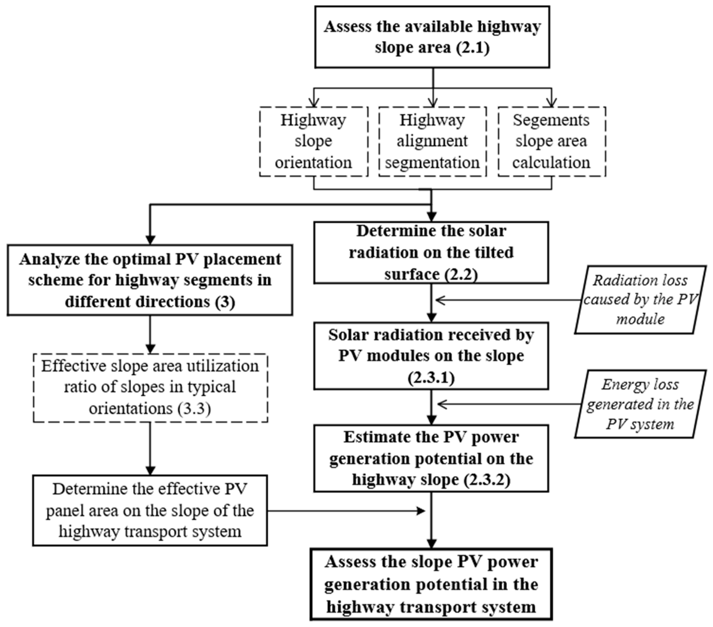
This study aims to develop a method to estimate the PV power generation potential of slopes in road transport systems. Considering the geometric characteristics and structure composition of highway infrastructure, the technical approach of the potential assessment is proposed and illustrated in Figure 1. The assessment starts with the segmentation of the highway alignment and a calculation of the available slope area, followed by an estimation of the inclined solar radiation. The factors causing the radiation and energy losses in the PV system are considered. The PV power generation potential of highway slopes can be determined after entering the highway geometric and radiation data and adopting the desirable placement scheme of the PV array.

2.1. Highway Segmentation and Slope Area Calculation

The effective solar radiation received on a highway slope is significantly affected by orientation. A slope facing due south is usually found to have the most exposure to solar radiation. However, the orientation of a highway slope surface changes constantly, as the shape and direction of the highway alignment varies along the road centerline. To facilitate the PV power generation potential evaluation, a highway alignment segmentation method is proposed, and a method for the calculation of the available slope area is established according to the spatial distribution characteristics of highway infrastructure.

2.1.1. Highway Slope Orientation Calculation

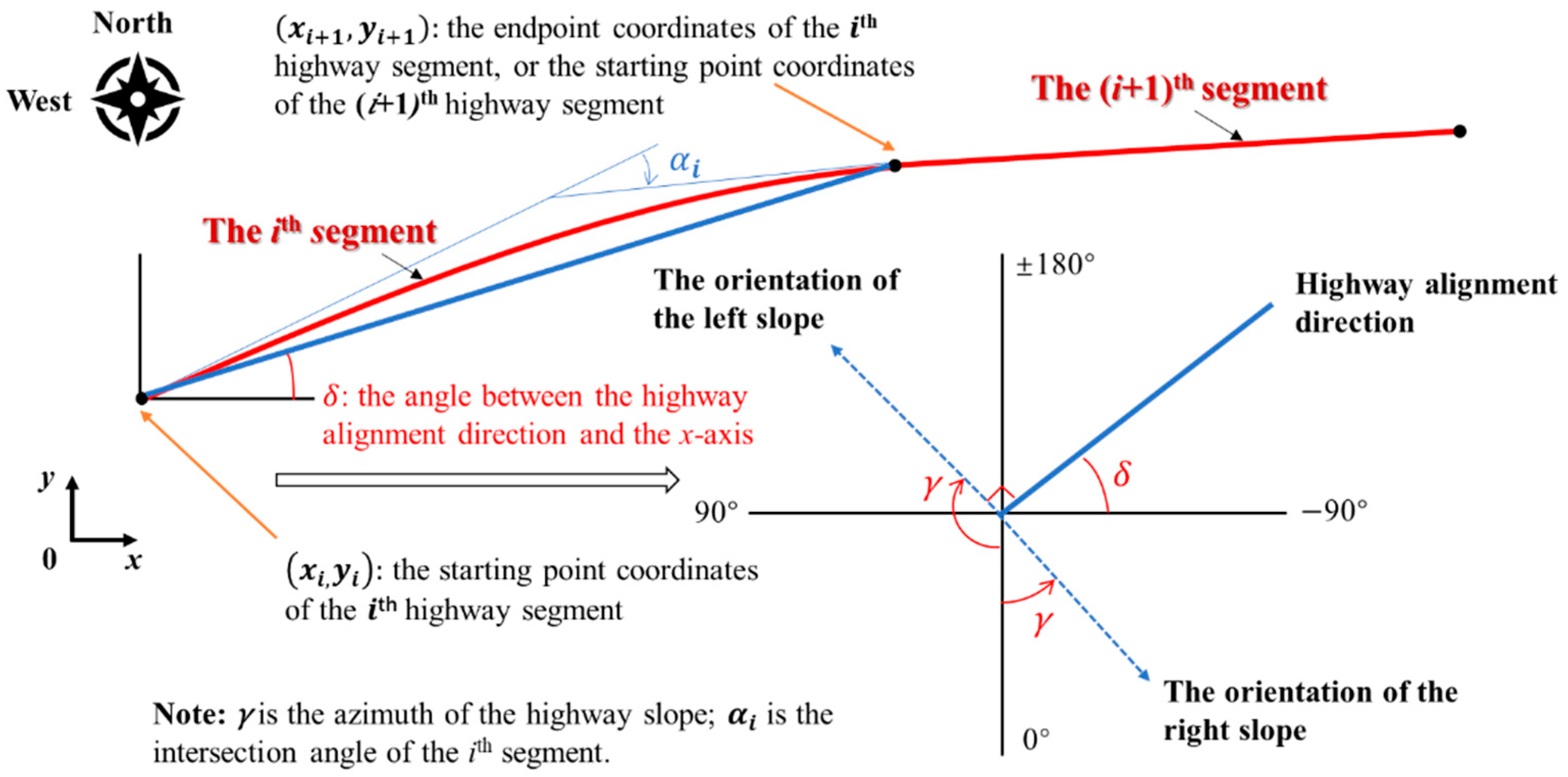
Generally, a highway alignment includes two primary types of sections, i.e., a straight-line section and a curve section. For straight-line sections or curves with small intersection angles (the angle between the tangents at the starting point and the ending point), the highway alignment direction can be determined using the coordinates of the starting and ending points. Subsequently, the slope orientation can be characterized by the azimuth of the slope (γ), which can be calculated according to the alignment direction. The highway alignment distribution and the slope orientation calculation methods are presented in Figure 2. The direction angle (δ) of a highway alignment can be calculated using Equation (1):
δ = t a n 1 ( | y i + 1 y i x i + 1 x i | )
where x i and y i are the x-axis and y-axis coordinates of the starting point of the i th alignment segment, respectively; x i + 1 and   y i + 1 are the ending point coordinates of the i th segment or the starting point coordinates of the ( i + 1 )th segment, respectively.
Once the direction angle of the highway segment is obtained, the azimuth of the corresponding slope can be determined based on the relation between the highway alignment direction and the slope orientation, as shown in 
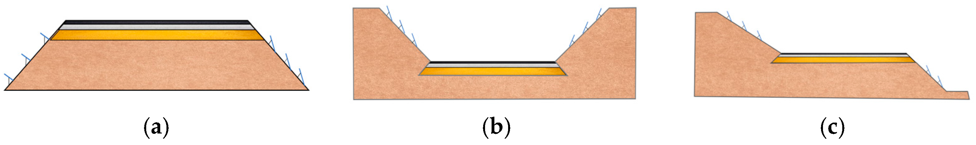
Figure 2. The highway subgrade is normally classified into three types, i.e., the fill-type, cut-type, and fill-and-cut-type subgrades, which are presented in Figure 3. The slopes of the fill-type and cut-type subgrades are usually symmetrical, indicating that the azimuth difference of the slopes on both sides is 180°. The PV power generation potential of a slope is significantly impacted by the type and orientation of the subgrade. Therefore, the slope orientation calculation method of the three kinds of subgrade was investigated to facilitate the potential assessment.
The slope azimuths of the fill-type subgrade in different directions were calculated, and they are presented in Table 1. For highway segments with the cut-type subgrade, the azimuths of the left and right slopes were found to be the same as those of the right and left slopes of the fill-type subgrade, respectively. Fill-and-cut subgrade slopes are the combination of the previous two types of slopes, and the slope azimuth can be determined accordingly. It should be noted that only the part higher than 5 m of the cut slope is considered for PV installation to reduce the influence of glare and reflection on drivers caused by the PV panels.

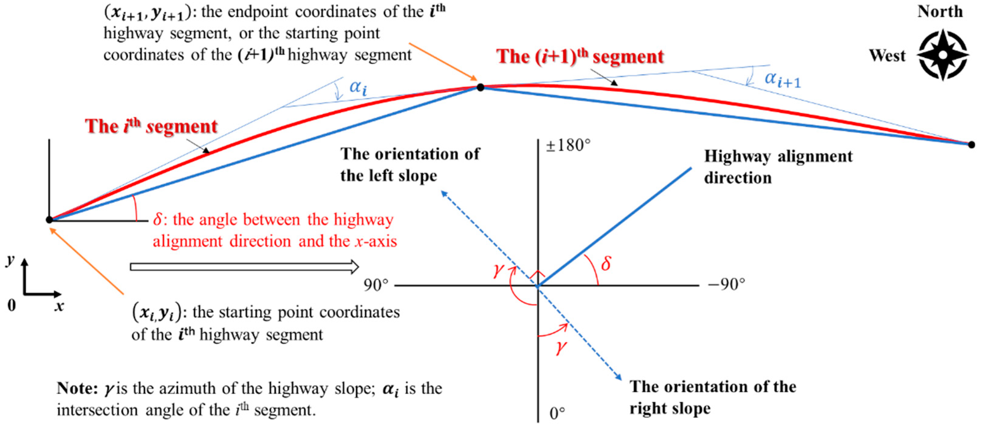
2.1.2. Highway Alignment Segmentation

For curve sections of a highway alignment with large intersection angles, alignment segmentation should be conducted to consider the impact of slope orientation variation on the effective solar radiation received on the slope. The curve sections should be divided into segments that can be approximately treated as straight lines, i.e., obtaining small intersection angles. A typical alignment segmentation scheme and slope orientation calculation method are presented in Figure 4. The highway direction determined by the starting and ending points of the divided segment and the corresponding slope azimuth shown in Table 1 could be adopted as the representative highway direction and slope azimuth.
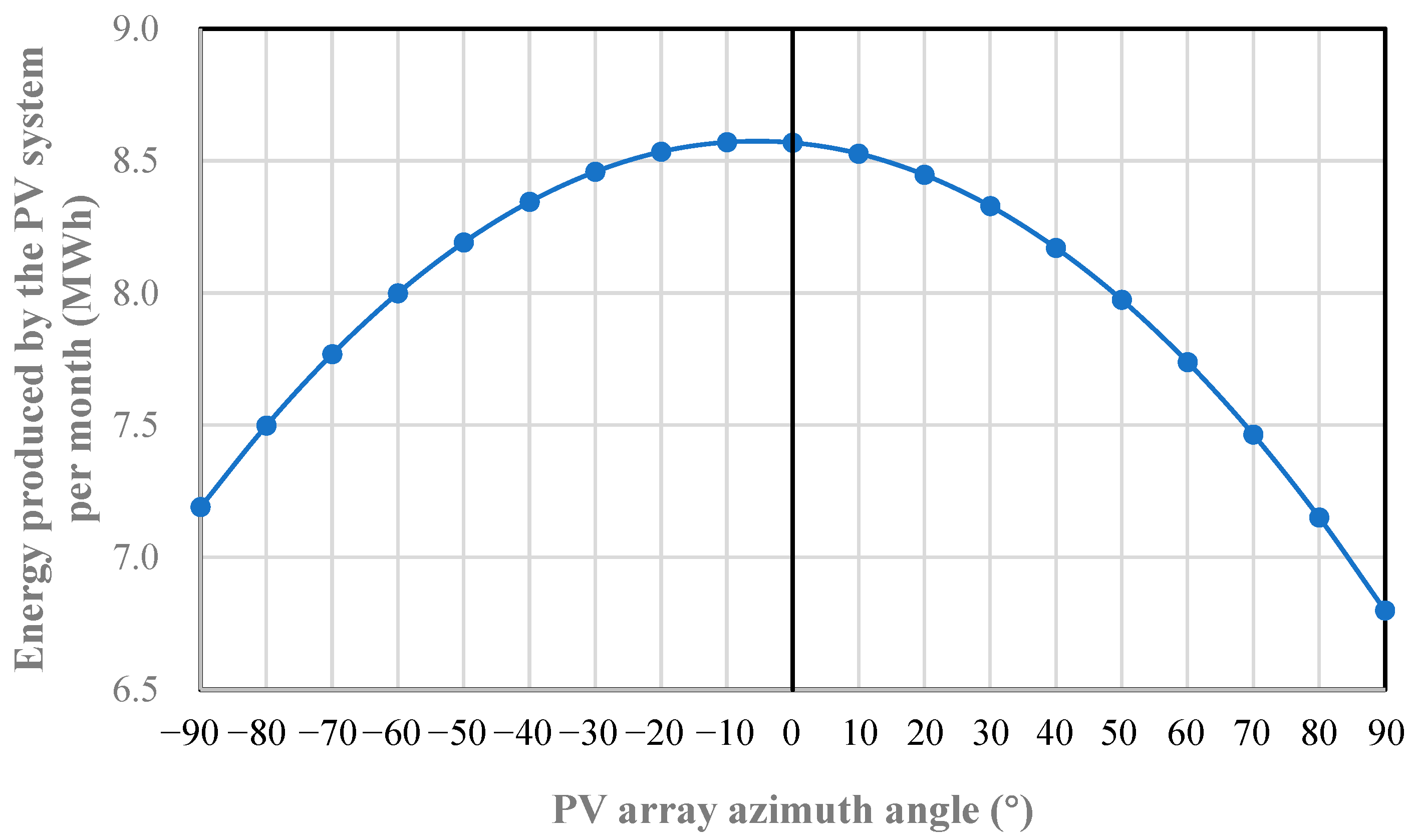
However, the number of divided segments will be too large if the intersection angle of each segment is too small. In contrast, the accuracy and reliability of the effective radiation calculation results will be significantly impacted if a curve segment with a large intersection angle is treated as a straight line. Therefore, it is necessary to determine the reasonable threshold of the intersection angle for the alignment segmentation. As the slope orientation is perpendicular to the highway direction, the intersection angle is equal to the change in the slope azimuth angle at the starting point and ending point. To determine the reasonable threshold, the influence of the slope azimuth variation on the power generation ability of the PV modules was analyzed utilizing the regression model between the PV array azimuth and the generated energy developed in the southern region of Slovakia by Bozikova et al. [24]. The model is demonstrated in Equation (2) and Figure 5.
E m ( γ ) = 0.1943 γ 2 2.1746 γ + 8568.8
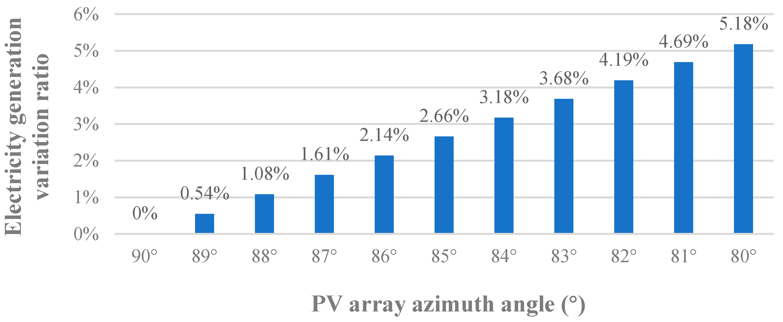
It can be observed in Figure 5 that the energy generation changing rate reaches the maximum value at an azimuth angle of 90 ° . Therefore, to evaluate the influence of azimuth variation on PV power generation, the variation ratios of the energy generated by the PV array with azimuth angles close to 90 ° were calculated, and they are shown in Figure 6. To ensure the accuracy and reliability of the power generation potential assessment, the energy generation variation ratio caused by the change in the slope azimuth in the divided segments should be controlled within certain levels based on the project requirements. If the variation ratio control level is set to 3%, the change in the azimuth angle should be less than 5° according to the results shown in Figure 6; this was selected as the threshold of the intersection angle for the alignment segmentation in this study.
Furthermore, after the threshold of the intersection angle is adopted, the segmentation length for the curve alignment sections can be determined according to Equation (3):
L i = r × α t × π 180 °
where r is the radius of the circular section in the curve alignment section m; α t is the threshold of the intersection angle, which was adopted as 5 ° in this study.
In a typical highway alignment, the curve section is commonly composed of a transition curve and a circular curve. The average curvature of the transition curve is smaller than that of the circular curve, resulting in a larger radius of curvature. Therefore, the segmentation length calculated with the transition curve radius will be larger than that calculated with the circular curve radius. To simplify the alignment segmentation of large-scale highway networks, the r in Equation (3) was conservatively adopted as the radius of the circular curve for the curve section.

2.1.3. Available Slope Area for PV Installation

The length of the slope area available for PV installation can be adopted as the straight-line length or the curve segment length. The width of the available slope area can be determined according to the height and grade of the highway slope. The average of the slope width at the starting point and ending point of the alignment segment was adopted as the representative width of the slope area, shown as follows:
B ¯ i = B i + B i + 1 2
where B ¯ i is the representative slope width of the i th highway segment; B i and B i + 1 are the slope width at the starting point and ending point of the i th highway segment, respectively, which can be calculated as follows:
B i = Δ H i s i n ( t a n 1 1 m i )
where Δ H i and 1 / m i are the slope height and slope grade at the starting point of the i th segment, respectively.
The available slope area for PV installation can be determined based on Equation (6) after the length and width are obtained:
S i = B ¯ i × L i
where S i   is the available slope area of the i th highway segment for PV installation.

2.2. Solar Radiation Estimation on a Tilted Surface

The solar radiation received on a tilted surface is composed of three parts, i.e., the direct solar radiation, the sky-scattered radiation, and the ground-reflected radiation [25,26], which is shown as follows:
H T = H b T + H d T + H r T
The direct solar radiation on a tilted surface H b T can be calculated as follows:
H b T = H b R b
where R b [27] is the direct light enhancement coefficient, which can be calculated as follows:
R b = max [ 0 , c o s θ i s i n α ]
where θ i and α are the solar incidence angle and solar elevation angle in degrees, respectively, which can be determined as follows:
θ i = c o s 1 [ s i n φ c o s β + s i n φ s i n β c o s ( γ s u n A ) ]
α = s i n 1 ( s i n φ c o s δ + c o s φ c o s δ c o s ω )
where A is the sun azimuth in degrees; φ is the local latitude in degrees; and ω can be expressed as follows:
ω = ( t 12 ) × π 12 m ( L g t L g ) × π 180
where t is the time zone time in a 24 h clock; m is the model coefficient, which adopts 1 and −1 for the eastern and western hemispheres, respectively; L g t is the time zone center longitude in degrees;   L g is the local longitude in degrees; and δ s u n [28] is the sun declination in degrees, which can be determined as follows:
δ s u n = 23.45 × s i n ( 360 × 284 + n 365 )
where n is the order of days in a year ranging from 1 to 365.
The amount of scattered radiation on a tilted surface H d T can be determined based on the Hay model [29], as shown in Equation (14):
H d T = H d [ H b H O R b + 1 2 ( 1 H b H O ) ( 1 + c o s β ) ]
where H O is the solar radiation at the outer level of the atmosphere in kWh / m 2 , which can be calculated as follows:
H O = 24 π H S C [ 1 + 0.033 c o s ( 360 n 365 ) ] ( π ω 180 s i n φ s i n δ s u n + c o s φ c o s δ s i n ω )
where n, ω, φ, and δ have the same meanings as illustrated above.
The amount of ground-reflected radiation on a tilted surface H r T [30] can be determined using Equation (16):
H r T = 1 2 ρ ( H b + H d ) ( 1 c o s β )
where ρ is the average reflectivity of the ground, which is generally adopted as 0.15; H b , H d , and β have the same meanings as clarified above.
Therefore, the unit area solar radiation received on a tilted surface can be determined based on Equations (7)–(16) using geographic location data, such as longitude and latitude; solar radiation data on the horizontal plane, such as H b and H d ; and the inclination angle and the azimuth angle of the tilted surface.

2.3. PV Power Generation Potential Assessment

Further analysis in the highway slope PV power generation potential assessment method can be conducted once the available slope area and solar radiation are obtained. However, the radiation loss of the PV modules and the energy loss in the PV array’s distributed microgrid system will significantly affect the PV power generation potential. Hence, related factors are considered in the assessment process and are discussed in this section.

2.3.1. Solar Radiation Received by PV Modules

Ideally, the calculation of the PV module’s received solar radiation mainly considers the azimuth and tilt angles of the module. However, a considerable solar radiation loss will be generated due to occlusion and light transmittance. Therefore, the near shading, far shading, and IAM losses should be accounted for when determining the PV module’s received solar radiation. The impacts of the three loss sources and the quantitative calculation method are demonstrated below.
(1)
Near shading and Far shading
Near shading and far shading are mainly composed of remote near shading and far shading and close near shading and far shading. Remote occlusion generally considers nearby mountains or other distant but large objects. The solar radiation received by the photovoltaic arrays is reduced to a certain extent due to the huge volume and the relative geographical location to the slope. Close near shading and far shading include two aspects, i.e., the occlusion of the PV panel itself and the surrounding obstacles. To reduce close occlusion, a certain interval between the PV panels and a certain distance from the surrounding obstacles are required for the installation of the PV array system.
In this study, the remote occlusion reduction coefficient Kd was used to quantify the radiation loss caused by the occlusion of remote objects. In a flat terrain area, the remote occlusion effect is low, and Kd can be adopted as 1. In complex terrain or mountainous areas, the remote occlusion effects on the PV modules are complex, and it is advised to determine Kd based on local experience or onsite measurements using radiometers. The close occlusion reduction coefficient Kn was utilized to represent the shading effects of the PV panels and the highway slope. The PV array placement scheme and the cross-section type of the highway subgrade significantly affect the occlusion of PV modules. Therefore, the value of Kn is suggested to be determined by simulating the PV power generation under certain placement schemes in software such as PVsyst7.2.
(2)
The IAM loss
The IAM loss refers to the process of reducing the actual total solar radiation received due to the reflection and scattering of the solar panel during the process of solar radiation entering the PV panel from the air. The radiation loss can be quantified via natural light reflectivity (R), which is primarily related to the reflection ability of the optical material, the incidence angle, and the packaging glass material of the PV module. Common calculation models include Fresnel’s law, the ASHRAE model, and the Sandia model. Fresnel’s law [31,32] was used in this study, and the formula is as follows:
R = 1 2 [ s i n 2 ( θ i θ t ) s i n 2 ( θ i + θ t ) + t a n 2 ( θ i θ t ) t a n 2 ( θ i + θ t ) ]
where R is the reflectivity of natural light; θ i is the solar incidence angle in degrees; and θ t is the reflection angle of the incident light in degrees.
Generally, the sum of transmittance and reflectivity is 1, and the transmittance (T) will significantly affect the absorption of direct solar radiation on a tilted PV panel ( H b T ). Therefore, the effective direct solar radiation ( H b t ) received by the PV panel can be determined using Equation (18):
H b t = H b T × T
where T is the transmittance of natural light, which can be calculated as follows:
T = 1 R
Accordingly, the effective solar radiation on tilted PV modules can be obtained by utilizing Equation (20):
H A = H t × K d × K n
where H A is the effective solar radiation on tilted PV modules; K d is the remote occlusion reduction coefficient; and H t is the solar radiation received by tilted PV modules considering the IAM loss, which can be determined as follows:
H t = H b t + H d T + H r T
where H d T is the sky-scattered radiation on a tilted surface; H r T is the ground-reflected radiation on a tilted surface.

2.3.2. Theoretical Power Generation of PV Module and Actual Power Generation of PV System

After obtaining the effective solar radiation received by an inclined PV module, the theoretical power generation can be determined by considering the photoelectric conversion efficiency of the PV module with the following equation:
E L = H A × η m
where E L is the theoretical power generation of tilted PV modules, kWh / m 2 ; η m is the photoelectric conversion efficiency, which is adopted as 0.15 for conventional crystalline silicon photovoltaic modules.
PV array systems with many modules will have a power loss caused by temperature changes in the modules, the power loss in the inverters, and the PV module performance decay. The evaluation method for these factors is discussed and illustrated below.
Firstly, temperature changes in the PV modules will affect the photoelectric conversion efficiency [33,34], which can be evaluated using the temperature correction coefficient shown in the following equation:
η T = ( T c 25 ) × λ T
where   η T is the temperature correction coefficient; λ T is the maximum power temperature coefficient of the PV module; and T c is the temperature of the PV module.
Secondly, the inverter loss is mainly caused by the energy loss during the operation of the inverter, which is related to the technical parameters and operating conditions of the inverter itself and is evaluated with the inverter loss correction coefficient K t . For typical inverters with a nominal AC power of 60 k w a c , the number of MPPTs of 16, and the inverter capacity ratio is 1.27; according to our calculations in PVsyst, K t is generally adopted as 0.98.
Thirdly, the power generation ability of PV modules will decrease as the module performance decay accumulates with time, which can be evaluated with the PV module performance decay correction coefficient K r . Generally, the average annual power attenuation rate of conventional crystalline silicon photovoltaic modules is in the range of 0.8~0.9%. Combining the above correction factors and the theoretical power generation of PV modules, the actual power generation of the PV system can be obtained with the following equation:
E S = E L × η T × K t × K r
where E S is the actual power generation of the PV system, kWh / m 2 ; K t is the inverter loss correction coefficient; and K r is the PV module performance decay correction coefficient.
Based on the above analysis, the actual power generation of the PV system can be calculated based on the solar radiation data on the horizontal plane and the placement conditions. The comprehensive formula is as follows:
E S = [ ( H b T × T ) + H d T + H r T ] × K d × K n × η m × η T × K t × K r
where all symbols used in the above formula have the same meanings as illustrated above.

2.3.3. Assessment of Total Solar Power Generation Potential

By integrating the above key steps of the solar power generation evaluation, a basic assessment method for the PV power generation potential of highway slopes can be proposed as follows: (1) segment the alignment of highways in the system; (2) calculate the available slope area for the PV array placement of each highway segment; (3) calculate the effective radiation received by the tilted PV arrays on the slopes of each highway segment considering the radiation loss caused by the PV module; (4) calculate the effective power generation of the PV array on the slope of each highway segment considering the energy loss generated in the PV system; and (5) calculate the total solar power generation potential of the highway slope in the transport system.
Therefore, the total solar power generation potential of a highway slope can be determined based on Equation (26) as follows:
E T o l = E T L + E T R = i = 1 i = n E S i × S i + j = 1 j = n E S j × S j = i = 1 i = n H t i × K d i × K n i × η m i × η T i × K t i × K r i × S i + j = 1 j = n H t j × K d j × K n j × η m j × η T j × K t j × K r j × S i
where E T o l is the total solar power generation potential on highway slopes, kWh ; E T L and E T R are the total solar power generation potential on the left and right highway slopes, respectively, kWh ; i and j are the left slope ID and right slope ID of different highway segments, respectively; E S is the unit area actual power generation on the slope, kWh / m 2 ; S is the available slope area of different highway segments, m 2 ; H t is the solar radiation received by a tilted PV module considering the IAM loss; K d is the remote occlusion reduction coefficient; K n is the close occlusion reduction coefficient; η m is the photoelectric conversion efficiency; η T is the temperature correction coefficient; K t is the inverter loss correction coefficient; and K r is the PV module performance decay correction coefficient.

3. The Placement Scheme of PV Array on Highway Slopes

Within the available highway slope area, the orientation and tilt angle of the PV array placement have crucial impacts on the power generation potential. Additionally, the divided highway segments generally run in different directions, which results in various slope orientations. The desirable PV array placement scheme should be different for differently orientated slopes. To estimate the maximum solar power generation potential of a highway slope, the optimal PV array placement scheme needs to be determined for slopes of highway segments running in different directions.

3.1. The Desirable Tilt Angle for Conventional Placement Orientation

PVsyst is a piece of photovoltaic system design and simulation software that can predict the power generation of photovoltaic modules based on the layout and layout scale. At the same time, the software can design the electrical system of a photovoltaic array and handle solar radiation data of different areas. Simulations using this software have a high reliability. Therefore, we used the software PVsyst version 7.2 to determine the ideal slope inclination angle for PV modules installed on highway slopes.
According to PVsyst7.2, the best tilted angle can be derived with the input of the longitude, the latitude, the placement orientation, the total radiation, the diffuse radiation, the temperature, and the technical parameters of the PV system. Generally, the PV array is installed in the same orientation as the slope, which is the conventional placement orientation. Four typical road directions were considered in this study, i.e., due south, due east, 45° north by east, and 45° north by west, which are shown in Figure 7. Accordingly, the slope orientation could be determined based on the method illustrated in Section 2.1.1, and the optimal tilt angle could be simulated through PVsyst7.2.
Taking Xi’an (108.9° E, 34.3° N) as an example, a 70 m long straight-line east–west fill-type road was selected to illustrate the method of determining the desirable PV tilt angle on a slope. The slope height and slope angle were 6 m and 30°, respectively. For the south-facing slope, the azimuth angle of the PV modules was 0°. The power generation of the PV array on the south slope was simulated in PVsyst7.2, and the optimal tilt angle for the whole year was determined to be 26°. The following settings and parameters were adopted in the simulation process: a 1.640 m long and 0.992 m wide monocrystalline silicon PV module with a 250 w p rated power and a 26V rated voltage, and an inverter with a 7.5 kW rated power and a 150–750 V working voltage. Based on the slope dimensions, four PV panels were designed and placed on the slope along the road direction, as shown in Figure 8. For each panel, there were 4 and 19 modules along the length and width directions of the slope, respectively. The intervals between the panels along the length and width directions were adopted as 2.4 m and 1.2 m, respectively. Accordingly, 304 PV modules and 8 inverters were adopted, resulting in a total nominal power of 76 k w p .
Similarly, the optimal tilt angles of PV arrays on the slopes of roads in typical directions could be simulated and derived using PVsyst7.2, and they are shown in Table 2. However, the desirable PV array placement may not always be in the same orientation as the target slope. PV panels placed at an azimuth angle different from the conventional orientation may produce a larger power generation for roads running in different directions. Therefore, the desirable PV placement scheme for slopes in different orientations should be further investigated.

3.2. The Desirable PV Array Placement Scheme

3.2.1. Placement Scheme for East–West Slopes

The azimuth angles of the southern and northern slopes of the east–west highway were found to be 0° and 180°, respectively. For the southern slope, there were mainly three kinds of placement schemes, as shown in Figure 9. In placement scheme 1, the PV panels were installed with the longer side parallel to the road direction, and tilt angles of 0° and 26° relative to the horizontal plane were simulated using PVsyst7.2. In placement schemes 2 and 3, the PV panels were placed with the longer side perpendicular to the road direction, and the tilt angle was changed relative to the slope surface by rotating along the western and eastern panel edges, respectively. The tilt angles of 0°, 10°, 20°, and 30° were considered in the power generation simulation in PVsyst7.2 for schemes 2 and 3. Therefore, seven placement schemes were proposed for the southern slope of the east–west highway, and the power generation simulation results are shown in Table 3, which indicates that scheme 1-2 obtains the highest power generation potential.
For the northern slope of the east–west highway, four kinds of placement schemes were proposed, and they are illustrated in Figure 10. In placement scheme 1, the PV panels were installed with the longer side parallel to the road direction, and a 0° tilt angle relative to the horizontal plane was simulated using PVsyst7.2. In the second type of placement, the lower row of PV panels in scheme 1 was removed to consider the shading effect of the higher row of PV panels. In schemes 3 and 4, the PV panels were placed with the longer side perpendicular to the road direction, and the tilt angle was changed relative to the slope surface by rotating along the western and eastern panel edges, respectively. The tilt angles of 0°, 10°, 20°, and 30° were considered in the power generation simulation in PVsyst7.2. Therefore, nine placement schemes were proposed for the northern slope of the east–west highway, and the simulation results are presented in Table 4.
It can be seen in Table 4 that scheme 2 illustrated the highest power generation efficiency, followed by scheme 1. However, the overall installed PV panel area of scheme 2 was only half of that of scheme 1, resulting in a lower power generation potential. Therefore, placement scheme 1 is recommended for the northern slope.

3.2.2. Placement Scheme for Slopes of 45° North by East Highway

For highways in the direction of 45° north by east, the azimuth angles of the southern-side slope and the northern-side slope were found to be −45° and 135°, respectively.
Firstly, the PV placement scheme on the southern slope was analyzed. Two types of PV placement methods were proposed, and they are shown in Figure 11 to explore the maximum solar energy generation potential of the road slope. In the first type of method, the PV panels were installed with the longer side parallel to the road direction, and the optimal tilt angle of 20° was simulated in PVsyst7.2. In the second type of method, the PV panels were placed with the longer side perpendicular to the road direction, and the tilt angle was changed by rotating the panel along the southern edge of the panel. The tilt angles of 0°, 10°, 20°, and 30° relative to the slope surface were simulated in PVsyst7.2. Accordingly, five placement schemes were proposed, and the power generation simulation results are shown in Table 5. Scheme 2-2 showed the highest power generation ability, which is suggested for PV installation on the southern slope.
For the northern slope, the two placement methods of the southern slope were also adopted. Additionally, the 0° tilt angle was considered in the first type of placement method, and the lower row of PV panels was removed due to the serious occlusion on the north-side slope, which is placement scheme type 2 shown in Figure 12. Therefore, six placement schemes were put forward, and the power generation simulation results are presented in Table 6. Placement scheme 2 illustrated the highest power generation potential but a lower total installed PV panel area than scheme 1. Therefore, scheme 1 is recommended when a higher overall power supply is required, and scheme 2 is more suitable if a higher power generation efficiency is desired.

3.2.3. Placement Scheme for Slopes of 45° North by West Highway

The slope azimuth angles of highways in the direction of 45° north by west were found to be −135° and 45°, respectively. The 45° north by west highway slopes have proposed PV array layout schemes similar to those of the 45° north by east highway slopes shown in Figure 11. The power generation simulation results of the southern and northern slopes are shown in Table 7. The placement scheme 2-2 is suggested for the southern slope, and scheme 1 or 2 is advised for the northern slope.

3.2.4. Placement Scheme for Slopes of the North–South Highway

The azimuth angles of the west and east slopes of the north–south direction highway were found to be −45° and 45°, respectively. As the slopes on the two sides are symmetrical, similar PV placement schemes could be applied on each side. Taking the west slope as an example, three kinds of placement methods were considered, and they are shown in Figure 13. In the first type of placement method, the PV panels were installed with the longer side parallel to the road direction, and a 0° tilt angle was simulated in PVsyst7.2 to estimate the power generation. In the second type of placement, the lower row of PV panels of the first type of scheme was removed to consider the shading effect of the higher panels. In the third type, the PV panels were installed with the longer side perpendicular to the road direction, and the tilt angles of 0°, 10°, 20°, and 30° relative to the slope surface were simulated. Therefore, six placement schemes were designed for the west slope or the east slope, and the power generation simulation results are presented in Table 8.
It can be seen in Table 8 that schemes 3-2 and 3-3 had the highest power generation potential, and scheme 2 illustrated the highest power generation efficiency for both sides of the north–south highway slope. Therefore, placement schemes 3-2 and 3-3 are recommended for general application conditions, while scheme 2 is suggested for scenarios where the power generation efficiency takes precedence over design considerations.

3.3. Effective Slope Area Utilization Ratio

It can be inferred from the placement scheme analysis of the slopes of highways running in different directions that the desirable PV array layout design varies with the change in the slope orientation. To facilitate the estimation of the PV power generation potential in highway engineering, the effective slope area utilization ratio (ESUR) is put forward and defined as the ratio of the installed PV modules’ area to the slope area. The ESURs of the optimal placement schemes for slopes running in the typical directions were calculated, and they are summarized in Table A1. During the application stage, engineers could take the ESURs of slopes in the typical orientations as references to estimate the potential PV module area on the highway slopes of local projects.

4. Case Study of PV Power Generation Potential Assessment

(1)
Collection of geographic and climate information
In this case study, the slope solar power generation potential of a highway in Chang’an District, Xi’an City, China, was calculated. The research site is located near 108.93° E and 34.17° N, and the typical annual horizontal radiation of Xi’an was selected as the horizontal solar radiation data for this example, which is presented in Table 9.
(2)
Highway alignment geometric data collection and segmentation
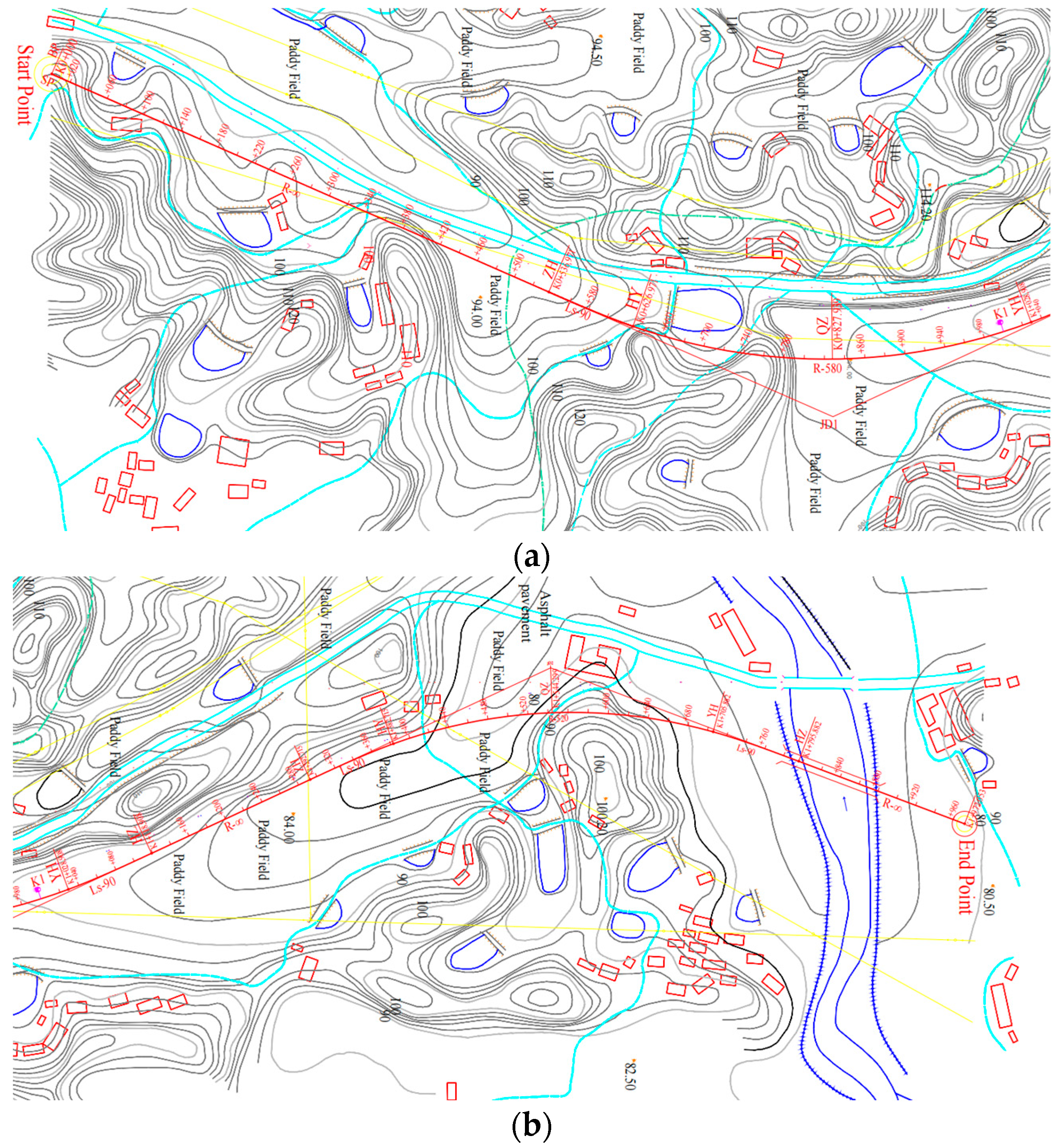
For the convenience of explanation, this paper only took a 1.97 km long section of the expressway as an example to illustrate the calculation method of the solar power generation potential of highway slopes. The horizontal alignment design of the selected highway section is shown in Figure 14. There are four transition curves and two circular curves in the horizontal alignment. The length of the transition curves, the radius of the circular curves, the stake number, and the coordinates could be obtained from the design documents. The length of each transition curve is 90 m, and the radii of the circular curves are 520 m and 580 m.
Based on the alignment geometric data, highway segmentation can be conducted according to the method presented in Section 2.1.2. It is a straight line from the starting point to station K0 + 536.97 of this highway section, which was set as the first segment. The first transition curve and circular curve follow after station K0 + 536.97. According to the principle that the intersection angle of the segmented curve should be less than 5 ° , the segmentation length was determined to be 50.61 m for the first circular curve. Similarly, the segment length of the second circular curve was calculated as 45.37 m. Accordingly, the selected highway section could be divided into 27 segments, and the geometric data are shown in Table A2. Furthermore, the highway direction and the slope azimuth angles could be determined based on Equation (1) and Table 1, which are presented in Table A2.
(3)
Calculation of available slope area of the highway segments
Taking the first highway segment as an example, it is necessary to consider the length, the width, and the proportion of the slope that are required for the PV array placement. Since there is a 180 m long retaining wall installed along the left slope of the first segment based on the design document, this part of the slope was considered for solar energy utilization in this study. As the slope widths at the two ends of the first segment are 2.93 m and 15.42 m, the average slope width could be determined to be 10.35 m according to Equation (4). The length of the slope could be calculated as the station number difference between the two ends of the segment, and it was 536.97 m. By subtracting the length of the retaining wall, the effective slope length should be 356.97 m. Accordingly, the available slope area could be calculated based on Equation (5), and it was 3694.64 m 2 . Therefore, the available slope area of all segments could be determined, and they are illustrated in Table A3.
(4)
The optimal placement scheme and area of the PV array for highway segments
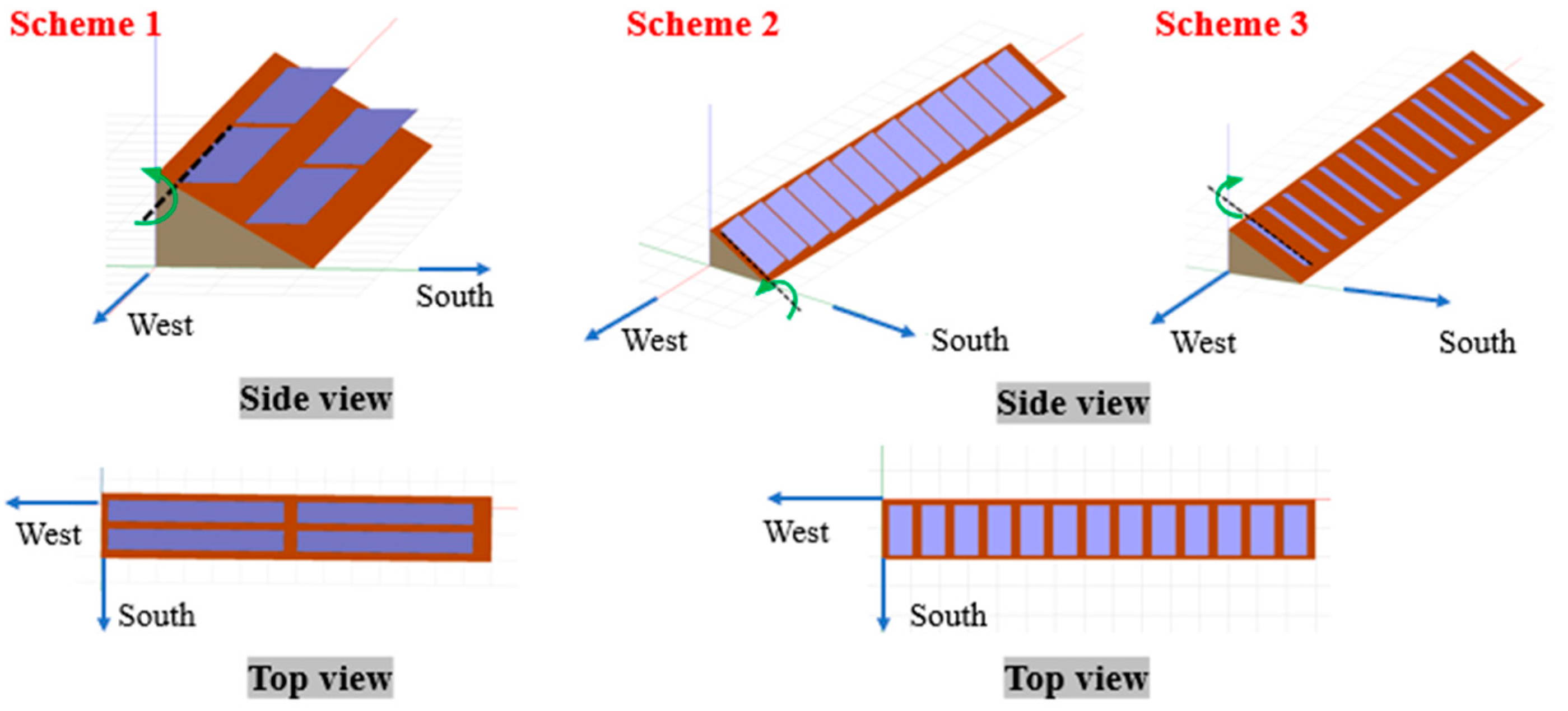
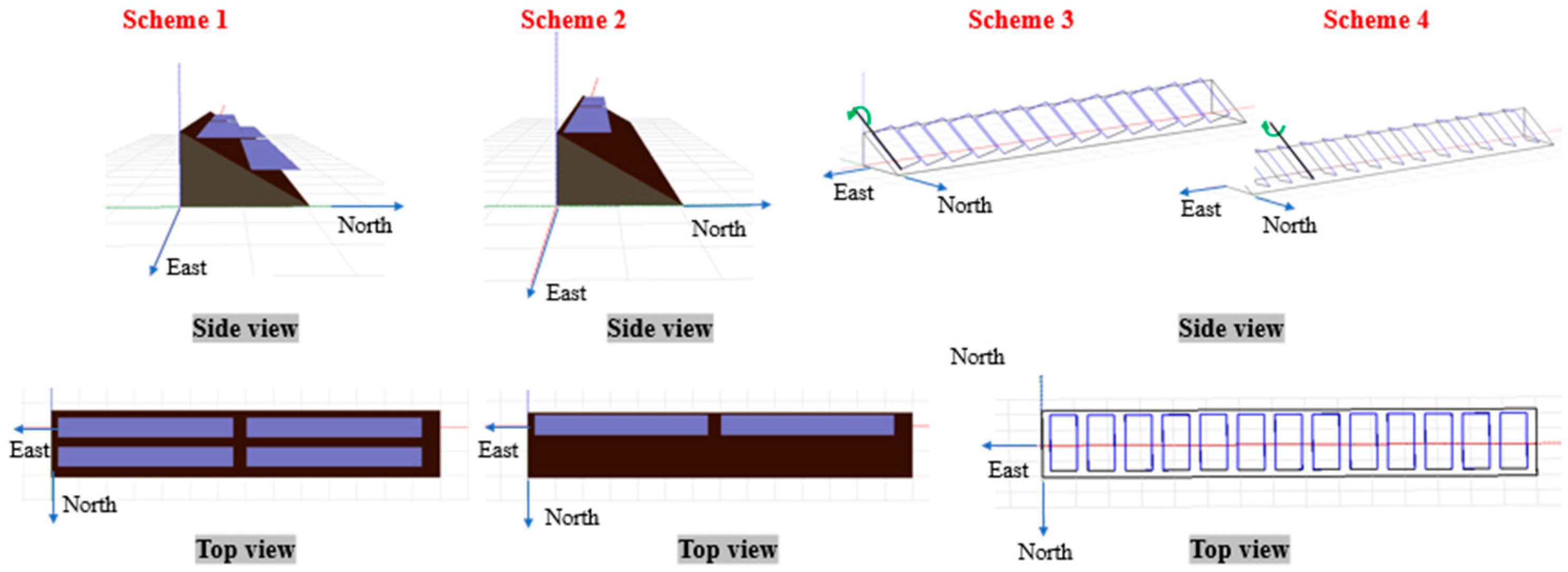
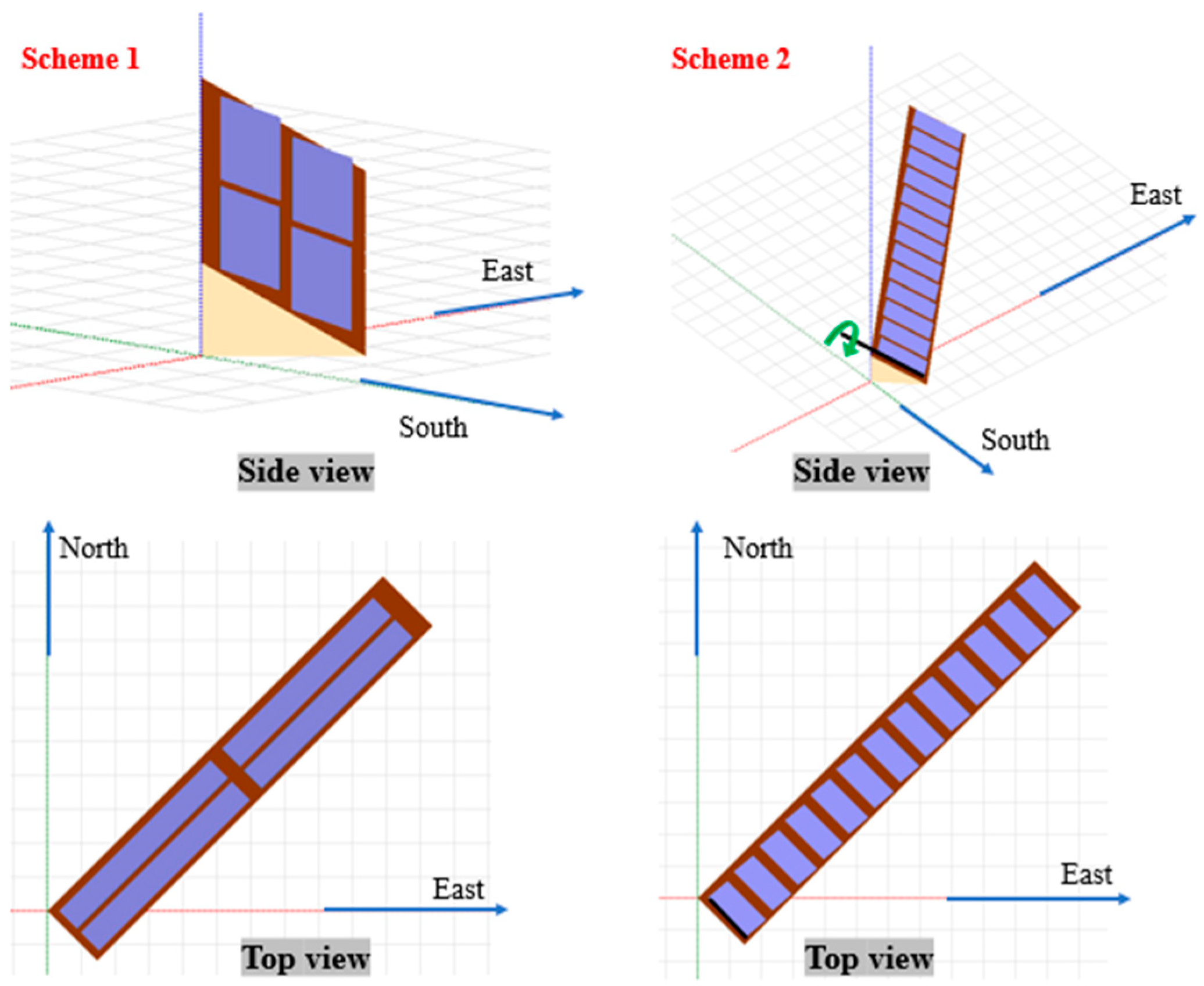
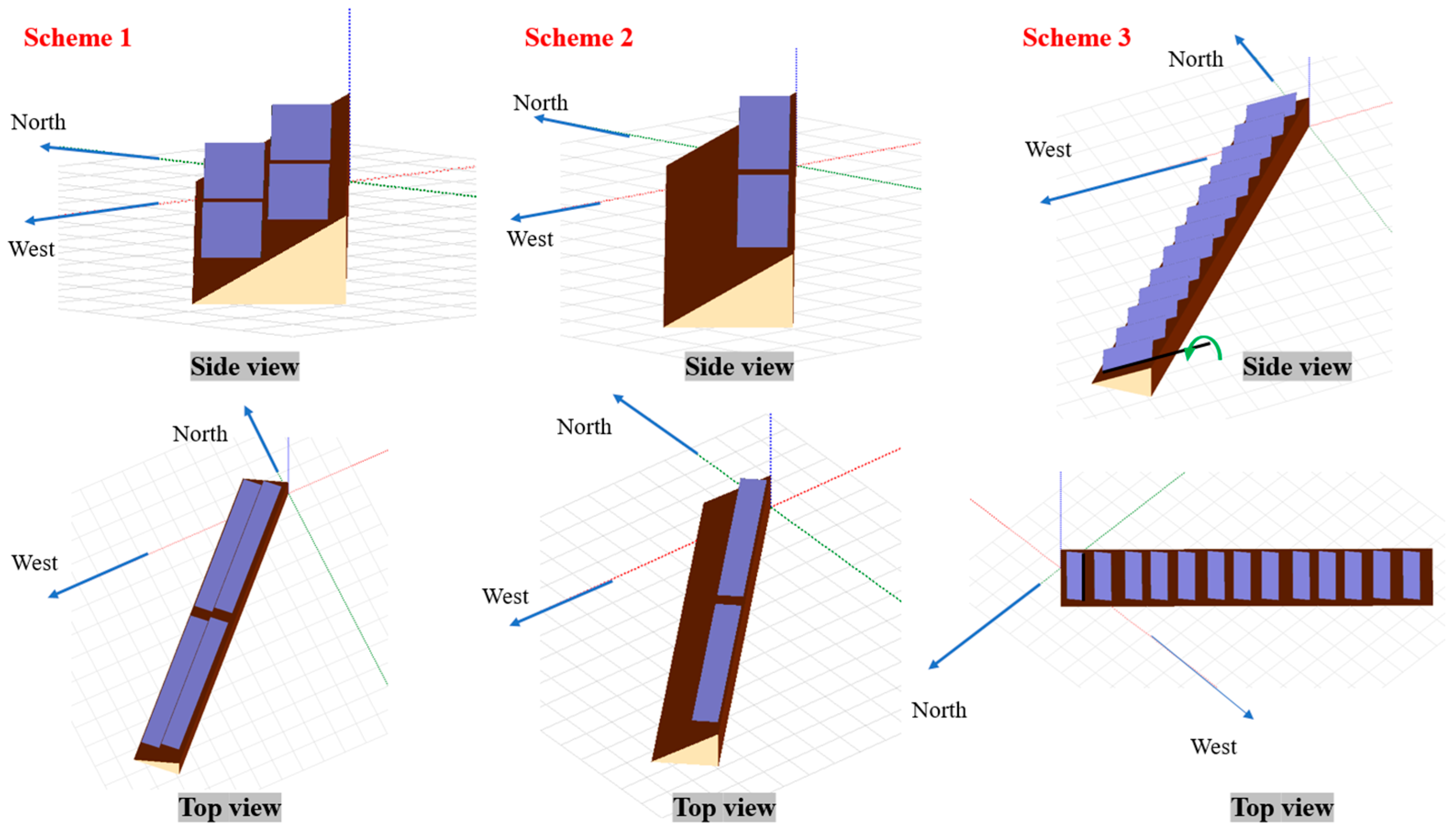
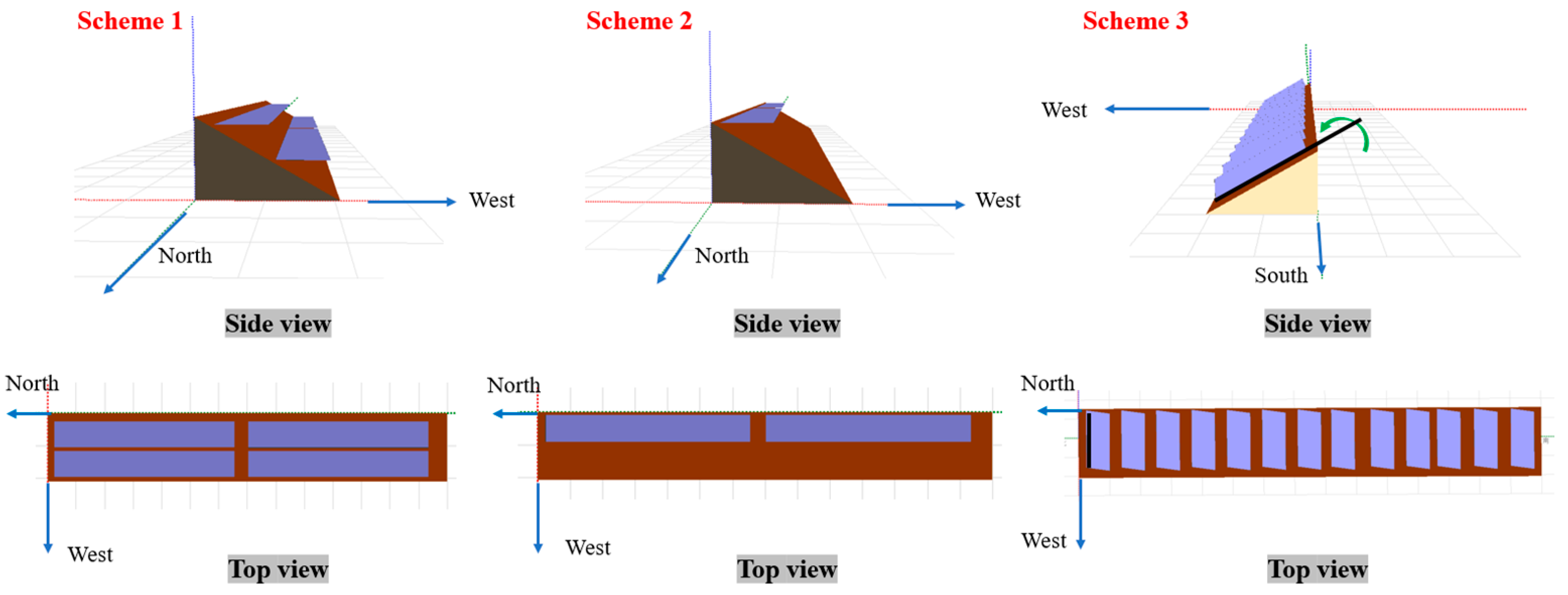
The optimal placement schemes of the highway segments with different slope orientations could be selected based on the recommended schemes presented in Table 9. Taking the first segment, for instance, the azimuth of the right slope is 23.69° (as shown in Table A2), which is between 0° and 45°. Therefore, the power generation was simulated with the placement schemes “① + 26°” and “① + 20°”. The simulation results show that the scheme “① + 26°” had a higher power generation, and this was selected as the desirable placement scheme for the right slope of the first segment. Subsequently, the area of the PV array that could be placed on the slope could be determined according to the effective slope area utilization ratio of the corresponding installation scheme shown in Table 9. Accordingly, the optimal placement scheme and area of the PV array for slopes of different highway segments were determined, and they are documented in Table A4.
(5)
The theoretical and actual solar radiation received by per unit PV panel area
The theoretical unit area solar radiation on the tilted PV array surface could be calculated based on the location of the project, the placement scheme of the PV array, and the solar-radiation-related coefficients according to the method illustrated in Section 2.2. Thereafter, the actual solar radiation received by the PV panel could be obtained by subtracting the near shading, far shading, and IAM losses according to the method presented in Section 2.3.1. As the selected section of the highway is in the flat terrain area, the remote occlusion effect Kd was adopted as 1. The close occlusion reduction coefficient Kn and the transmittance of natural light on the PV modules were determined by simulating the PV power generation under the selected placement schemes in PVsyst7.2. Accordingly, the values of the theoretical and actual solar radiation received by per unit PV panel area on the slopes of different highway segments were calculated, and they are presented in Table A5.
(6)
Calculation of the actual power generation of the PV array on highway slopes
The theoretical power generation of the tilted PV modules could be determined according to Equation (13), utilizing the actual unit area solar radiation results shown in Table A5, and the photoelectric conversion efficiency was adopted as 0.15 in this study. Afterwards, the actual power generation of the PV system could be calculated using Equation (15). As the temperature of the PV module varies with time during the year, the yearly average value of the temperature correction coefficient η T was determined by simulating the power generation of the 27 highway segments and calculating the temperature loss in PVsyst7.2. Therefore, η T was adopted as 0.95 in this study. The inverter loss correction coefficient K t was adopted as 0.98 to represent general application conditions, while the PV module performance decay correction coefficient was not considered since the long-term power generation potential was not the main focus of this case study. Therefore, the theoretical and actual power generation potentials of the PV system on the slopes of the selected highway section could be determined, and they are shown in Table A6.
(7)
Assessment of the solar power generation potential of the selected highway section
After a comprehensive analysis and calculations of the case study, the available slope area for the PV array installation, the actual unit area solar radiation received on the tilted PV panels, and the actual unit area power generation of the PV array on the slopes of the 27 highway segments were obtained. Therefore, the actual annual power generation potential of the selected highway section could be further determined according to Equation (17). The assessment results of the solar power generation on the slopes of different highway segments are illustrated in Table A7, and the overall solar power generation potential of the studied highway section was found to be 3,896,061.68 kWh in total.

5. Summary and Conclusions

The assessment method of the PV power generation potential of highway slopes was established by considering the geometric characteristics of highways and the desirable PV array placement scheme. The available highway slope area was determined based on the highway segmentation results. The effective power generation potential per unit of PV panel area was derived by subtracting the radiation loss of the PV modules and the energy loss in the PV system. Accordingly, the overall power generation potential of the highway slopes could be acquired based on the available slope area and effective solar power generation efficiency results of all highway segments. Finally, a case study was provided to illustrate the application of the proposed assessment method. The primary conclusions of the study are listed as follows:
(1)
Highway segmentation should be performed based on the change in slope orientation and the effects on solar power generation. The intersection angle threshold of 5° corresponding to a 3% variation level of the solar power generation was adopted for the alignment segmentation in this study.
(2)
The near shading, far shading, and IAM losses should be considered in radiation loss calculations, and the correction coefficients of the temperature, the inverter loss, and the PV module performance decay should be applied when calculating the actual unit area PV power generation potential.
(3)
The optimal PV array placement scheme varies with the slope orientation, which was determined through the power generation simulation in the software PVsyst (version 7.2). The corresponding effective slope area utilization ratio was calculated and is documented in Table A1 to serve as a reference for future solar power generation potential assessments.
(4)
The proposed method was applied in a potential assessment case study of one 1.97 km long highway section in Xi’an City, China. The overall annual power generation potential of the highway section was found to be 3,896,061.68 kWh.

Author Contributions

Conceptualization, A.S. and L.H.; methodology, Z.H.; software, W.Z.; validation, Z.H., W.Z., and R.W.; formal analysis, Z.H.; investigation, W.Z.; resources, A.S. and L.H.; writing—original draft preparation, W.Z.; writing—review and editing, Z.H. All authors have read and agreed to the published version of the manuscript.

Funding

This research was funded by the National Key R&D Program of China, grant number 2021YFB2601300.

Institutional Review Board Statement

Not applicable.

Informed Consent Statement

Not applicable.

Data Availability Statement

Data are presented in the article.

Conflicts of Interest

The authors declare no conflict of interest.

Abbreviations

PV, photovoltaic; PGS, power generation system; PGP, power generation potential; ESUR, effective slope area ratio; PVsyst, photovoltaic systems; GIS, geographic information system; IAM, incident angle modifier.

Nomenclature

δ the angle between the highway alignment direction and the x-axis
E m the monthly average electricity generated by the PV array, kWh
γ the azimuth angle of the PV array surface ranging from 90 ° to 90 ° , which represents the azimuth of the highway slope
H T the total amount of solar radiation received on a tilted surface, kWh / m 2
H b T the direct solar radiation on a tilted surface, kWh / m 2
H d T the sky-scattered radiation on a tilted surface, kWh / m 2
H r T the ground-reflected radiation on a tilted surface, kWh / m 2
H b the direct radiation on the horizontal plane, kWh / m 2
R b the direct light enhancement coefficient
β the inclination angle of a tilted surface in degrees
γ s u n the azimuth angle of a tilted surface in degrees
ω the solar hour angle corresponding to the local geographic time
H d the scattered radiation on the horizontal plane, kWh / m 2
H O the solar radiation at the outer level of the atmosphere, kWh / m 2
H S C the solar constant whose value is 1.367 kW / m 2
H r T the amount of the ground-reflected radiation on a tilted surface
H b t the effective direct solar radiation received by a tilted PV panel
H b T the direct solar radiation on a tilted PV panel
Tthe transmittance of natural light
H A the effective solar radiation on a tilted PV module
η m the photoelectric conversion efficiency
H t the solar radiation received by a tilted PV module considering the IAM loss
K d the remote occlusion reduction coefficient
K n the close occlusion reduction coefficient
H d T the sky-scattered radiation on a tilted surface
H r T the ground-reflected radiation on a tilted surface
δ s u n the sun declination in degrees
K t the inverter loss correction coefficient
K r the PV module performance decay correction coefficient
E T o l the total solar power generation potential on highway slopes, kWh
E T L the total solar power generation potential on left highway slopes, kWh
E T R the total solar power generation potential on right highway slopes, kWh

Appendix A

Table A1. The optimal effective slope area utilization ratio and unit PV panel area power generation of highway slopes in different directions.
Slope Orientation (°)Placement SchemeEffective Slope Area Utilization RatioPower Generation Per Unit PV Panel Area (kWh/(yr ∗ m2))
0① + 26°0.589170.3
② + 0°0.565169.9
45① + 20°0.589164.6
② + 10°0.565166.3
90① + 0° Single row0.295160.3
② + 10°0.565155.2
135① + 0°0.589143.6
① + 0° Single row0.295160.3
180① + 0°0.589143.8
① + 0° Single row0.295160.3
−135① + 0°0.589143.8
① + 0° Single row0.295160.3
−90① + 0° Single row0.295160.3
② + 10°0.565154.9
−45① + 0°0.589164.4
② + 10°0.565166.3
Notes: “① + 26°” denotes the placement scheme where the PV panels were installed with the longer side parallel to the road direction and a tilt angle of 26° relative to the horizontal plane; “① + 0° Single row” denotes the scheme where one row of PV panels was placed with the longer side parallel to the road direction and a tilt angle of 0°; “② + 0°” denotes the scheme where the PV panels were installed with the longer side perpendicular to the road direction and a tilt angle of 0° relative to the slope surface.
Table A2. Highway alignment segmentation results of the selected highway section.
Segment IDStation
(km)
Coordinates (x, y)
(m)
Highway Direction Angle (°)Slope FormSlope Azimuth (°)
Left SlopeRight SlopeLeft SlopeRight Slope
Starting pointK0 + 000.00630,627.683402532.41
1K0 + 536.97631,119.393,402,316.6423.69FillFill156.3123.69
2K0 + 587.58631,171.863,402,294.3023.05FillFill156.9523.05
3K0 + 626.97631,202.693,402,282.6220.75FillCut20.7520.75
4K0 + 677.58631,251.153,402,268.0816.71CutCut16.71163.29
5K0 + 728.19631,300.693,402,257.8311.69CutCut11.69168.31
6K0 + 778.80631,350.923,402,251.826.82FillCut6.826.82
7K0 + 829.41631,401.493,402,250.341.67FillFill178.331.67
8K0 + 880.02631,451.983,402,253.123.15FillFill176.853.15
9K0 + 930.63631,502.063,402,260.478.35FillFill171.658.35
10K0 + 981.24631,550.123,402,271.6413.09FillFill166.9113.09
11K1 + 028.91631,596.613,402,286.7918.04FillFill161.9618.04
12K1 + 079.52631,643.813,402,306.3422.50FillFill157.5022.50
13K1 + 118.91631,679.173,402,322.5524.63CutFill155.37155.37
14K1 + 292.72631,836.823,402,395.7424.90CutFill155.10155.10
15K1 + 338.09631,878.123,402,414.5324.47CutFill155.53155.53
16K1 + 382.72631,919.503,402,431.2221.96CutFill158.04158.04
17K1 + 428.09631,962.793,402,444.7717.38FillFill162.6217.38
18K1 + 473.47632,007.073,402,454.5512.46FillFill167.5412.46
19K1 + 518.85632,052.043,402,460.497.53FillFill7.537.53
20K1 + 564.23632,097.363,402,462.392.39CutCut2.39177.61
21K1 + 609.61632,142.673,402,460.332.60CutCut2.60177.40
22K1 + 654.99632,187.643,402,454.397.52FillCut7.527.52
23K1 + 700.36632,231.583,402,444.7012.44FillFill167.5612.44
24K1 + 705.88632,237.233,402,443.0716.09FillFill163.9116.09
25K1 + 751.26632,280.453,402,429.2717.71FillFill162.2917.71
26K1 + 795.88632,322.343,402,413.8920.16FillFill159.8420.16
27K1 + 972.05632,487.223,402,351.8520.62FillFill159.3820.62
Table A3. The available slope area of the highway segments.
Segment IDStation
(km)
Available Slope Length (m)Average Slope Width (m)Available Slope Area (m2)
Left SlopeRight SlopeLeft SlopeRight SlopeLeft SlopeRight Slope
Starting pointK0 + 000.00
1K0 + 536.97356.97536.9710.3510.493694.165630.75
2K0 + 587.5850.6150.6112.639.66639.16489.04
3K0 + 626.9739.3939.396.726.22264.87245.02
4K0 + 677.5850.6150.614.305.30217.76267.98
5K0 + 728.1950.6150.614.005.50202.44278.36
6K0 + 778.8050.6150.612.805.01141.71253.30
7K0 + 829.4150.6150.616.087.69307.46389.19
8K0 + 880.0250.6150.6110.1012.59511.16636.93
9K0 + 930.6350.6150.6110.5213.65532.42690.83
10K0 + 981.2450.6150.6110.3612.56524.32635.41
11K1 + 028.9147.6747.679.7810.83465.94516.23
12K1 + 079.5250.6150.6110.1210.80512.17546.59
13K1 + 118.9139.3939.397.3910.25290.90403.75
14K1 + 292.72173.81173.813.597.95623.101380.90
15K1 + 338.0945.3845.383.228.44146.12382.77
16K1 + 382.7244.6244.623.079.32136.99415.65
17K1 + 428.0945.3845.383.537.89160.19357.81
18K1 + 473.4745.3845.389.438.44427.92382.77
19K1 + 518.8545.3845.3813.216.90599.45313.11
20K1 + 564.2345.3845.387.7510.50351.68476.47
21K1 + 609.6145.3845.384.1519.30188.32875.81
22K1 + 654.9945.3845.385.5413.30251.17603.53
23K1 + 700.3645.3845.387.855.27356.22239.15
24K1 + 705.885.525.528.935.5449.2730.56
25K1 + 751.2645.3845.3810.247.47464.45338.98
26K1 + 795.8844.6244.6213.2710.59592.13472.32
27K1 + 972.0576.1776.1711.339.55862.64727.43
Table A4. The optimal placement scheme and area of the PV array for slopes of different highway segments.
Segment IDThe Optimal Placement SchemeThe Area of PV Arrays Could Be Placed on the Slope (m2)
Left Slope LayoutRight Slope LayoutLeft Slope LayoutRight Slope Layout
1① + 0°① + 26°2175.93316.5
2① + 0°① + 26°376.5288.0
3① + 26°① + 26°156.0144.3
4① + 26°① + 0°128.3157.8
5① + 26°① + 0°119.2164.0
6① + 26°① + 26°83.5149.2
7① + 0°① + 26°181.1229.2
8① + 0°① + 26°301.1375.2
9① + 0°① + 26°313.6406.9
10① + 0°① + 26°308.8374.3
11① + 0°① + 26°274.4304.1
12① + 0°① + 26°301.7321.9
13① + 0°① + 0°171.3237.8
14① + 0°① + 0°367.0813.4
15① + 0°① + 0°86.1225.5
16① + 0°① + 0°80.7244.8
17① + 0°① + 26°94.4210.8
18① + 0°① + 26°252.0225.5
19① + 26°① + 26°353.1184.4
20① + 26°① + 0°207.1280.6
21① + 26°① + 0°110.9515.9
22① + 26°① + 26°147.9355.5
23① + 0°① + 26°209.8140.9
24① + 0°① + 26°29.018.0
25① + 0°① + 26°273.6199.7
26① + 0°① + 26°348.8278.2
27① + 0°① + 26°508.1428.5
Notes: “① + 26°” denotes the placement scheme where the PV panels were installed with the longer side parallel to the road direction and a tilt angle of 26° relative to the horizontal plane; “① + 0° Single row” denotes the scheme where one row of PV panels was placed with the longer side parallel to the road direction and a tilt angle of 0°.
Table A5. The theoretical and actual solar radiation received by per unit PV panel area.
Segment IDThe Left-Side SlopeThe Right-Side Slope
Theoretical Unit Area Radiation (kWh/m2)Occlusion Reduction CoefficientTransmittance Loss Reduction CoefficientActual Unit Area Radiation (kWh/m2)Theoretical Unit Area Radiation (kWh/m2)Occlusion Reduction CoefficientTransmittance Loss Reduction CoefficientActual Unit Area Radiation (kWh/m2)
112200.900.961051.5012871.000.971245.89
212200.900.961051.5012881.000.971246.86
312901.000.971248.8012901.000.971248.80
412921.000.971250.7312200.900.961051.50
512941.000.971252.6712200.900.961051.50
612961.000.971254.6112961.000.971254.61
712200.900.961051.5012961.000.971254.61
812200.900.961051.5012961.000.971254.61
912200.900.961051.5012951.000.971253.64
1012200.900.961051.5012941.000.971252.67
1112200.900.961051.5012911.000.971249.77
1212200.900.961051.5012881.000.971246.86
1312200.900.961051.5012200.900.961051.50
1412200.900.961051.5012200.900.961051.50
1512200.900.961051.5012200.900.961051.50
1612200.900.961051.5012200.900.961051.50
1712200.900.961051.5012921.000.971250.73
1812200.900.961051.5012941.000.971252.67
1912961.000.971254.6112961.000.971254.61
2012961.000.971254.6112200.900.961051.50
2112961.000.971254.6112200.900.961051.50
2212961.000.971254.6112961.000.971254.61
2312200.900.961051.5012941.000.971252.67
2412200.900.961051.5012921.000.971250.73
2512200.900.961051.5012921.000.971250.73
2612200.900.961051.5012901.000.971248.80
2712200.900.961051.5012901.000.971248.80
Table A6. The theoretical and actual power generation of the PV system on the slopes of the selected highway section.
Segment IDTheoretical Unit Area Power Generation (kWh/m2)Actual Unit Area Power Generation (kWh/m2)
Left SlopeRight SlopeLeft SlopeRight Slope
1157.72186.88146.84173.99
2157.72187.03146.84174.12
3187.32187.32174.39174.39
4187.61157.72174.66146.84
5187.90157.72174.94146.84
6188.19188.19175.21175.21
7157.72188.19146.84175.21
8157.72188.19146.84175.21
9157.72188.05146.84175.07
10157.72187.90146.84174.94
11157.72187.46146.84174.53
12157.72187.03146.84174.12
13157.72157.72146.84146.84
14157.72157.72146.84146.84
15157.72157.72146.84146.84
16157.72157.72146.84146.84
17157.72187.61146.84174.66
18157.72187.90146.84174.94
19188.19188.19175.21175.21
20188.19157.72175.21146.84
21188.19157.72175.21146.84
22188.19188.19175.21175.21
23157.72187.90146.84174.94
24157.72187.61146.84174.66
25157.72187.61146.84174.66
26157.72187.32146.84174.39
27157.72187.32146.84174.39
Table A7. The assessment results of the solar power generation on the slopes of different highway segments (kWh).
Segment IDPower Generation on the Left SlopePower Generation on the Right SlopeTotal Power Generation of the Highway Segment
1417,692.35754,360.141,172,052.49
272,268.7365,568.34137,837.07
335,567.7532,902.2268,469.97
429,286.9830,300.0459,587.02
527,268.7131,473.6958,742.40
619,117.8734,172.2953,290.16
734,763.9852,504.9987,268.97
857,795.9985,927.20143,723.18
960,199.8293,126.85153,326.66
1059,283.9785,589.85144,873.81
1152,683.0469,375.07122,058.11
1257,910.1973,284.39131,194.58
1332,891.5745,651.3278,542.89
1470,452.85156,136.00226,588.85
1516,521.5443,279.1559,800.69
1615,489.2246,996.8362,486.06
1718,112.4148,122.5866,234.99
1848,384.1851,559.1999,943.37
1980,870.8342,241.16123,112.00
2047,444.5853,873.65101,318.23
2125,405.9599,026.34124,432.28
2233,884.9481,421.26115,306.20
2340,277.1932,213.5572,490.74
245570.874110.089680.95
2552,514.5745,590.1098,104.67
2666,951.1363,424.93130,376.05
2797,537.2397,682.07195,219.30
Total1,576,148.402,319,913.283,896,061.68

References

  1. Yuan, D.; Jiang, W.; Sha, A.; Xiao, J.; Wu, W.; Wang, T. Technology method and functional characteristics of road thermoelectric generator system based on Seebeck effect. Appl. Energy 2023, 331, 120459. [Google Scholar] [CrossRef]
  2. Xing, C.; Li, M.; Liu, L.; Lu, R.; Liu, N.; Wu, W.; Yuan, D. A comprehensive review on the blending condition between virgin and RAP asphalt binders in hot recycled asphalt mixtures: Mechanisms, evaluation methods, and influencing factors. J. Clean. Prod. 2023, 398, 136515. [Google Scholar] [CrossRef]
  3. Ma, T.; Li, S.; Gu, W.; Weng, S.; Peng, J.; Xiao, G. Solar energy harvesting pavements on the road: Comparative study and performance assessment. Sustain. Cities Soc. 2022, 81, 103868. [Google Scholar] [CrossRef]
  4. Hayat, M.B.; Ali, D.; Monyake, K.C.; Alagha, L.; Ahmed, N. Solar energy—A look into power generation, challenges, and a solar-powered future. Int. J. Energy Res. 2019, 43, 1049–1067. [Google Scholar] [CrossRef]
  5. Gorjian, S.; Zadeh, B.N.; Eltrop, L.; Shamshiri, R.R.; Amanlou, Y. Solar photovoltaic power generation in Iran: Development, policies, and barriers. Renew. Sustain. Energy Rev. 2019, 106, 110–123. [Google Scholar] [CrossRef]
  6. Dehwah, A.H.; Asif, M.; Rahman, M.T. Prospects of PV application in unregulated building rooftops in developing countries: A perspective from Saudi Arabia. Energy Build. 2018, 171, 76–87. [Google Scholar] [CrossRef]
  7. Ghaleb, B.; Asif, M. Assessment of solar PV potential in commercial buildings. Renew. Energy 2022, 187, 618–630. [Google Scholar] [CrossRef]
  8. Dehwah, A.H.; Asif, M. Assessment of net energy contribution to buildings by rooftop photovoltaic systems in hot-humid climates. Renew. Energy 2019, 131, 1288–1299. [Google Scholar] [CrossRef]
  9. Lee, N.; Grunwald, U.; Rosenlieb, E.; Mirletz, H.; Aznar, A.; Spencer, R.; Cox, S. Hybrid floating solar photovoltaics-hydropower systems: Benefits and global assessment of technical potential. Renew. Energy 2020, 162, 1415–1427. [Google Scholar] [CrossRef]
  10. Kakoulaki, G.; Sanchez, R.G.; Amillo, A.G.; Szabo, S.; De Felice, M.; Farinosi, F.; De Felice, L.; Bisselink, B.; Seliger, R.; Kougias, I. Benefits of pairing floating solar photovoltaics with hydropower reservoirs in Europe. Renew. Sustain. Energy Rev. 2023, 171, 112989. [Google Scholar] [CrossRef]
  11. Sreenath, S.; Sudhakar, K.; Yusop, A.F. Airport-based photovoltaic applications. Prog. Photovolt. Res. Appl. 2020, 28, 833–853. [Google Scholar] [CrossRef]
  12. Qi, L.; Jiang, M.; Lv, Y.; Zhang, Z.; Yan, J. Techno-economic assessment of photovoltaic power generation mounted on cooling towers. Energy Convers. Manag. 2021, 235, 113907. [Google Scholar] [CrossRef]
  13. Qi, L.; Jiang, M.; Lv, Y.; Yan, J. A celestial motion-based solar photovoltaics installed on a cooling tower. Energy Convers. Manag. 2020, 216, 112957. [Google Scholar] [CrossRef]
  14. Dezfooli, A.S.; Nejad, F.M.; Zakeri, H.; Kazemifard, S. Solar pavement: A new emerging technology. Sol. Energy 2017, 149, 272–284. [Google Scholar] [CrossRef]
  15. Sharma, P.; Harinarayana, T. Solar energy generation potential along national highways. Int. J. Energy Environ. Eng. 2013, 4, 16. [Google Scholar] [CrossRef] [Green Version]
  16. Kim, S.; Lee, Y.; Moon, H.-R. Siting criteria and feasibility analysis for PV power generation projects using road facilities. Renew. Sustain. Energy Rev. 2018, 81, 3061–3069. [Google Scholar] [CrossRef]
  17. Jung, J.; Han, S.; Kim, B. Digital numerical map-oriented estimation of solar energy potential for site selection of photovoltaic solar panels on national highway slopes. Appl. Energy 2019, 242, 57–68. [Google Scholar] [CrossRef]
  18. Yang, Q.; Huang, T.; Wang, S.; Li, J.; Dai, S.; Wright, S.; Wang, Y.; Peng, H. A GIS-based high spatial resolution assessment of large-scale PV generation potential in China. Appl. Energy 2019, 247, 254–269. [Google Scholar] [CrossRef]
  19. Polo, J.; Bernardos, A.; Navarro, A.; Fernandez-Peruchena, C.; Ramírez, L.; Guisado, M.V.; Martínez, S. Solar resources and power potential mapping in Vietnam using satellite-derived and GIS-based information. Energy Convers. Manag. 2015, 98, 348–358. [Google Scholar] [CrossRef]
  20. Ordóñez, J.; Jadraque, E.; Alegre, J.; Martínez, G. Analysis of the photovoltaic solar energy capacity of residential rooftops in Andalusia (Spain). Renew. Sustain. Energy Rev. 2010, 14, 2122–2130. [Google Scholar] [CrossRef]
  21. Huang, Z.; Mendis, T.; Xu, S. Urban solar utilization potential mapping via deep learning technology: A case study of Wuhan, China. Appl. Energy 2019, 250, 283–291. [Google Scholar] [CrossRef]
  22. Rehman, N.U.; Hijazi, M.; Uzair, M. Solar potential assessment of public bus routes for solar buses. Renew. Energy 2020, 156, 193–200. [Google Scholar] [CrossRef]
  23. Kim, B.; Han, S.; Heo, J.; Jung, J. Proof-of-concept of a two-stage approach for selecting suitable slopes on a highway network for solar photovoltaic systems: A case study in South Korea. Renew. Energy 2020, 151, 366–377. [Google Scholar] [CrossRef]
  24. Bozikova, M.; Bilcik, M.; Madola, V.; Szaboova, T.; Kubik, L.; Lendelova, J.; Cviklovic, V. The Effect of Azimuth and Tilt Angle Changes on the Energy Balance of Photovoltaic System Installed in the Southern Slovakia Region. Appl. Sci. 2021, 11, 8998. [Google Scholar] [CrossRef]
  25. Klein, S. Calculation of monthly average insolation on tilted surfaces. Sol. Energy 1977, 19, 325–329. [Google Scholar] [CrossRef] [Green Version]
  26. Gopinathan, K. Solar radiation on variously oriented sloping surfaces. Sol. Energy 1991, 47, 173–179. [Google Scholar] [CrossRef]
  27. Talebizadeh, P.; Mehrabian, M.; Abdolzadeh, M. Prediction of the optimum slope and surface azimuth angles using the Genetic Algorithm. Energy Build. 2011, 43, 2998–3005. [Google Scholar] [CrossRef]
  28. Stanciu, C.; Stanciu, D. Optimum tilt angle for flat plate collectors all over the World–A declination dependence formula and comparisons of three solar radiation models. Energy Convers. Manag. 2014, 81, 133–143. [Google Scholar] [CrossRef]
  29. Hay, J.E. Calculation of monthly mean solar radiation for horizontal and inclined surfaces. Sol. Energy 1979, 23, 301–307. [Google Scholar] [CrossRef]
  30. Hafez, A.; Soliman, A.; El-Metwally, K.; Ismail, I. Tilt and azimuth angles in solar energy applications–A review. Renew. Sustain. Energy Rev. 2017, 77, 147–168. [Google Scholar] [CrossRef]
  31. Xie, W.; Dai, Y.; Wang, R.; Sumathy, K. Concentrated solar energy applications using Fresnel lenses: A review. Renew. Sustain. Energy Rev. 2011, 15, 2588–2606. [Google Scholar] [CrossRef]
  32. Wiersig, J.; Main, J. Fractal Weyl law for chaotic microcavities: Fresnel’s laws imply multifractal scattering. Phys. Rev. E 2008, 77, 036205. [Google Scholar] [CrossRef] [PubMed] [Green Version]
  33. Cai, H.; Liang, L.; Tang, J.; Wang, Q.; Wei, L.; Xie, J. An empirical study on the efficiency and influencing factors of the Photovoltaic industry in China and an analysis of its influencing factors. Sustainability 2019, 11, 6693. [Google Scholar] [CrossRef] [Green Version]
  34. Fouad, M.; Shihata, L.A.; Morgan, E.I. An integrated review of factors influencing the perfomance of photovoltaic panels. Renew. Sustain. Energy Rev. 2017, 80, 1499–1511. [Google Scholar] [CrossRef]
Figure 1. The technical approach of the highway slope PV power generation potential assessment.
Sustainability 15 12159 g001
Figure 2. Highway alignment distribution and slope orientation calculation methods of straight-line sections and curve sections with small intersection angles.
Sustainability 15 12159 g002
Figure 3. Typical highway subgrade forms and the corresponding potential photovoltaic placement scheme: (a) fill-type, (b) cut-type, (c) fill-and-cut-type subgrades.
Sustainability 15 12159 g003
Figure 4. Highway alignment segmentation scheme and slope orientation calculation method of curve sections with large intersection angles.
Sustainability 15 12159 g004
Figure 5. The relation between the photovoltaic array azimuth angle and the monthly energy generation.
Sustainability 15 12159 g005
Figure 6. The influence of photovoltaic array azimuth angle variation on energy generation with 90° as the reference azimuth angle.
Sustainability 15 12159 g006
Figure 7. Typical road directions investigated in the study, where ① is due east, ② is 45° north by east, ③ is due south, and ④ is 45° north by west.
Sustainability 15 12159 g007
Figure 8. Layout of photovoltaic panels on the south-facing slope of the road.
Sustainability 15 12159 g008
Figure 9. PV array placement schemes for the southern slope of the east–west highway, where the green arrows indicate the rotating direction when adjusting the panel tilt angles.
Sustainability 15 12159 g009
Figure 10. PV array placement schemes for the northern slope of the east–west highway, where the green arrows indicate the rotating direction when adjusting the panel tilt angles.
Sustainability 15 12159 g010
Figure 11. PV array placement schemes for the southern slope of 45° north by east highway, where the green arrows indicate the rotating direction when adjusting the panel tilt angles.
Sustainability 15 12159 g011
Figure 12. PV array placement schemes for the northern slope of 45° north by east highway, where the green arrows indicate the rotating direction when adjusting the panel tilt angles.
Sustainability 15 12159 g012
Figure 13. PV array placement schemes for the west slope of the north–south highway, where the green arrows indicate the rotating direction when adjusting the panel tilt angles.
Sustainability 15 12159 g013
Figure 14. The horizontal alignment design of the selected highway section: (a) one part the selected highway section; (b) the other part of the selected highway section, where the red lines are the horizontal alignment of the selected highway section.
Sustainability 15 12159 g014
Table 1. The slope azimuths of fill-type subgrade in different directions.
Highway Segment DirectionCoordinate Relations between the Starting and Ending PointsThe Azimuth of the Highway Slope
Left Slope (Degree)Right Slope (Degree)
Northeast y i + 1 > y i , x i + 1 > x i 180 δ δ
Northwest y i + 1 > y i , x i + 1 < x i δ δ 180
Southeast y i + 1 < y i , x i + 1 > x i δ 180 δ
Southwest y i + 1 < y i , x i + 1 < x i δ 180 δ
Due east y i + 1 = y i , x i + 1 > x i 180 0
Due west y i + 1 = y i , x i + 1 < x i 0 180
Due north y i + 1 > y i , x i + 1 = x i 90 90
Due south y i + 1 < y i , x i + 1 = x i 90 90
Table 2. The optimal tilt angles of PV array on slopes in typical orientations.
The Slope Azimuth Angle (°)0−45−90−135−1801359045
The Optimal Tilt Angle (°)26200000020
Table 3. The simulated power generation results of different PV placement schemes on the southern slope of the east–west highway.
Placement Scheme ID1-11-22-12-22-32-43-13-23-3
Tilt angle (°)Scheme 1026
Scheme 2 0102030
Scheme 3 102030
Power generation per unit PV panel area (kWh/(yr ∗ m2))153.1170.3169.9167.1159.0147.5167.3159.2147.9
Table 4. The simulated power generation results of different PV placement schemes on the northern slope of the east–west road.
Placement Scheme ID123-13-23-33-44-14-24-3
Tilt angle (°)Scheme 10
Scheme 2 0
Scheme 3 0102030
Scheme 4 102030
Power generation per unit PV panel area (kWh/(yr ∗ m2))143.8160.3124.0122.2116.6109.7122.4117.0110.3
Table 5. The simulated power generation results of different PV placement schemes on the southern slope of 45° north by east highway.
Placement Scheme ID12-12-22-32-4
Tilt angle (°)Scheme 120
Scheme 2 0102030
Power generation per unit PV panel area (kWh/(yr ∗ m2))164.6164.2166.3162.6154.7
Table 6. The simulated power generation results of different PV placement schemes on the northern slope of 45° north by east highway.
Placement Scheme ID123-13-23-33-4
Tilt angle (°)Scheme 10
Scheme 2 0
Scheme 3 0102030
Power generation per unit PV panel area (kWh/(yr ∗ m2))143.8160.3132.1137.0136.4143.8
Table 7. The simulated power generation results of different PV placement schemes on the southern and northern slopes of the 45° north by west highway.
Placement Scheme ID12-12-22-32-4
Tilt angle (°)00102030
Power generation per unit PV panel area on the southern slope (kWh/(yr ∗ m2))164.4164.0166.3162.6155.2
Placement Scheme ID123-13-23-33-4
Tilt angle (°)000102030
Power generation per unit PV panel area on the northern slope (kWh/(yr ∗ m2))143.6160.3132.7137.4137.0133.5
Table 8. The simulated power generation results of different PV placement schemes on the west slope of the north–south highway.
Placement Scheme IDPower Generation Per Unit PV Panel Area on the Northern Slope (kWh/(yr ∗ m2))
123-13-23-33-4
Tilt angle (°)000102030
West slope146.3160.3149.5154.9154.9151.1
East slope146.5160.3149.9155.2155.2151.1
Table 9. The annual horizontal radiation of Xi’an City ( kWh / m 2 ).
MonthJanuaryFebruaryMarchAprilMayJuneJulyAugustSeptemberOctoberNovemberDecember
Total radiation59.071.491.3120.5145.5143.4158.1144.1101.776.757.051.4
Scattered radiation34.150.764.078.392.891.394.284.473.455.340.835.8
Disclaimer/Publisher’s Note: The statements, opinions and data contained in all publications are solely those of the individual author(s) and contributor(s) and not of MDPI and/or the editor(s). MDPI and/or the editor(s) disclaim responsibility for any injury to people or property resulting from any ideas, methods, instructions or products referred to in the content.

