Article

Reconstruction of Fault Architecture in the Natural Thermal Spring Area of Daruvar Hydrothermal System Using Surface Geophysical Investigations (Croatia)

1
Croatian Geological Survey, Ulica Milana Sachsa 2, 10000 Zagreb, Croatia
2
Terra Compacta Ltd., Ulica Psunjska 3, 10000 Zagreb, Croatia
3
Faculty of Mining, Geology and Petroleum Engineering, University of Zagreb, Ulica Pierottijeva 6, 10000 Zagreb, Croatia
*
Author to whom correspondence should be addressed.
Sustainability 2023, 15(16), 12134; https://doi.org/10.3390/su151612134
Submission received: 15 June 2023 / Revised: 2 August 2023 / Accepted: 4 August 2023 / Published: 8 August 2023
(This article belongs to the Special Issue Groundwater Protection and Sustainable Utilization)

Abstract

:
The sustainable utilization of geothermal energy mostly depends on the characteristics of the geothermal resource from which it is extracted. Among others, detailed geological modeling is a key factor for estimating the potential of a geothermal resource. This research focuses on the modeling and reconstruction of the geological setting of the Daruvar thermal spring area using geophysical techniques. An integrated geophysical approach based on electrical resistivity tomography (ERT) and both active and passive seismic (MASW and HVSR) methods was used. Based on ERT results and the stratigraphic logs of the wells in Daruvar, three resistivity layers/geological units were identified. The deepest layer with resistivity < 150 Ωm is the Triassic carbonate that constitutes the thermal aquifer. Sharp lateral variations in the resistivity distributions within the bedrock were interpreted as fault damage zones saturated with thermal waters. Integrating the results of the seismic methods, the thickness of the first seismic layer that corresponds to the Quaternary cover was estimated from 5 to 20 m. Here, results of the geophysical investigations were combined into a 3D geological model highlighting the occurrence of subvertical N-S and E-W trending faults in the Daruvar spring area. The N-S-trending fault was interpreted as a fault plane parallel to the regionally mapped Daruvar fault. This fault juxtaposes the Triassic carbonate complex of the thermal aquifer with a Neogene sedimentary sequence of significantly lower permeability. Neogene–Quaternary tectonic activity further increased the fracturing and the permeability field in the Daruvar spring area, as proven by the smaller scale E-W faults and the well logs. This fracture network permits a quick upwelling of thermal fluids resulting in thermal springs with temperatures up to 50 °C. This work proves that the construction of a detailed geological model is crucial for assessing the reservoir and fault geometries in thermal systems hosted in fractured carbonate rocks.

1. Introduction

The European Union (EU) is promoting a clean energy transition through the increasing and sustainable utilization of renewable energy sources [1,2]. Geothermal energy is one of the renewable energy sources foreseen in the EU plans. Its sustainable utilization mostly depends on the characteristics of the geothermal resource from which it is extracted. The development of a profitable geothermal resource and its long-term sustainable exploitation are mainly controlled by the geological properties (e.g., lithologies, regional and local faults systems, water/rock interaction) of the connected geothermal system [3]. The geological setting controls the conduction and convection processes in the system driving the fluid flow and heat transfer. Therefore, a detailed reconstruction of the subsurface is a key factor for estimating the potential of a geothermal resource.
Geological investigations in geothermal systems have been conducted at both regional and local scales, detailing the impact of the geological, structural, and hydrogeological settings on the fluid flow and temperature distribution [4,5,6,7,8,9,10]. Geothermal systems are dominantly controlled by systems of fault and fractures [11,12,13,14], since faults and their highly permeable damage zone are preferential pathways for the circulation of thermal fluids and their uprising [15,16,17]. Among the methods for geological reconstruction and subsurface modeling, geophysical methods can be used to measure the spatial and/or temporal variations in the physical properties of the subsurface, obtaining a quantitative model that completes the geological interpretation [18,19,20]. In particular, they represent the best approach for geological reconstruction where thick unconsolidated sediments cover the bedrock, limiting the possibility of direct measurements to a few stratigraphic logs.
Based on the research objectives and the geological and hydrogeological settings of the study area, different geophysical approaches can be applied. For the exploration of geothermal resources [21,22,23,24,25,26], they can be used to: (i) assess the distribution of lithologies, (ii) reconstruct the geometry of the aquifer, and (iii) reconstruct the geometry of faults and their damage zones. Among them, electrical resistivity tomography (ERT) and seismic methods can provide a detailed 3D local scale reconstruction of the subsurface. ERT is often used in groundwater investigations, revealing the aquifer geometry and the groundwater pathways [27,28,29,30,31,32,33]. Seismic methods can be used to map the morphology of the bedrock and to reconstruct the lithological sequence [34]. Active seismic techniques, such as refraction and reflection methods, can provide the best resolution, but they are expensive and time-consuming methods with several logistic limitations. Conversely, passive seismic methods are relatively fast and cheap, although they provide limited data. Among passive seismic approaches, the horizontal to vertical spectral ratio (HVSR) method is the most used to reconstruct the bedrock surface [35,36,37,38,39].
Croatia is particularly rich in geothermal resources due to favorable geological, hydrogeological, and thermal conditions resulting in numerous thermal and subthermal springs [40,41]. Most of these springs are situated in northern and eastern parts of the country, which are a part of the Pannonian Basin System (PBS). The PBS is characterized by polyphase tectonic evolution and the prevalence of a high geothermal gradient [42]. Tectonic activity resulted in a complex structural setting with the widespread occurrence of outcrops of highly fractured and permeable carbonate complexes that represent the recharge areas of local- to regional-scale geothermal systems.
The Daruvar hydrothermal system (DHS) is positioned in the NE part of the Republic of Croatia (Figure 1a). It is an intermediate scale hydrothermal system hosted in a carbonate complex manifesting in thermal springs with temperatures ranging from 38 to 50 °C. The occurrence of thermal waters in Daruvar has been known since the Roman age. The utilization of thermal resources increased in the 20th century. Exploration and exploitation wells had been drilled from the 1970s to the 2000s, allowing a preliminary geological reconstruction of the subsurface in the spring area [43]. Currently, the thermal waters are exploited from two springs and a thermal well providing a total yield of approximately 10 l/s. The exploited waters are used for therapeutic and balneological purposes in the nearby spa and pool complexes. Previous studies suggested that the occurrence of the Daruvar springs is affected by the local structural setting [44,45], but the architecture of these structures has never been detailed.
Here, geophysical investigations will be applied for the modeling and reconstruction of the geological and structural settings of the subsurface in the Daruvar thermal spring area. The research objective is to identify the impact of local faults system on the thermal water outflow. Results of ERT and HVSR investigations will be combined with the stratigraphic logs of thermal wells, obtaining a 3D geological reconstruction of the spring area.

2. Materials and Methods

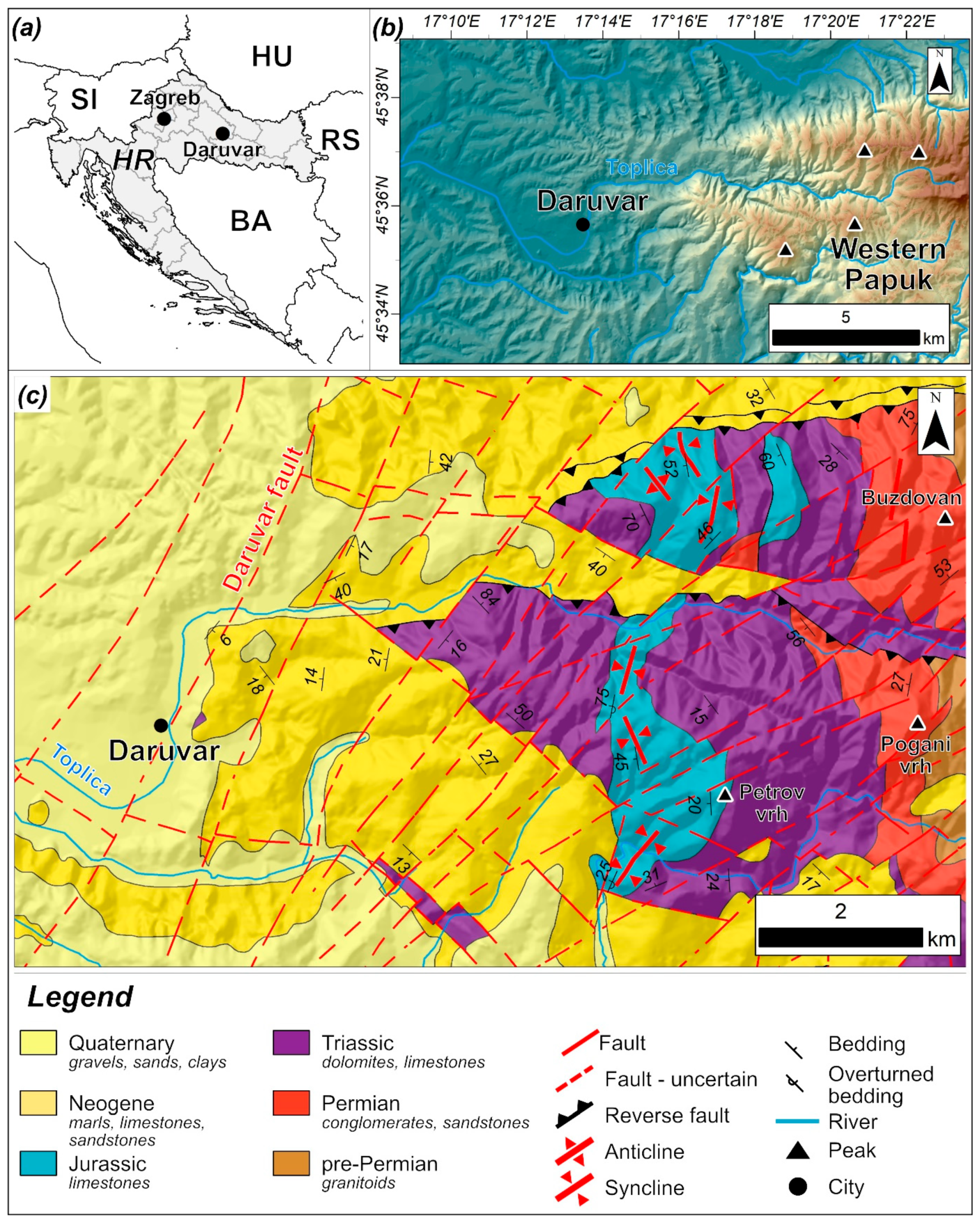
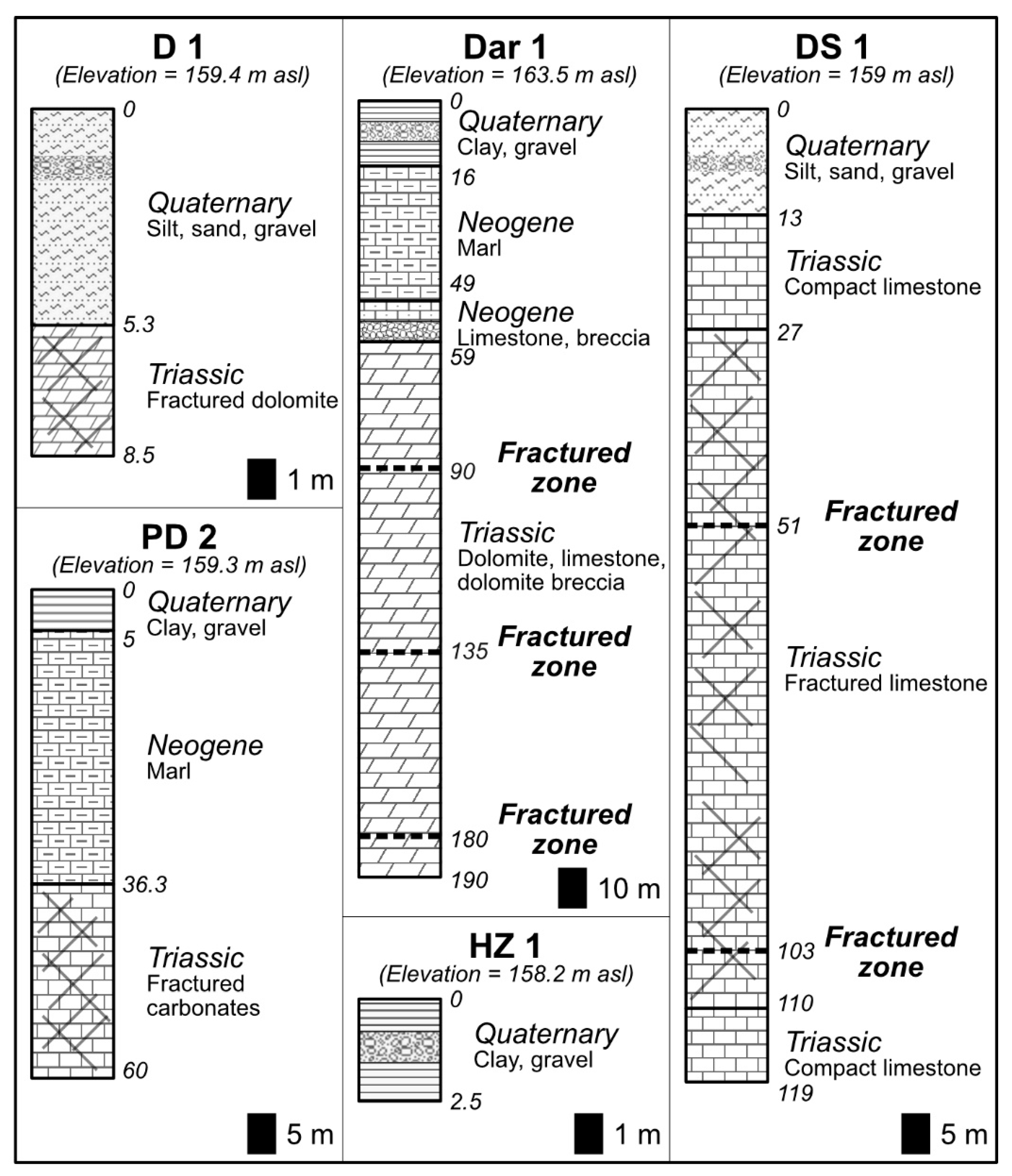
2.1. Geological and Hydrogeological Settings
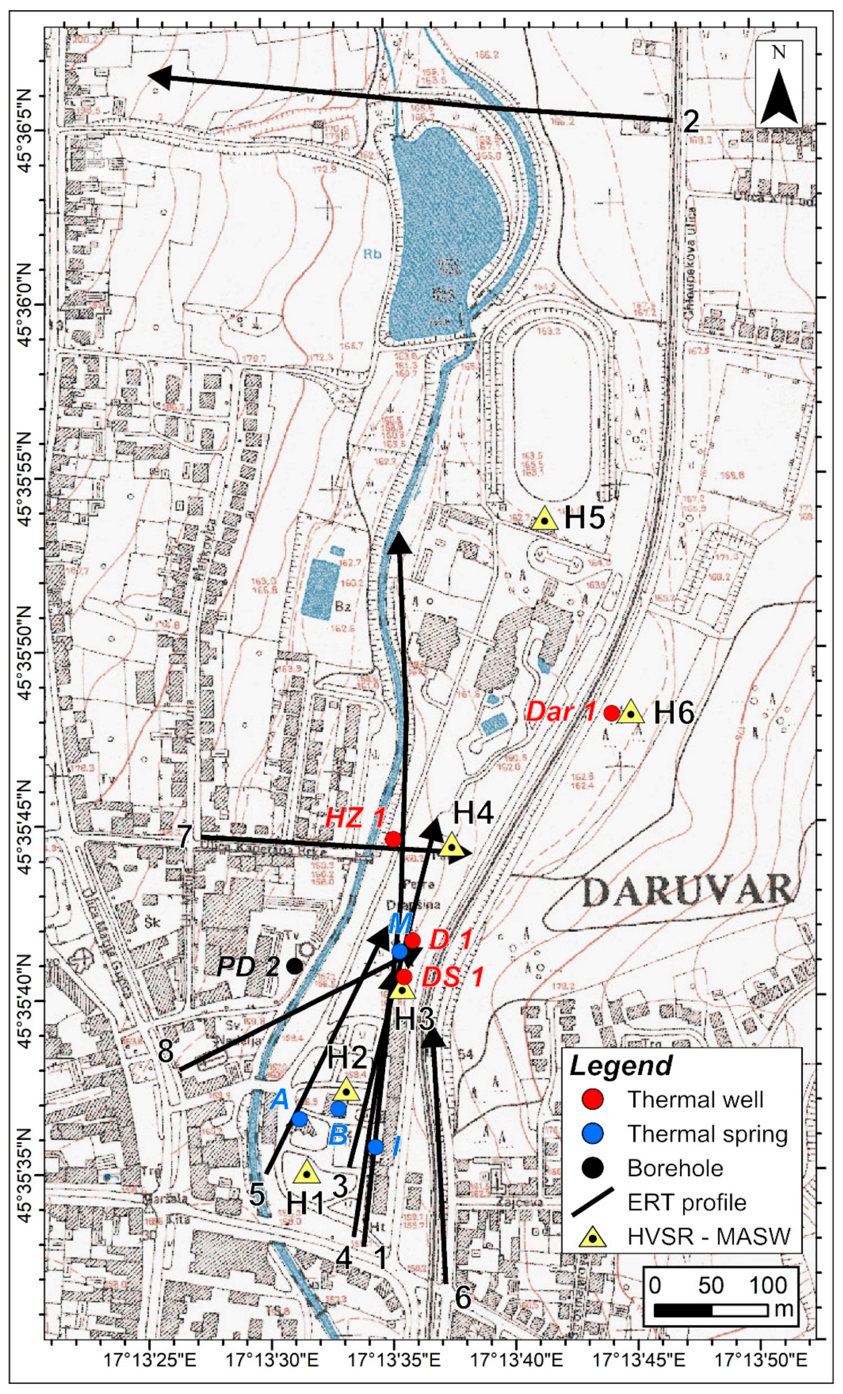
The study area (western Papuk Mt.; Figure 1b) is located at the SW margin of the PBS. The PBS is a system of basins characterized by a complex polyphase deformation history that developed parallel with the Alpine–Dinarides–Carpathian orogen. The Croatian part of the PBS [47,48,49,50] was affected by an initial E-W extensional tectonic phase during the Early to Middle Miocene that formed systems of grabens and half-grabens, i.e., regional depressions (e.g., Drava and Sava depressions; [47]). The initial extension was followed by a Middle Miocene local scale compression and a Middle to Late Miocene deepening of the basin system due to crustal thermal subsidence. Tectonic inversion and structural reactivation commenced during the Pliocene–Quaternary, which enabled the regional compression/transpression of existing structures as a result of the continuous Adria–Europe plates collision and the general N-S compression [51]. The present-day structural setting of the Papuk area is mostly affected by the last Pliocene–Quaternary deformational phase characterized by compression/transpression [52]. The N-S compression caused the reactivation of two regional dextral faults, producing a conjugated fault set composed of NW-SE dextral and NE-SW sinistral faults in their interaction zone [52]. Progressive regional transpression was accommodated by folding and uplifting of the structures along the sinistral strike-slip faults. One of those sinistral faults is the Daruvar fault (Figure 1c), which affected the local geological and structural settings of the Daruvar spring area.
Lithostratigraphic units of western Papuk Mt. (Figure 1c) can be grouped into [46]: (i) pre-Permian granitoids, (ii) Permian units consisting of well-layered conglomerates and quartz sandstones, (iii) Triassic sedimentary rock complex composed of Lower Triassic quartz sandstones and laminated shales and Middle and Upper Triassic dolomites and limestones, (iv) Jurassic laminated limestones, (v) Neogene sedimentary complex consisting of marls, limestones, and sandstones, and (vi) Quaternary alluvial and colluvial unconsolidated sediments made of an alternation of clays, sands, and gravels.
The Daruvar spring area is located on the left bank of the Toplica river in the center of Daruvar town (Figure 1c). It consists of a few thermal springs (Antunovo vrelo, Blatna kupelj, Ivanovo vrelo, and Marijina vrela springs; Figure 2) with temperatures ranging from 38 to 50 °C [44]. In addition, 109 boreholes had been drilled from 1971 to 2009 [43,53]. The most important wells are D 1, Dar 1, DS 1, and HZ 1 (8.5, 190, 119, and 2.5 m deep, respectively; Figure 2 and Figure 3) with temperatures from 22.7 to 43.5 °C [54]. Furthermore, the PD 2 exploration well (60 m deep; Figure 2 and Figure 3) was drilled to the west of the spring area on the right bank of the Toplica river [55]. Among these objects, the D 1 well and the Antunovo vrelo and Ivanovo vrelo springs are exploited for supplying the Daruvar spa and pool complexes.
The Dar 1 well (Figure 3) shows the most comprehensive stratigraphic sequence in the spring area [56]. It is composed of: (i) Quaternary unconsolidated sediments mostly made of clays, sands, and gravels, (ii) a Miocene sedimentary complex, which is constituted by marls, lithotamnian limestones, and compact breccias locally marking the unconformity at the base of Badenian [57], and (iii) a Triassic carbonate complex with dolomites, limestones, and dolomitic breccias. The Neogene–Quaternary tectonic activity in the Daruvar area was proven by the occurrence of highly fractured intervals at depths of approximately 90, 135, 180, and 190 m. In the spring area (i.e., D 1 and DS 1 wells; Figure 3), the Triassic carbonate complex is in direct contact with the alluvial deposits.
The Triassic carbonate complex represents the main thermal aquifer, with high permeability (transmissivity of 1361 m2/day; [58]) and secondary porosity resulting from the intense fracturing of the bedrock. Furthermore, thermal waters can be found in the gravel and sandy layers of the alluvial cover. The thermal water shows a predominant CaMg-HCO3 hydrochemical facies, neutral pH ranging from 6.7 to 7.5, and an electrical conductivity of approximately 600 μS/cm [54]. The hydrochemical facies and the Mg2+/Ca2+ versus Mg2+ ratio close to 0.5 [54] corroborate an interaction of the thermal waters with both limestones and dolomites. Furthermore, stable isotope composition suggests a meteoric origin of the waters.
Ref. [44] proposed a conceptual model of the DHS. The recharge area is situated in the eastern hinterland of Daruvar (i.e., western slopes of Papuk Mt.), encompassing the Mesozoic carbonate complex (Figure 1c). Mesozoic carbonates are highly permeable, enabling the deep infiltration of meteoric water. The infiltrated water reaches a depth of approximately 1 km and warms due to the increased heat flow in this part of the PBS (i.e., 80 mW/m2; [42]), resulting in a slightly high geothermal gradient. Permian clastic sedimentary units and pre-Permian crystalline rocks represent a barrier to deeper infiltration. In the area of Daruvar, the Mesozoic reservoir is tectonically brought in contact with younger Neogene rocks by the Daruvar fault. Due to the generally low permeability of the Neogene units, this contact is a lateral barrier for fluid circulation. The damage zone of the Daruvar fault increases the permeability field in the Daruvar spring area, being the main path for the rising and outflow of thermal waters. Despite its importance in the thermal water outflow, the architecture of the damage zone of the Daruvar fault is in general unknown.

2.2. Methods

2.2.1. Electrical Resistivity Tomography

Electrical resistivity tomography (ERT) is a geophysical method that is extensively applied to reconstruct the geometry of lithologies and structures in the subsurface [20,33,59]. ERT can be used to image the electrical resistivity distribution of the subsurface by injecting electrical currents and measuring electrical potentials along a profile. The resistivity generally depends on the mineralogical composition of the subsurface, its porosity, the water content, and the physical and chemical properties of the water [60]. ERT has been profitably applied in hydrogeological and structural investigations in many geothermal systems [22,23,24,61,62,63].
In this work, ERT was employed to delineate the structural and lithological properties of the Daruvar spring area. Eight profiles were acquired in 2021 and 2022 (Figure 2 and Table 1). Field measurements were conducted using the POLARES 2.0 electrical imaging system (PASI srl). This system was connected to stainless steel electrodes, which were laid out in a straight line with a constant spacing via a multi-core cable. Due to the complexity of the geological structures in the subsurface of the spring area, a Wenner–Schlumberger configuration was used since it resolves horizontal and vertical structures and has a greater depth of investigation [64]. Initially, profiles were measured at a frequency of 7.15 Hz and a maximum phase of 20° between the voltage signal and the current signal. Contact impedance value of the electrodes was checked since it can cause potential errors in the dataset [65]. The frequency was progressively lowered until the number of incorrect measurements was below 10% of the total.
The Res2DInv 4.9.3 software (https://www.aarhusgeosoftware.dk/res2dinv, accessed on 3 August 2023) was used to invert the field apparent resistivity data into 2D resistivity subsurface models using a Gauss–Newton method and a finite element solver [66,67]. The software has two different routines for creating 2D resistivity models based on the L1-norm (or blocky, robust) and the L2-norm (or smoothness-constrained least-squares) inversion methods [68]. For the collected dataset, the method based on L2 norm was used because it gives optimal results where the subsurface resistivity changes in a gradual manner. This method minimizes the sum of squares of the spatial changes in the model resistivity and the data misfit [69]. In the Daruvar spring area, materials with both relatively high and low resistivity are expected. However, the occurrence of thermal water with high electrical conductivity and the high porosity of the sediments/rocks should decrease the bulk resistivities, resulting in smooth resistivity transitions between the different formations. The inversion was terminated when the RMS was below 10%, except for profile ERT 4 for which it reached 12.4%.

2.2.2. Seismic Investigations

An integrated approach based on the passive horizontal to vertical spectral ratio (HVSR) and the active multichannel analysis of surface waves (MASW) methods was applied to map the thickness of the Quaternary cover in the Daruvar spring area. Similar methodological approaches have been used in thermal areas where recent sediments conceal the geometry of the bedrock [39,70,71,72].
The HVSR method is based on recording the vertical and horizontal components of the ambient seismic noise wavefield [73]. The seismic impedance contrast between the bedrock and the unconsolidated Quaternary sediments generates a peak in the H/V curve (i.e., ratio between the horizontal and vertical seismic ambient noise spectra) that can be used to assess the thickness of the alluvial cover. The thickness of the covering layer (h) can be calculated [73] as:
h = V s 4 f 0
with Vs being the shear-wave velocity of the sediments and f0 the peak frequency of the H/V noise spectra.
The estimation of h depends on the subsurface Vs. This parameter can be assessed using the MASW approach in order to have a site-specific distribution of Vs. The Vs profile is reconstructed by measuring the propagation velocities of surface waves in the ground [74,75]. The dispersion curve of the surface waves is calculated resulting in the 1D model of Vs variation with depth.
In this study, ambient seismic noise was recorded at 6 stations (Figure 2 and Table 2). Stations H1 to H5 were selected to perform a N-S cross section parallel to the ERT 1 profile, while H3 and H6 were located in correspondence with the DS 1 and Dar 1 wells, respectively. The three orthogonal components (one vertical and two horizontals, i.e., N-S and E-W) of the signal were recorded using a 3D land geophone with an eigenfrequency of 2 Hz and 24-bit data acquisition board. The recording time for each station was 15 min with a sampling rate of 5 ms (sampling frequency of 200 Hz). At the same site, MASW investigations were conducted through seismic profiles composed of 24 geophones (4.5 Hz) at a distance of 2 m connected to a GEA-24 seismograph (PASI srl). As the source of the seismic wave, a hammer weighing 8 kg and a steel plate were used. The center of the seismic profile was located where the HVSR measurement was conducted.
The data analysis consisted of (i) the computation of the H/V curve, (ii) the reconstruction of the Vs profile from MASW measurement, and (iii) the calculation of h at every site using Equation (1). Data processing of HVSR measurements was performed in the Geopsy 3.3.3 software (https://www.geopsy.org, accessed on 15 February 2023). For each measurement point, the Fourier amplitude spectrum of horizontal and vertical components of the ambient seismic noise was conducted. For calculating the Fourier spectrum, the Konno and Ohmachi smoothing method was used [76], then the frequency range within which the spectra are calculated was defined. Finally, the H/V ratio was calculated. When calculating and displaying the H/V spectrum, the frequency range from 0.2 to 10 Hz was used.
Processing of the MASW measurement data was conducted in the ParkSEIS 3.0 program (https://www.parkseismic.com/parkseis/, accessed on 3 August 2023). The Fourier spectral analysis was performed for each individual recording in the time domain, obtaining the dispersion curve of the S-waves. By inversion of the dispersion curve, a 1D model of the change in S-wave velocity (Vs) was calculated [75]. In the performed inversions, an input model composed of 10 layers with a thickness of 2 m was used. The iteration was stopped when the error was lower than 5%. The input model was chosen after a preliminary analysis obtaining a good vertical resolution and reaching an observation depth that would be comparable with the presumed depth of the Quaternary cover in the Daruvar spring area.

3. Results

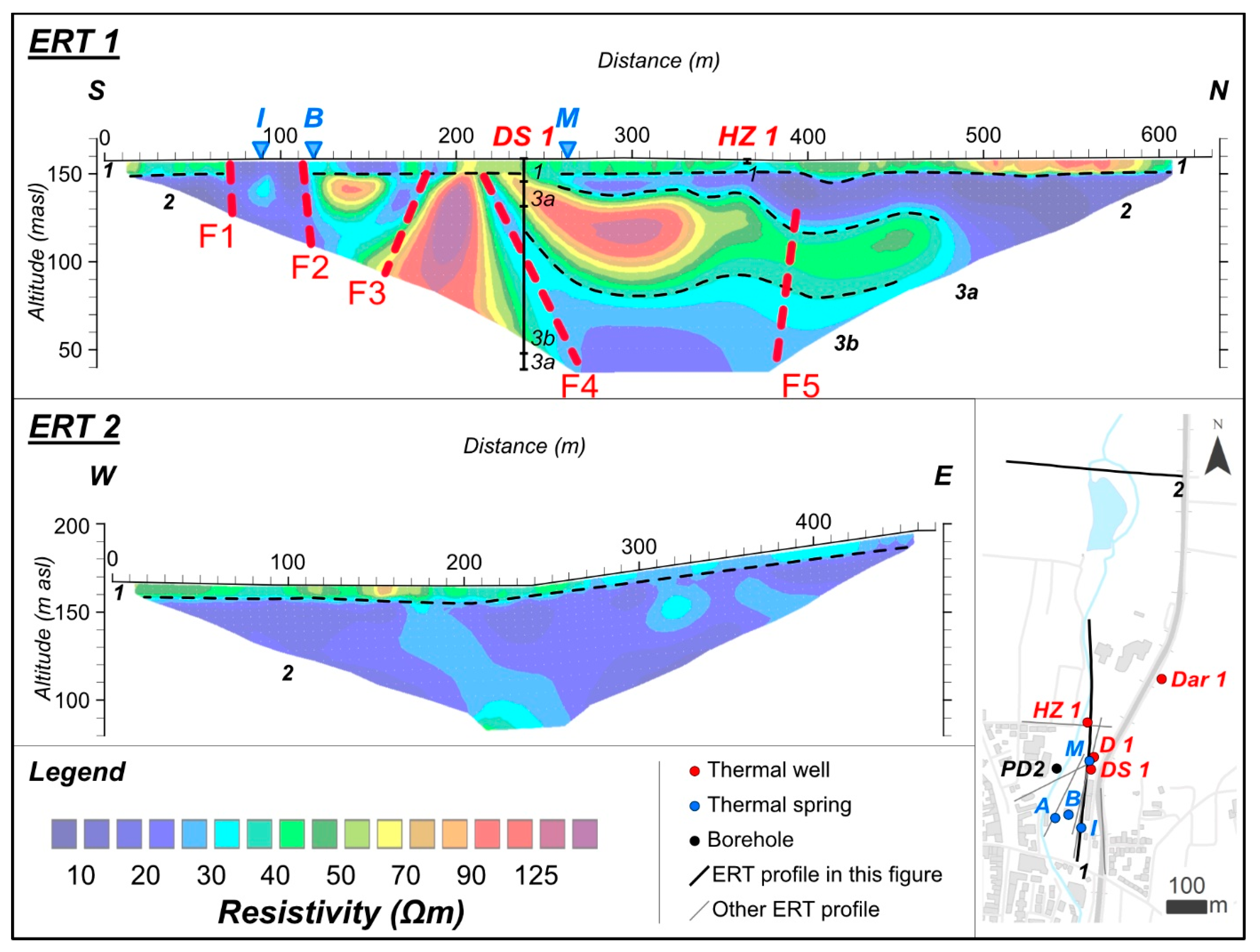
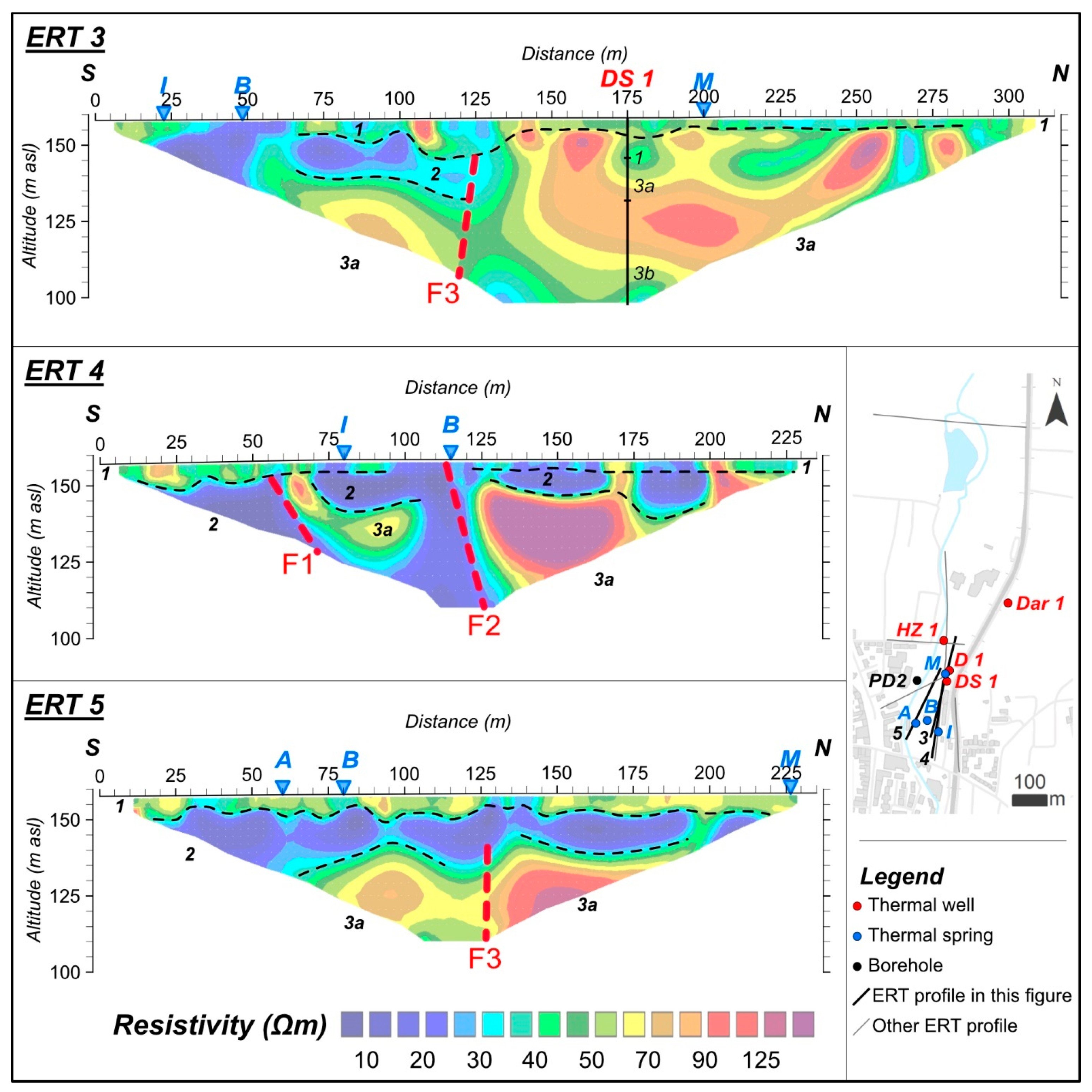
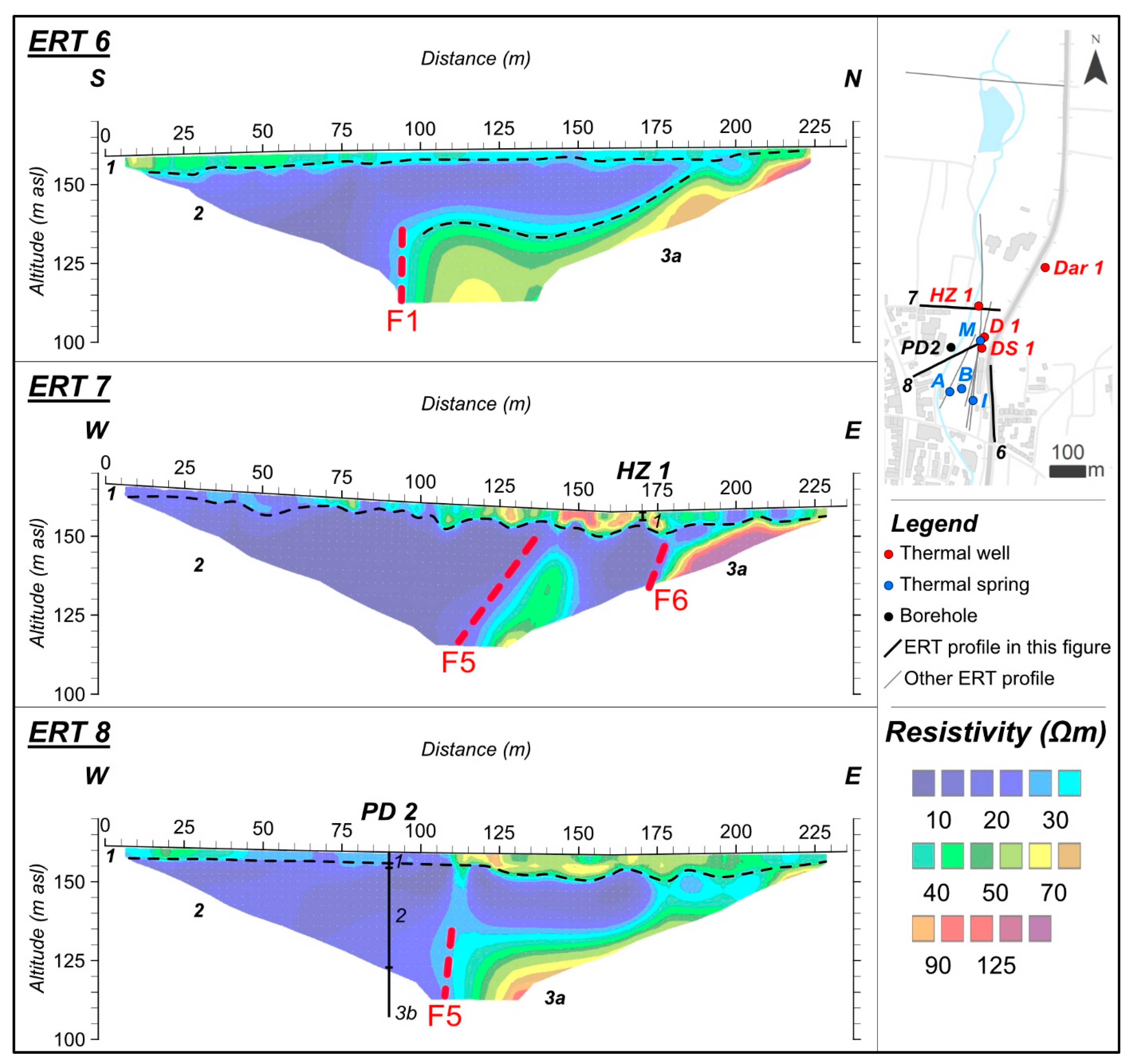
3.1. Electrical Resistivity Tomography (ERT)

The distribution of resistivity in the subsurface of the Daruvar area shows relatively low values, generally from 10 to 150 Ωm (Figure 4, Figure 5 and Figure 6).
Figure 4 shows the profiles with spacing between electrodes of 10 m providing a general overview of the spring area (i.e., ERT 1) and its surroundings (i.e., ERT 2). Data inversion resulted in an RMS error of 7% and 2.5% for ERT 1 and ERT 2, respectively.
The following layers were interpreted in ERT 1: (i) an upper domain (layer 1) with variable thickness of 5–10 m and resistivity of 30–50 Ωm, with localized anomalies of both low (<20 Ωm) and high (70–100 Ωm) resistivity, (ii) a second layer (2) with low resistivity (5–15 Ωm) showing a discontinuous geometry with a variable thickness of at least 20 m in the southern part, 5 m in the central part, and increasing up to 40 m in the northern part of the profile, (iii) a third layer (3a) with a thickness of approximately 50 m and resistivity generally ranging from 70 to 150 Ωm (and locally up to 224 Ωm) in the middle part of the profile and with a resistivity of 50–60 Ωm in the northern part, and (iv) a bottom layer (3b) characterized by resistivity values of 20–30 Ωm detected only in the central part of the profile. Additionally, several vertical low resistivity zones (10–30 Ωm) dividing the high resistivity bodies were observed (i.e., F1 to F5; Figure 4).
The layers interpreted in ERT 2 were: (i) an upper domain (layer 1) with a thickness of 5–10 m and resistivity value decreasing from W to E (40 to 20 Ωm), and (ii) a second layer (2) showing resistivity of 20–30 Ωm and reaching a thickness of approximately 80 m in the middle part of the profile.
Figure 5 shows the profiles investigating the spring area conducted using a spacing between electrodes of 5 m. Data inversion resulted in an RMS error of 4.1%, 12.4%, and 5.6% for ERT 3, ERT 4, and ERT 5, respectively.
Three domains can be distinguished in the profile ERT 3: (i) an upper domain (layer 1) which has a variable thickness of 5–10 m and is characterized by resistivity values of 30–50 Ωm with small scale resistivity anomalies, (ii) a second domain (layer 2), visible only in the southern part of profile, with low resistivity of 10–30 Ωm, and (iii) a third domain (layer 3a) located at a depth higher than 20 m in the southern part of the profile and with resistivity values of 40–70 Ωm, and located at a depth higher than 5 m in the central and northern part of the profile having resistivity generally between 50 and 100 Ωm (locally up to 160 Ωm). Within layer 3a, a lateral decrease of resistivity is observed at the distance between 125–135 m showing a prominent sub-vertical geometry and resistivity values of 30–40 Ωm (F3). Furthermore, a low resistivity area (10–20 Ωm) is depicted in the southern part of the profile in correspondence with the Ivanovo vrelo and Blatna kupelj springs.
In the profile ERT 4, the interpreted layers are: (i) an upper domain (layer 1) with a maximum thickness of 5 m and a variable resistivity of 20–40 Ωm, (ii) a second layer (2) with a resistivity of 10–20 Ωm and a thickness higher than 15 m in the southern part and from 5 to 15 m in the central and northern part of the profile, and (iii) a bottom domain (layer 3a) divided into two zones at 60 to 100 m and 125 to 175 m with resistivity values of 40–50 Ωm and >100 Ωm (maximum resistivity of 345 Ωm), respectively. These two zones are divided by a sharp lateral decrease of resistivity with values 10–20 Ωm (F2).
Three domains can be distinguished in the profile ERT 5: (i) an upper domain (layer 1) which has a thickness of approximately 5 m and resistivity values of 40–60 Ωm and small scale resistivity anomalies, (ii) a second domain (layer 2) showing good lateral continuity, a thickness of approximately 15 m, and resistivity of 10–20 Ωm, and (iii) a third domain (layer 3a) divided into two zones at 80 to 110 m and 130 to 180 m with resistivity values of approximately 70 and >90 Ωm (maximum resistivity of 150 Ωm), respectively. The two zones are divided by a vertical body with lower resistivity values of 50–60 Ωm (F3).
Figure 6 shows the profiles with spacing between electrodes of 5 m providing an overview of the north-western (i.e., ERT 7 and ERT 8) and south-eastern parts (i.e., ERT 6) of the spring area. Data inversion resulted in an RMS error of 3.5%, 6.5%, and 2.9% for ERT 6, ERT 7, and ERT 8, respectively.
The following layers are interpreted in ERT 6: (i) an upper domain (layer 1) with a thickness of 5 m and a resistivity of 30–40 Ωm, (ii) a second layer (2) with low resistivity (<20 Ωm) and a decreasing thickness from at least 30 m in the southern part to 5 m in the northern part of the profile, and (iii) a third layer (3a) with a thickness of at least 25 m in the middle part of the profile and resistivity generally ranging from 40 to 60 Ωm (locally up to 200 Ωm). A sharp lateral transition between layers 2 and 3a is observed (F1).
Three domains can be distinguished in the profile ERT 7: (i) an upper domain (layer 1), which has a thickness of 5 m and is characterized by resistivity of 20–40 Ωm, except for a high resistivity anomaly (90–110 Ωm) at 145–175 m, (ii) a second domain (layer 2) observed in the western and central part of the section with resistivity <10 Ωm and a thickness of at least 45 m, and (iii) a third domain (layer 3a) in the eastern part of the profile characterized by resistivity from 50 to 100 Ωm in the upper part and from 200 to 300 Ωm in the deeper part. The layer 3a shows a sharp transition to a very low resistivity body (<10 Ωm) towards the W (F6). Moving westward, the resistivity slightly increases (30–40 Ωm), followed by a sharp resistivity drop and the transition to layer 2 (F5).
Three layers based on the resistivity distribution are observed in ERT 8: (i) an upper domain (layer 1), which has a thickness of approximately 5 m and is characterized by low resistivity of 20–30 Ωm until 115 m, followed by slightly higher resistivity values (40–60 Ωm), (ii) a second domain (layer 2), which has a resistivity of 10–30 Ωm and a variable thickness of at least 45 m in the western part, approximately 25 m from 110 m to 170 m, and 10 m in the eastern part of the profile, and (iii) a third layer (3a) at a depth of 30 m in the central part of the profile with resistivity values of generally 40–70 Ωm and reaching values of approximately 100 Ωm in the deeper part of the layer. A sharp lateral transition between layers 2 and 3a is observed (F5).

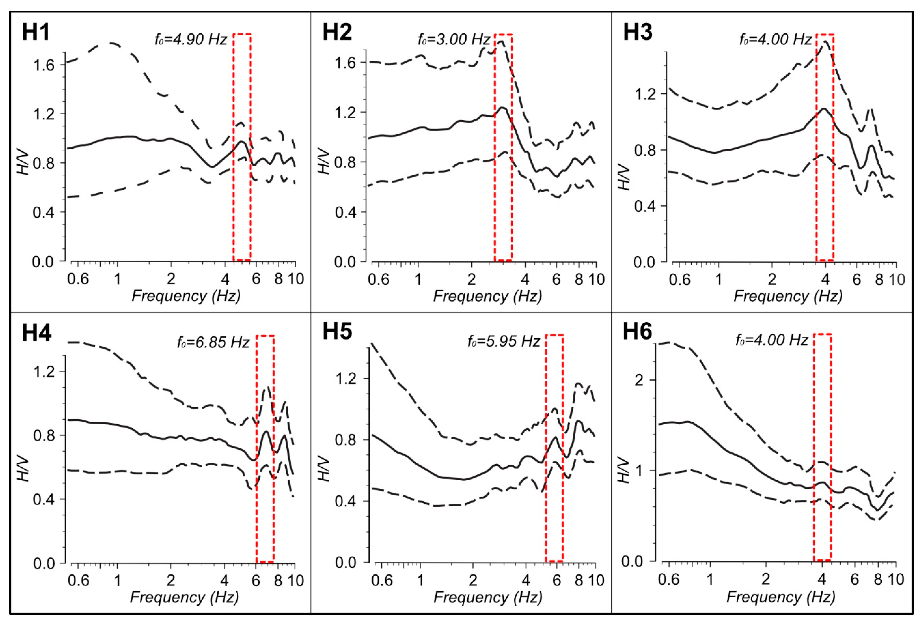
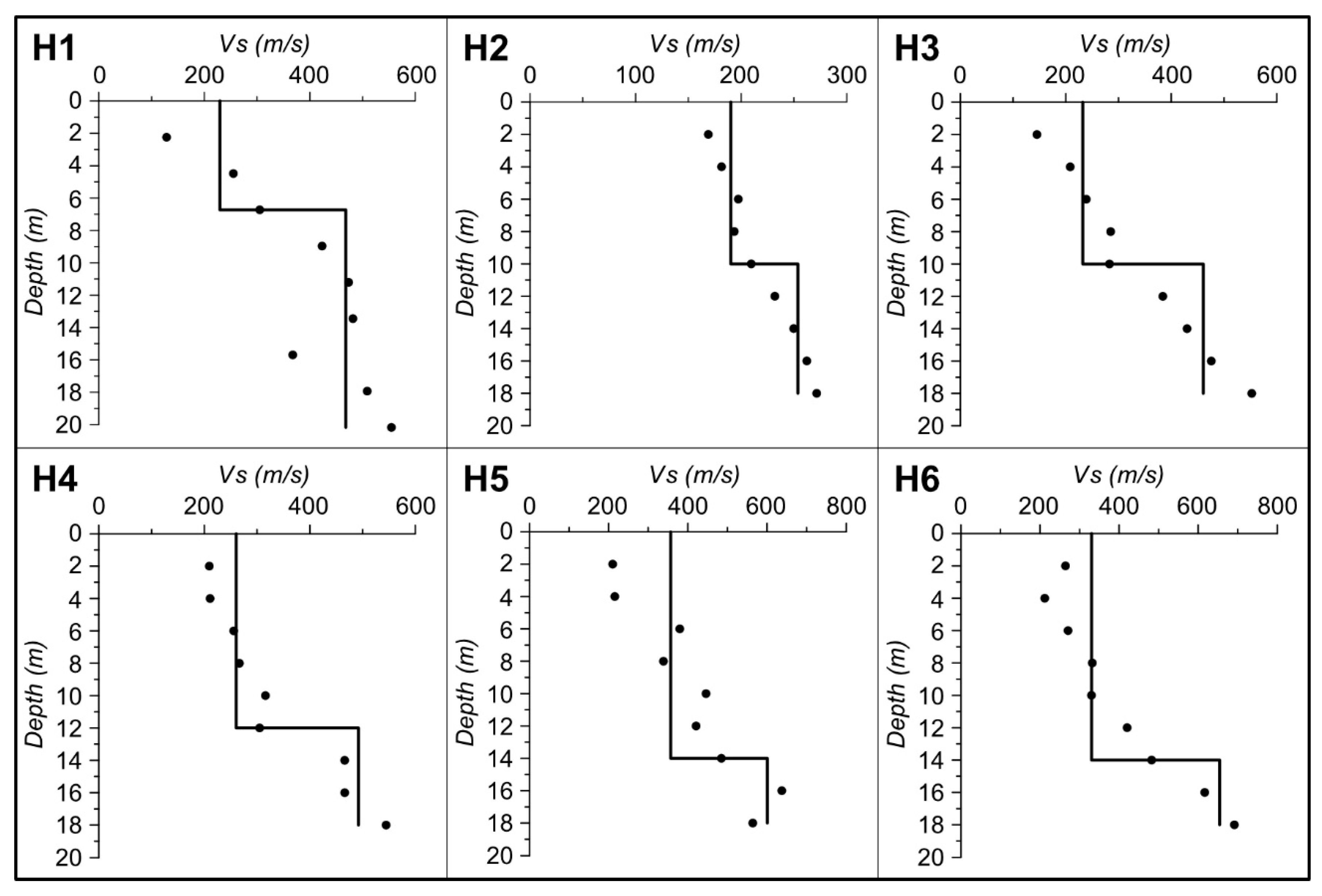
3.2. Seismic Investigations

H/V spectral ratio method was applied to the six microtremor measurements (Figure 2 and Table 2) conducted in the Daruvar spring area. The results are shown in Figure 7. The interpreted H/V curves present f0 peaks with variable shapes, from sharp to smooth, indicating a heterogenous seismic response in the subsurface. Generally, the measurements show sharp peaks in the H/V curve, except for H6 towards the east. The f0 and amplitude of the peaks are reported in Table 3.
Furthermore, a reconstruction of the vertical variation in S-wave velocity (Vs) was conducted through the measurement of the ambient seismic noise using the MASW approach. The reached investigation depth was 20 m, and the Vs distributions at the different locations are shown in Figure 8. Vs values generally range from approximately 125 m/s to 690 m/s (black dots in Figure 8).
The observed Vs were grouped based on the Vs values (black lines in Figure 8). Two seismic units can be distinguished. The thickness of the first seismic unit varies from 6 to 14 m, showing Vs from 190 to 356 m/s. Vs values in the second seismic unit range from 253 m/s to 654 m/s. It should be noted that H2 shows the lowest Vs values for both the first and the second seismic units.
The H/V frequency and the Vs of the first layer were used to estimate the thickness of the sedimentary cover, corresponding to the Quaternary alluvial cover, using Equation (1). The results are shown in Table 3.

4. Discussion

Reconstruction of the geological setting of a thermal system is one of the steps necessary for assessing the potential of a geothermal resource. Geophysical investigations have been profitably used to address this topic since their results can be used to indirectly reconstruct the geometry of the reservoir and of the fault systems driving the fluid circulation [19,22,23,24,39,61,62,63,71,72]. These methods are particularly applicable in areas where the geological data are limited to a few stratigraphic logs or where the alluvial cover conceals the subsurface structure.
In this work, an integrated geophysical approach based on electrical resistivity tomography (ERT) and both active and passive seismic (i.e., MASW and HVSR) methods was applied to construct a 3D model of the subsurface in the Daruvar spring area (Figure 2). The outflow of thermal waters in the study area is enhanced by the high permeability of the carbonate reservoir, resulting in thermal springs with water temperatures of 38–50 °C [44]. Although it was argued that the increased permeability field is connected with faults and their damage zones, their occurrence has never been proven.
The ERT profiles in the Daruvar area (Figure 2) showed heterogenous vertical and horizontal resistivity distributions (Figure 4, Figure 5 and Figure 6). Four layers were recognized. A first, near-surface layer (layer 1) with resistivity values ranging from 30 to 50 Ωm was observed in all profiles (Figure 4, Figure 5 and Figure 6). This domain contains zones with low (<20 Ωm) and high (generally 70–100 Ωm) resistivity values, and its thickness varies from 5 to 10 m. The second layer (layer 2) showed discontinuous geometry with thickness variations from 20 to 40 m and a uniform resistivity ranging from 5 to 25 Ωm (Figure 4, Figure 5 and Figure 6). The third layer (3a) had a maximum thickness of 50 m and resistivities ranging from 70 to 150 Ωm. A bottom layer (3b) was detected only in the central part of the longest profile (ERT 1; Figure 4) and it was characterized by resistivity values of 20–30 Ωm.
The lithologies of the observed layers were assessed considering the stratigraphic logs of the wells in the Daruvar thermal spring area (Figure 2 and Figure 3).
Layer (1) was interpreted as the Quaternary alluvial cover composed of interchanging clays, sands, and gravels. Clay sediments generally show low resistivities (10–100 Ωm; [18]), while sands and gravels have higher resistivity (>200 Ωm; [60]). Considering the wide range of resistivity in granular materials, relatively low resistivity values were observed in layer 1. However, the occurrence of water in the pore spaces and its chemical composition and temperature could diminish the bulk electrical resistivity of the material. Reports of boreholes highlighted that the sandy layers of the alluvial cover host both fresh waters infiltrating from the Toplica river and thermal waters with moderate mineralization. Locally, the water content in the pore spaces could be lower, causing a local increase in the resistivity as shown by the ERT profiles.
Layer (2) was interpreted as the Neogene sedimentary complex of western Papuk mostly consisting of marls and locally bioclastic limestones in the lower part. Marls generally show resistivities in the range of 50–100 Ωm [34]. Similar to the Quaternary deposits, Neogene marls in the Daruvar area could be saturated with thermal or cold waters, causing the observed low resistivity values (5–25 Ωm).
Layer (3) was interpreted as the Triassic sedimentary rocks complex composed of dolomites and limestones. Based on the difference in the resistivity distribution, this layer was divided into a “more compact” and a “more fractured” part (i.e., layer 3a and 3b, respectively) with higher (70–150 Ωm) and lower (20–30 Ωm) resistivity values, respectively. The resistivity of carbonate rocks is generally higher than 800 Ωm [18]. On the other hand, the resistivities measured in layer 3 are much lower for both the compact and fractured parts. In order to estimate their bulk resistivity, the generalized version of the Archie’s law [77,78,79] was used:
ρ = a ϕ m S n ρ w
with ρ and ρw being the bulk and water resistivity, respectively, ϕ the porosity of the material, S the water saturation, and a, m, and n empirical parameters. Layer 3 was considered fully saturated (i.e., S = 1) by the Daruvar thermal waters. The ρw was calculated from the average electrical conductivity of the thermal water measured in the Antunovo vrelo spring (i.e., 578 μS/cm; [54]). The porosity was obtained from the well logging conducted in the Dar 1 well [56]. The average porosity value (7%) was considered representative of the compact carbonates since it permits the inclusion of small scale fractures that could not be highlighted during the well drilling but could contain thermal waters. The value at the 90th percentile of the porosity distribution (17%) was considered representative of the fractured portion since it permits the inclusion of both small- and large-scale fractures. The empirical parameters a and m were both set as equal to 1. These values are generally considered appropriate for a preliminary assessment of the resistivity in fractured carbonates [78,79,80,81]. The resulting ρ for the compact and the fractured parts of layer 3 (i.e., 3a and 3b, respectively) were 220 and 100 Ωm, respectively. These values are in the upper range of the observed values. However, it could be argued that the porosities measured through the well logging are representative of a rock volume smaller than the volume investigated with ERT. Increasing the representative elementary volume would increase the porosity [82], resulting in a decrease of the bulk resistivity.
Besides vertical variations in the resistivity distribution, lateral variations were observed (F1 to F5 in Figure 4, Figure 5 and Figure 6). They were generally marked by low resistivity anomalies (up to 20 Ωm) within higher resistivity bodies (i.e., F4 in ERT 1; Figure 4) or by a sharp transition in the resistivity distribution (i.e., F5 in ERT 6 and ERT 7; Figure 6). These lateral variations were interpreted as caused by the occurrence of faults/fractures and associated damage zones. The high secondary porosity of the fault damage zone and the occurrence of thermal waters decrease the bulk resistivity of the rock mass, resulting in the observed anomalies. Archie’s law (Equation (2)) was used to assess the bulk resistivity of the fault damage zone. The highest porosity value measured during the Dar 1 well logging (41%) was considered representative since it could reflect a highly fractured rock mass with open fractures that is typical of a fault damage zone. Other parameters were kept constant. The resulting ρ was 40 Ωm, very similar to the observed values.
The results of ERT profiles were complemented by the results obtained from active and passive seismic methods. These methods were used to define the thickness of the Quaternary cover through the Nakamura approach [73] (Equation (1)). The reliability of the method was verified by comparing the results with the stratigraphic logs at the same locations. A thickness of 14.5 and 20.6 m was calculated at H3 and H6 (Table 3), respectively, roughly corresponding to the alluvial cover thickness in DS 1 and Dar 1 (Figure 3), respectively. In general, the estimated sedimentary thickness increased from a minimum value of 9.5 m in the central part of the study area (H4; Table 3 and Figure 2) to 11.7 m and 15 m towards south and north (i.e., H1 and H5, respectively; Table 3 and Figure 2). The results obtained by seismic investigations are comparable with the thickness of layer 1 in ERT 1 profile corroborating the results of the electrical resistivity tomography investigations.
Results of the integrated geophysical approach (i.e., ERT, MASW, and HVSR) and data from the stratigraphic logs of the wells were used to construct the 3D geological model of the thermal spring area in Daruvar. The Petroleum Experts Move 2019.1 (https://www.petex.com/products/move-suite/move/, accessed on 13 May 2023) software package was used since it allows integrating 1D and 2D data for a 3D visualization and analysis. Stratigraphic horizons, corresponding to the base of principal lithostratigraphic units/formations, were reconstructed as planes using the inverse distance weight algorithm based on the stratigraphic limits in the ERT profiles and the stratigraphic logs. Fault surfaces were constructed as planes with the spline curves algorithm based on the fault lines interpreted on the ERT sections.
The constructed 3D geological model (Figure 9) is oriented S-N, covering an area of approximately 400 × 600 m and reaching a depth of approximately 120 m, which corresponds to the maximum investigation depth of the ERT profiles. The ERT 2 profile was not used during the construction of the 3D model, since it is located far from other sections and it would result in significant uncertainty in the model.
Three stratigraphic units and four faults were modeled (Figure 9).
The first unit corresponds to the Quaternary alluvial cover with a variable thickness between 10 and 15 m. The second unit corresponds to the Neogene sedimentary complex. Its thickness is a few meters in the central part of the Daruvar spring area and increases toward the S and the N. It reaches a maximum of 40 and 30 m in the SW and SE corners, respectively, while it is up to 100 and 50 m in the NW and NE corners, respectively. It should be noted that the highest modeled thickness has a high uncertainty since data are not available in this part of the model. The third unit is composed of the Triassic carbonate complex that constitutes the main thermal reservoir. Its geometry has been partially reproduced since its bottom was arbitrarily placed at a depth of 120 m, corresponding to the maximum depth investigated with the ERT profiles. However, neither the profiles nor the wells reached the bottom of the reservoir unit, and its real thickness in the spring area is still debatable. In the central part of the study area, the Triassic complex is in direct contact with the Quaternary unit (i.e., ERT 1 and 3; Figure 4 and Figure 5).
The modeled faults were F1, F2, F3, and F5 (Figure 9). The fault traces F4 (ERT 1; Figure 4) and F6 (ERT 7; Figure 6) were not modeled since they were depicted only in one profile. The fault F1 dips at a high angle toward NNE showing a length of 300 m in plain view. The dip direction varies from approximately 10°N in the eastern part to 40°N in the western part toward the contact with F5. Similarly, the dip decreases westward from subvertical to approximately 70° at the contact with F5. The fault F2 dips at high angle (>80°) toward ENE (dip direction = 60–70°N) with a length of 130 m in plain view. The fault F3 dips at a high angle (80°) toward the S (dip direction = 180°N) with a length of 250 m in plain view. Fault F5 is the longest in the modeled area, extending within the whole modeling domain. The fault generally dips toward the W (dip direction = 280°N) at different angles. The dip varies from 85° in the southern part of the modeling domain to 65° toward the N.
The faults show a minor vertical throw, and only F5 shows a throw up to 15 m (ERT 8; Figure 6). Since shallow geophysical methods were employed in this work, the data on the vertical extent of the faults are limited and deeper data should be acquired in the future for a detailed kinematic analysis. Similarly, it is not possible to determine the horizontal movement.
F1 and F3 can be interpreted as E-W trending, high angle, antithetic faults, while F2 could represent a splay fault within their interaction zone. F5 borders westward the interaction zone and could be interpreted as a fault parallel to the regional, NE-SW trending, Daruvar fault, or it could correspond to its shallower part. Here, for a detailed interpretation addressing the relation between F5 and the Daruvar fault, a regional reconstruction should be performed.
The main outflow of the Daruvar thermal waters, represented by the Antunovo vrelo, Blatna kupelj, and Ivanovo vrelo springs (Figure 2 and Figure 9), occurs within this interaction zone of the observed/mapped faults. The faults F1 and F5 border the interaction zone toward the S and the W, and accommodated the uplifting of the main thermal reservoir (i.e., Triassic carbonates) to shallow depths. Interaction zones between faults are preferential locations for the occurrence of thermal springs, and in general geothermal resources, since the kinematic transfer between the faults increases the rock fracturing and the permeability field [11,12]. This result improves the available conceptual model of the DHS, proving that the occurrence of an interaction zone between faults locally increases the permeability field of the aquifer, favoring the upwelling of the Daruvar thermal waters, and resulting in the observed thermal springs. A similar structure could occur at a larger scale, justifying the high transmissivity of the thermal aquifer calculated through the pumping test conducted in the Dar 1 well [56,58]. Furthermore, the faults F1 and F5 border westward and southward the Daruvar spring area, laterally juxtaposing the high permeable thermal aquifer with low permeable units (i.e., Neogene marls). The lateral contrast in the permeability could foster and localize the upwelling of the thermal waters.

5. Conclusions

The sustainable exploitation of a geothermal resource for its long-term utilization is related to both the water demand and the geological and hydrogeological characteristics of the geothermal field. Detailed geological modeling is a key factor for estimating the potential of a geothermal resource.
This research focused on the reconstruction of the geological and structural settings of the Daruvar thermal spring area using different geophysical methods. Their joint interpretation completed with the stratigraphic logs of exploitation wells and boreholes allowed the determination of the vertical and horizontal distributions of lithological units and proved the occurrence of faults deforming the bedrock in the Daruvar area. The data were used as the input for a 3D model that favored a better visualization and analysis of the results, improving the conceptual model of the Daruvar hydrothermal system. In particular, it was proved that an interaction zone between faults deforms the bedrock, increasing the fracturing and the permeability field. These conditions are favorable for the upwelling of thermal waters and for the formation of thermal springs as depicted in several geothermal fields worldwide.
This paper fosters the knowledge about thermal systems hosted in carbonate complexes that are typical of northern Croatia and the Pannonian basin in general. It proves that a cost-effective geophysical approach could be used to investigate shallow geothermal systems. Furthermore, 3D geological modeling could be profitably used to improve the conceptual model of the system, providing insights on the connected geothermal resource and its sustainable utilization. In particular, the constructed 3D local model of the Daruvar spring area could be used in a regional- to local-scale reconstruction of the Daruvar hydrothermal system. Such multi-scale models are crucial for assessing the hydrogeological and thermal processes driving the development of a thermal system and can provide useful insights on the renewability of the geothermal resource and the sustainability of its utilization.

Author Contributions

Conceptualization and methodology, B.M., I.K., M.P. (Marco Pola), M.B. and S.B.; data collection by all authors; data curation, I.K. and M.P. (Marco Pola); software and formal analysis, I.K., I.P., M.P. (Marco Pola) and B.P.; writing—original draft preparation, M.P. (Marco Pola); writing—review and editing by all authors; visualization, I.K., B.M. and M.P. (Marco Pola); supervision, S.B.; research design and funding acquisition, S.B.; project administration, M.P. (Mirja Pavić) and S.B. All authors have read and agreed to the published version of the manuscript.

Funding

This research was funded by the HyTheC project of the Croatian Science Foundation (HRZZ), grant number UIP-2019-04-1218.

Institutional Review Board Statement

Not applicable.

Informed Consent Statement

Not applicable.

Data Availability Statement

Data available on request from the authors.

Acknowledgments

The authors would like to thank the colleagues H. Burić, T. Novosel, M. Mileusnić, N. Stanić, and M. Patekar for the support during the geophysical campaigns, and Daruvarske toplice–Special Hospital for Medical Rehabilitation and Pivovara Daruvar d.o.o. for logistic help on-site and sharing of existing materials.

Conflicts of Interest

The authors declare no conflict of interest.

References

  1. EU CORDIS; European Climate Infrastructure and Environment Executive Agency (CINEA). CORDIS Results Pack on Geothermal Energy—Supporting the Development of Europe’s Geothermal Energy Sector; Publications Office of the European Union: Luxembourg, 2022. [Google Scholar]
  2. Fetting, C. The European Green Deal; ESDN Report; ESDN Office: Vienna, Austria, 2020. [Google Scholar]
  3. Moeck, I.S. Catalog of Geothermal Play Types Based on Geologic Controls. Renew. Sustain. Energy Rev. 2014, 37, 867–882. [Google Scholar] [CrossRef] [Green Version]
  4. Moeck, I.; Hinz, N.; Faulds, J.; Bell, J.; Kell-Hills, A.; Louie, J. 3D Geological Mapping as a New Method in Geothermal Exploration: A Case Study from Central Nevada. GRC Trans. 2010, 34, 807–812. [Google Scholar]
  5. Pola, M.; Cacace, M.; Fabbri, P.; Piccinini, L.; Zampieri, D.; Torresan, F. Fault Control on a Thermal Anomaly: Conceptual and Numerical Modeling of a Low-Temperature Geothermal System in the Southern Alps Foreland Basin (NE Italy). J. Geophys. Res. Solid Earth 2020, 125, e2019JB017394. [Google Scholar] [CrossRef]
  6. Siler, D.L.; Faulds, J.E.; Hinz, N.H.; Dering, G.M.; Edwards, J.H.; Mayhew, B. Three-Dimensional Geologic Mapping to Assess Geothermal Potential: Examples from Nevada and Oregon. Geotherm. Energy 2019, 7, 2. [Google Scholar] [CrossRef] [Green Version]
  7. Torresan, F.; Piccinini, L.; Cacace, M.; Pola, M.; Zampieri, D.; Fabbri, P. Numerical Modeling as a Tool for Evaluating the Renewability of Geothermal Resources: The Case Study of the Euganean Geothermal System (NE Italy). Environ. Geochem. Health 2022, 44, 2135–2162. [Google Scholar] [CrossRef]
  8. Maitra, A.; Singh, A.; Keesari, T.; Sharma, S.P.; Gupta, S. Elevated Equilibrium Geotherm in Stable Continental Shield: Evidence From Integrated Structural, Hydrological, and Electromagnetic Studies on Nonvolcanic Hot Springs in the Eastern Ghats Belt, India. J. Geophys. Res. Solid Earth 2020, 125, e2019JB017747. [Google Scholar] [CrossRef]
  9. Fulignati, P.; Marianelli, P.; Sbrana, A.; Ciani, V. 3D Geothermal Modelling of the Mount Amiata Hydrothermal System in Italy. Energies 2014, 7, 7434–7453. [Google Scholar] [CrossRef] [Green Version]
  10. Torresan, F.; Piccinini, L.; Pola, M.; Zampieri, D.; Fabbri, P. 3D Hydrogeological Reconstruction of the Fault-Controlled Euganean Geothermal System (NE Italy). Eng. Geol. 2020, 274, 105740. [Google Scholar] [CrossRef]
  11. Faulds, J.E.; Hinz, N.H.; Dering, G.M.; Siler, D.L. The Hybrid Model—The Most Accommodating Structural Setting for Geothermal Power Generation in the Great Basin, Western USA. Trans.-Geotherm. Resour. Counc. 2013, 37, 3–10. [Google Scholar]
  12. Curewitz, D.; Karson, J.A. Structural Settings of Hydrothermal Outflow: Fracture Permeability Maintained by Fault Propagation and Interaction. J. Volcanol. Geotherm. Res. 1997, 79, 149–168. [Google Scholar] [CrossRef]
  13. Cacace, M.; Blöcher, G.; Watanabe, N.; Moeck, I.; Börsing, N.; Scheck-Wenderoth, M.; Kolditz, O.; Huenges, E. Modelling of Fractured Carbonate Reservoirs: Outline of a Novel Technique via a Case Study from the Molasse Basin, Southern Bavaria, Germany. Environ. Earth Sci. 2013, 70, 3585–3602. [Google Scholar] [CrossRef]
  14. Pola, M.; Gandin, A.; Tuccimei, P.; Soligo, M.; Deiana, R.; Fabbri, P.; Zampieri, D. A Multidisciplinary Approach to Understanding Carbonate Deposition under Tectonically Controlled Hydrothermal Circulation: A Case Study from a Recent Travertine Mound in the Euganean Hydrothermal System, Northern Italy. Sedimentology 2014, 61, 172–199. [Google Scholar] [CrossRef]
  15. Faulkner, D.R.; Jackson, C.A.L.; Lunn, R.J.; Schlische, R.W.; Shipton, Z.K.; Wibberley, C.A.J.; Withjack, M.O. A Review of Recent Developments Concerning the Structure, Mechanics and Fluid Flow Properties of Fault Zones. J. Struct. Geol. 2010, 32, 1557–1575. [Google Scholar] [CrossRef]
  16. Caine, J.S.; Evans, J.P.; Forster, C.B. Fault Zone Architecture and Permeability Structure. Geology 1996, 24, 1025–1028. [Google Scholar] [CrossRef]
  17. Bense, V.F.; Gleeson, T.; Loveless, S.E.; Bour, O.; Scibek, J. Fault Zone Hydrogeology. Earth-Sci. Rev. 2013, 127, 171–192. [Google Scholar] [CrossRef]
  18. Bruhn, D.; Manzella, A.; Vuataz, F.; Faulds, J.; Moeck, I.; Erbas, K. Exploration Methods. In Geothermal Energy Systems; Wiley-VCH Verlag GmbH & Co. KGaA: Weinheim, Germany, 2010; pp. 37–112. ISBN 9783527408313. [Google Scholar]
  19. Singh, A.; Sharma, S.P. Identification of Different Geologic Units Using Fuzzy Constrained Resistivity Tomography. J. Appl. Geophys. 2018, 148, 127–138. [Google Scholar] [CrossRef]
  20. Chandra, P.C. Groundwater Geophysics in Hard Rock; CRC Press: Boca Raton, FL, USA, 2015; ISBN 9780429062605. [Google Scholar]
  21. Yáñez, G.; Perez-Estay, N.; Araya-Vargas, J.; Sanhueza, J.; Figueroa, R.; Maringue, J.; Rojas, T. Shallow Anatomy of the San Ramón Fault (Chile) Constrained by Geophysical Methods: Implications for Its Role in the Andean Deformation. Tectonics 2020, 39, 2020TC006294. [Google Scholar] [CrossRef]
  22. Lévy, L.; Maurya, P.K.; Byrdina, S.; Vandemeulebrouck, J.; Sigmundsson, F.; Árnason, K.; Ricci, T.; Deldicque, D.; Roger, M.; Gibert, B.; et al. Electrical Resistivity Tomography and Time-Domain Induced Polarization Field Investigations of Geothermal Areas at Krafla, Iceland: Comparison to Borehole and Laboratory Frequency-Domain Electrical Observations. Geophys. J. Int. 2019, 218, 1469–1489. [Google Scholar] [CrossRef] [Green Version]
  23. Pérez-Estay, N.; Molina-Piernas, E.; Roquer, T.; Aravena, D.; Araya Vargas, J.; Morata, D.; Arancibia, G.; Valdenegro, P.; García, K.; Elizalde, D. Shallow Anatomy of Hydrothermal Systems Controlled by the Liquiñe-Ofqui Fault System and the Andean Transverse Faults: Geophysical Imaging of Fluid Pathways and Practical Implications for Geothermal Exploration. Geothermics 2022, 104, 102435. [Google Scholar] [CrossRef]
  24. Richards, K.; Revil, A.; Jardani, A.; Henderson, F.; Batzle, M.; Haas, A. Pattern of Shallow Ground Water Flow at Mount Princeton Hot Springs, Colorado, Using Geoelectrical Methods. J. Volcanol. Geotherm. Res. 2010, 198, 217–232. [Google Scholar] [CrossRef]
  25. Di Napoli, R.; Martorana, R.; Orsi, G.; Aiuppa, A.; Camarda, M.; De Gregorio, S.; Gagliano Candela, E.; Luzio, D.; Messina, N.; Pecoraino, G.; et al. The Structure of a Hydrothermal System from an Integrated Geochemical, Geophysical, and Geological Approach: The Ischia Island Case Study. Geochem. Geophys. Geosyst. 2011, 12, Q07017. [Google Scholar] [CrossRef]
  26. Mandal, A.; Basantaray, A.K.; Chandroth, A.; Mishra, U. Integrated Geophysical Investigation to Map Shallow Surface Alteration/Fracture Zones of Atri and Tarabalo Hot Springs, Odisha, India. Geothermics 2019, 77, 24–33. [Google Scholar] [CrossRef]
  27. Chalikakis, K.; Plagnes, V.; Guerin, R.; Valois, R.; Bosch, F.P. Contribution of Geophysical Methods to Karst-System Exploration: An Overview. Hydrogeol. J. 2011, 19, 1169–1180. [Google Scholar] [CrossRef]
  28. Molli, G.; Doveri, M.; Manzella, A.; Bonini, L.; Botti, F.; Menichini, M.; Montanari, D.; Trumpy, E.; Ungari, A.; Vaselli, L. Surface-Subsurface Structural Architecture and Groundwater Flow of the Equi Terme Hydrothermal Area, Northern Tuscany Italy. Ital. J. Geosci. 2015, 134, 442–457. [Google Scholar] [CrossRef]
  29. Rolia, E.; Sutjiningsih, D. Application of Geoelectric Method for Groundwater Exploration from Surface (A Literature Study). AIP Conf. Proc. 2018, 1977, 020018. [Google Scholar]
  30. Sikah, J.N.; Aning, A.A.; Danuor, S.K.; Manu, E.; Okrah, C. Groundwater Exploration Using 1D and 2D Electrical Resistivity Methods. J. Environ. Earth Sci. 2016, 6, 55–63. [Google Scholar]
  31. Briški, M.; Stroj, A.; Kosović, I.; Borović, S. Characterization of Aquifers in Metamorphic Rocks by Combined Use of Electrical Resistivity Tomography and Monitoring of Spring Hydrodynamics. Geosciences 2020, 10, 137. [Google Scholar] [CrossRef] [Green Version]
  32. Mishra, U.; Mohapatra, A.K.; Mandal, A.; Singh, A. Identification of Potential Artificial Groundwater Recharge Sites in an Alluvial Setting: A Coupled Electrical Resistivity Tomography and Sediment Characterization Study. Groundw. Sustain. Dev. 2023, 20, 100875. [Google Scholar] [CrossRef]
  33. Pradhan, R.M.; Singh, A.; Ojha, A.K.; Biswal, T.K. Structural Controls on Bedrock Weathering in Crystalline Basement Terranes and Its Implications on Groundwater Resources. Sci. Rep. 2022, 12, 11815. [Google Scholar] [CrossRef]
  34. Reynolds, J.M. An Introduction to Applied and Environmental Geophysics; John Wiley & Sons: Hoboken, NJ, USA, 2011. [Google Scholar]
  35. Yamanaka, H.; Takemura, M.; Ishida, H.; Niwa, M. Characteristics of Long-Period Microtremors and Their Applicability in Exploration of Deep Sedimentary Layers. Bull.-Seismol. Soc. Am. 1994, 84, 1831–1841. [Google Scholar] [CrossRef]
  36. Mele, M.; Bersezio, R.; Bini, A.; Bruno, M.; Giudici, M.; Tantardini, D. Subsurface Profiling of Buried Valleys in Central Alps (Northern Italy) Using HVSR Single-Station Passive Seismic. J. Appl. Geophys. 2021, 193, 104407. [Google Scholar] [CrossRef]
  37. EskIşar, T.; Özyalin, Ş.; Kuruoǧlu, M.; Yilmaz, H.R. Microtremor Measurements in the Northern Coast of İzmir Bay, Turkey to Evaluate Site-Specific Characteristics and Fundamental Periods by H/V Spectral Ratio Method. J. Earth Syst. Sci. 2013, 122, 123–136. [Google Scholar] [CrossRef]
  38. Giustini, F.; Brilli, M.; Carlucci, G.; Ciotoli, G.; Gaudiosi, I.; Mancini, M.; Simionato, M. Geophysical and Geochemical Multi-Method Investigations for Reconstructing Subsurfaces, Alluvial Sedimentology, and Structural Geology (Tiber Valley, Rome). Int. J. Earth Sci. 2023, 112, 197–216. [Google Scholar] [CrossRef]
  39. Agostini, L.; Boaga, J.; Galgaro, A.; Ninfo, A. HVSR Technique in Near-Surface Thermal-Basin Characterization: The Example of the Caldiero District (North-East Italy). Environ. Earth Sci. 2015, 74, 1199–1210. [Google Scholar] [CrossRef]
  40. Borović, S.; Marković, I. Utilization and Tourism Valorisation of Geothermal Waters in Croatia. Renew. Sustain. Energy Rev. 2015, 44, 52–63. [Google Scholar] [CrossRef]
  41. Marković, T.; Borović, S.; Larva, O. Geochemical Characteristics of Thermal Waters of Hrvatsko Zagorje. Geol. Croat. 2015, 68, 67–77. [Google Scholar] [CrossRef]
  42. Horváth, F.; Musitz, B.; Balázs, A.; Végh, A.; Uhrin, A.; Nádor, A.; Koroknai, B.; Pap, N.; Tóth, T.; Wórum, G. Evolution of the Pannonian Basin and Its Geothermal Resources. Geothermics 2015, 53, 328–352. [Google Scholar] [CrossRef]
  43. Mraz, V. Izvještaj o Hidrogeološkim Istražnim Radovima Na Području Daruvarskih Toplica II. Faza (Report on Conducted Hydrogeological Research in Daruvar Spa—Phase II); Geološki zavod Zagreb: Zagreb, Croatia, 1983. [Google Scholar]
  44. Borović, S.; Pola, M.; Bačani, A.; Urumović, K. Constraining the Recharge Area of a Hydrothermal System in Fractured Carbonates by Numerical Modelling. Geothermics 2019, 82, 128–149. [Google Scholar] [CrossRef]
  45. Šimunić, A. Geotermalne i Mineralne Vode Republike Hrvatske; Hrvatski Geološki Institut: Zagreb, Croatia, 2008; ISBN 978-953-6907-14. [Google Scholar]
  46. Jamičić, D.; Vragović, M.; Matičec, D. Osnovna Geološka Karta SFRJ 1:100,000. Tumač Za List Daruvar (Basic Geological Map of SFRJ 1:100,000. Explanatory Notes for Sheet Daruvar); Savezni geološki zavod Beograd; Geološki zavod Zagreb: Beograd, Serbia, 1989. [Google Scholar]
  47. Prelogović, E.; Saftić, B.; Kuk, V.; Velić, J.; Dragaš, M.; Lučić, D. Tectonic Activity in the Croatian Part of the Pannonian Basin. Tectonophysics 1998, 297, 283–293. [Google Scholar] [CrossRef]
  48. Saftić, B.; Velić, J.; Sztanó, O.; Juhász, G.; Ivković, Ž. Tertiary Subsurface Facies, Source Rocks and Hydrocarbon Reservoirs in the SW Part of the Pannonian Basin (Northern Croatia and South-Western Hungary). Geol. Croat. 2003, 56, 101–122. [Google Scholar] [CrossRef]
  49. Tomljenović, B.; Csontos, L. Neogene-Quaternary Structures in the Border Zone between Alps, Dinarides and Pannonian Basin (Hrvatsko Zgorje and Karlovac Basins, Croatia). Int. J. Earth Sci. 2001, 90, 560–578. [Google Scholar] [CrossRef]
  50. Lučić, D.; Saftić, B.; Krizmanić, K.; Prelogović, E.; Britvić, V.; Mesić, I.; Tadej, J. The Neogene Evolution and Hydrocarbon Potential of the Pannonian Basin in Croatia. Mar. Pet. Geol. 2001, 18, 133–147. [Google Scholar] [CrossRef]
  51. Handy, M.R.; Ustaszewski, K.; Kissling, E. Reconstructing the Alps–Carpathians–Dinarides as a Key to Understanding Switches in Subduction Polarity, Slab Gaps and Surface Motion. Int. J. Earth Sci. 2015, 104, 1–26. [Google Scholar] [CrossRef] [Green Version]
  52. Jamičić, D. The Role of Sinistral Strike-Slip Faults in the Formation of the Structural Fabric of the Slavonian Mts. (Eastern Croatia). Geol. Croat. 1995, 48, 155–160. [Google Scholar]
  53. Babić, Ž.; Šikić, V.; Mraz, V. Hidrogeološka Istraživanja Termomineralnih Vrela Kupališnog Lječilišta Daruvar (Hydrogeological Research of Thermomineral Springs at Daruvar Spa); Institut za Geološka Istraživanja Zagreb: Zagreb, Croatia, 1971. [Google Scholar]
  54. Borović, S. Integrirani Hidrogeološko—Hidrogeokemijski Model Daruvarskog Geotermalnog Vodonosnika. Integrated Hydrogeological-Hydrogeochemical Model of Daruvar Geothermal Aquifer. Ph.D. Thesis, University of Zagreb, Zagreb, Croatia, 2015. [Google Scholar]
  55. KARST, d.o.o. Pivovara Daruvar—Izrada Istražne Bušotine Uz Spremnik Za Mazut (Pivovara Daruvar—Construction of an Exploratory Well next to a Tank); KARST d.o.o.: Zagreb, Croatia, 2021. [Google Scholar]
  56. Ratkaj, I.; Kinjerovac, Z. Završno Izvješće Vodoistražni Radovi Na Prodručiu Daruvara—Izrada Istražne Bušotine Dar-1 (Final Report on the Hydrogeological Investigations in the Area of Daruvar—Construction of the Exploration Well Dar-1); CROSCO, Naftni servisi d.o.o.: Zagreb, Croatia, 2009. [Google Scholar]
  57. Brlek, M.; Iveša, L.; Brčić, V.; Santos, A.; Ćorić, S.; Milošević, M.; Avanić, R.; Devescovi, M.; Pezelj, Đ.; Mišur, I.; et al. Rocky-Shore Unconformities Marking the Base of Badenian (Middle Miocene) Transgressions on Mt. Medvednica Basement (North Croatian Basin, Central Paratethys). Facies 2018, 64, 25. [Google Scholar] [CrossRef]
  58. Urumović, K.; Terzić, J.; Kopić, J.; Kosović, I. Identification of Aquifer and Pumped Well Parameters Using the Data Hidden in Non-Linear Losses. Sustainability 2023, 15, 11170. [Google Scholar] [CrossRef]
  59. Loke, M.H.; Chambers, J.E.; Rucker, D.F.; Kuras, O.; Wilkinson, P.B. Recent Developments in the Direct-Current Geoelectrical Imaging Method. J. Appl. Geophys. 2013, 95, 135–156. [Google Scholar] [CrossRef]
  60. Yoshino, T. Electrical Properties of Rocks. In Encyclopedia of Solid Earth Geophysics; Gupta, H.K., Ed.; Springer International Publishing: Cham, Switzerland, 2021; pp. 339–344. ISBN 978-3-030-58631-7. [Google Scholar]
  61. Fikos, I.; Vargemezis, G.; Zlotnicki, J.; Puertollano, J.R.; Alanis, P.B.; Pigtain, R.C.; Villacorte, E.U.; Malipot, G.A.; Sasai, Y. Electrical Resistivity Tomography Study of Taal Volcano Hydrothermal System, Philippines. Bull. Volcanol. 2012, 74, 1821–1831. [Google Scholar] [CrossRef]
  62. Chabaane, A.; Redhaounia, B.; Gabtni, H. Combined Application of Vertical Electrical Sounding and 2D Electrical Resistivity Imaging for Geothermal Groundwater Characterization: Hammam Sayala Hot Spring Case Study (NW Tunisia). J. Afr. Earth Sci. 2017, 134, 292–298. [Google Scholar] [CrossRef]
  63. Pavić, M.; Kosović, I.; Pola, M.; Urumović, K.; Briški, M.; Borović, S. Multidisciplinary Research of Thermal Springs Area in Topusko (Croatia). Sustainability 2023, 15, 5498. [Google Scholar] [CrossRef]
  64. Hermawan, O.R.; Eka Putra, D.P. The Effectiveness of Wenner-Schlumberger and Dipole-Dipole Array of 2D Geoelectrical Survey to Detect The Occurring of Groundwater in the Gunung Kidul Karst Aquifer System, Yogyakarta, Indonesia. J. Appl. Geol. 2016, 1, 71. [Google Scholar] [CrossRef] [Green Version]
  65. Zhou, B.; Dahlin, T. Properties and Effects of Measurement Errors on 2D Resistivity Imaging Surveying. Near Surf. Geophys. 2003, 1, 105–117. [Google Scholar] [CrossRef] [Green Version]
  66. Loke, M.H.; Barker, R.D. Rapid Least-Squares Inversion of Apparent Resistivity Pseudosections by a Quasi-Newton Method. Geophys. Prospect. 1996, 44, 131–152. [Google Scholar] [CrossRef]
  67. Seaton, W.J.; Burbey, T.J. Evaluation of Two-Dimensional Resistivity Methods in a Fractured Crystalline-Rock Terrane. J. Appl. Geophys. 2002, 51, 21–41. [Google Scholar] [CrossRef]
  68. Loke, M.H.; Petersen, K.D. Rapid 2-D Resistivity & IP Inversion Using the Least-Squares Method (Res2DInv Manual); Seequent 2023, Ed.; Seequent: Arhus, Denmark, 2023. [Google Scholar]
  69. Loke, M.H.; Acworth, I.; Dahlin, T. A Comparison of Smooth and Blocky Inversion Methods in 2D Electrical Imaging Surveys. Explor. Geophys. 2003, 34, 182–187. [Google Scholar] [CrossRef] [Green Version]
  70. Galgaro, A.; Boaga, J.; Rocca, M. HVSR Technique as Tool for Thermal-Basin Characterization: A Field Example in N-E Italy. Environ. Earth Sci. 2014, 71, 4433–4446. [Google Scholar] [CrossRef]
  71. Mitjanas, G.; Ledo, J.; Macau, A.; Alías, G.; Queralt, P.; Bellmunt, F.; Rivero, L.; Gabàs, A.; Marcuello, A.; Benjumea, B.; et al. Integrated Seismic Ambient Noise, Magnetotellurics and Gravity Data for the 2D Interpretation of the Vallès Basin Structure in the Geothermal System of La Garriga-Samalús (NE Spain). Geothermics 2021, 93, 102067. [Google Scholar] [CrossRef]
  72. Cheng, F.; Xia, J.; Ajo-Franklin, J.B.; Behm, M.; Zhou, C.; Dai, T.; Xi, C.; Pang, J.; Zhou, C. High-Resolution Ambient Noise Imaging of Geothermal Reservoir Using 3C Dense Seismic Nodal Array and Ultra-Short Observation. J. Geophys. Res. Solid Earth 2021, 126, e2021JB021827. [Google Scholar] [CrossRef]
  73. Nakamura, Y. What Is the Nakamura Method? Seismol. Res. Lett. 2019, 90, 1437–1443. [Google Scholar] [CrossRef]
  74. Park, C.B.; Miller, R.D.; Xia, J. Multichannel Analysis of Surface Waves. Geophysics 1999, 64, 800–808. [Google Scholar] [CrossRef] [Green Version]
  75. Xia, J.; Miller, R.D.; Park, C.B. Estimation of Near-Surface Shear-Wave Velocity by Inversion of Rayleigh Waves. Geophysics 1999, 64, 691–700. [Google Scholar] [CrossRef] [Green Version]
  76. Konno, K.; Ohmachi, T. Ground-Motion Characteristics Estimated from Spectral Ratio between Horizontal and Vertical Components of Microtremor. Bull. Seismol. Soc. Am. 1998, 88, 228–241. [Google Scholar] [CrossRef]
  77. Yue, W.Z.; Tao, G. A New Non-Archie Model for Pore Structure: Numerical Experiments Using Digital Rock Models. Geophys. J. Int. 2013, 195, 282–291. [Google Scholar] [CrossRef] [Green Version]
  78. Glover, P.W.J. A Generalized Archie’s Law for n Phases. Geophysics 2010, 75, E247–E265. [Google Scholar] [CrossRef] [Green Version]
  79. Glover, P.W.J. Archie’s Law—A Reappraisal. Solid Earth 2016, 7, 1157–1169. [Google Scholar] [CrossRef] [Green Version]
  80. Asquith, G.; Krygowski, D.; Henderson, S.; Hurley, N. Basic Relationships of Well Log Interpretation. In Basic Well Log Analysis; American Association of Petroleum Geologists: Tulsa, OK, USA, 2019; pp. 1–20. [Google Scholar] [CrossRef]
  81. Hamada, G.M.; Almajed, A.A.; Okasha, T.M.; Algathe, A.A. Uncertainty Analysis of Archie’s Parameters Determination Techniques in Carbonate Reservoirs. J. Pet. Explor. Prod. Technol. 2013, 3, 1–10. [Google Scholar] [CrossRef] [Green Version]
  82. Fetter, C.W. Applied Hydrogeology; Waveland Press: Long Grove, IL, USA, 2018. [Google Scholar]
Figure 1. (a) Location of the study area in northeastern Croatia. Zagreb capital city and neighboring countries are shown (acronyms: BA: Bosnia-Herzegovina; HR: Croatia; HU: Hungary: RS: Serbia; SI: Slovenia). (b) Daruvar spring area and its surroundings on the western foothill of Papuk. The coordinates of the map are in GCS WGS 84 coordinate system using the WGS 84 datum. (c) Schematic geological map of the western Papuk Mt. (modified from [46]).
Sustainability 15 12134 g001
Figure 2. Topographic map showing: (i) the position of thermal wells and springs (Antunovo vrelo—A; Blatna kupelj—B; Ivanovo vrelo—I; Marijina vrela—M) in Daruvar, (ii) the traces of the electrical resistivity tomography sections (ERT), and (iii) the location of seismic investigations (HVSR, MASW). The coordinates of the map are in GCS WGS 84 coordinate system using the WGS 84 datum.
Sustainability 15 12134 g002
Figure 3. Stratigraphic logs of the wells and explorations boreholes in Daruvar. Their position is shown in Figure 2.
Sustainability 15 12134 g003
Figure 4. Inverse resistivity models of ERT profiles with 10 m spacing between electrodes. ERT 1 shows a general overview of the spring area, while ERT 2 investigated the northern part of the spring area. For acronyms of wells and springs and the location of profiles, see Figure 2.
Sustainability 15 12134 g004
Figure 5. Inverse resistivity models of ERT profiles with 5 m spacing between electrodes within the Daruvar spring area. For acronyms of wells and springs and the location of profiles, see Figure 2.
Sustainability 15 12134 g005
Figure 6. Inverse resistivity models of ERT profiles with 5 m spacing between electrodes. ERT 7 and ERT 8 investigate the north-western part of the Daruvar spring area, while ERT 6 investigates the south-eastern part. For acronyms of wells and springs and the location of profiles, see Figure 2.
Sustainability 15 12134 g006
Figure 7. H/V spectral ratio measured at the stations H1 to H6. The black solid line represents the average of the H/V ratio, while the black dashed lines indicate the minimum and maximum values. The red dashed box highlights the first peak in the curve that was used to determine the thickness of first seismic layer. The locations are shown in Figure 2, while the coordinates are in Table 2.
Sustainability 15 12134 g007
Figure 8. Vs-versus-depth profiles at H1 to H6 stations. Points represent the Vs values, while the solid line represents 1D profile obtained after the interpretation of the results.
Sustainability 15 12134 g008
Figure 9. 3D geological model of the Daruvar thermal spring area (view from SE and NW in (a) and (b), respectively). Three stratigraphic units and four faults were identified. Acronyms of springs and wells are in Figure 2.
Sustainability 15 12134 g009
Table 1. Geographic coordinates of the ERT profiles and their geometric features.
ProfileCoordinatesAzimuthNumber of ElectrodesElectrode DistanceLength of Profile
BeginningEnd(°N) (m)(m)
ERT 117°13′33.7″ E; 45°35′32.86″ N17°13′35.4″ E; 45°35′53.2″ N36410630
ERT 217°13′46.78″ E; 45°36′5.14″ N17°13′25.6″ E; 45°36′6.53″ N2754810470
ERT 317°13′33.14″ E; 45°35′35.14″ N17°13′36.78″ E; 45°35′44.96″ N14485235
ERT 417°13′33.3″ E; 45°35′33.14″ N17°13′35.01″ E; 45°35′40.67″ N9485235
ERT 517°13′29.74″ E; 45°35′34.98″ N17°13′34.67″ E; 45°35′41.89″ N26645315
ERT 617°13′37.05″ E; 45°35′31.77″ N17°13′36.61″ E; 45°35′39.02″ N357485235
ERT 717°13′27.18″ E; 45°35′44.67″ N17°13′38″ E; 45°35′44.16″ N93485235
ERT 817°13′26.23″ E; 45°35′37.99″ N17°13′35.96″ E; 45°35′41.36″ N63485235
Table 2. Coordinates of the HVSR and MASW investigations. The center of the MASW array corresponds to the location of the HVSR measurement.
HVSR/MASWCoordinates
EN
H117°13′31.40″45°35′35.06″
H217°13′33.06″45°35′37.42″
H317°13′35.37″45°35′40.33″
H417°13′37.46″45°35′44.42″
H517°13′41.38″45°35′53.77″
H617°13′44.83″45°35′48.19″
Table 3. Calculation of the Quaternary cover thickness using the Nakamura method [73].
f0Vsh
(Hz)(m/s)(m)
H14.90229.511.71
H23.00190.1415.85
H34.00232.0614.5
H46.85260.529.51
H55.95356.4914.98
H64.00330.320.64
Disclaimer/Publisher’s Note: The statements, opinions and data contained in all publications are solely those of the individual author(s) and contributor(s) and not of MDPI and/or the editor(s). MDPI and/or the editor(s) disclaim responsibility for any injury to people or property resulting from any ideas, methods, instructions or products referred to in the content.

