Geological Strength Index Relationships with the Q-System and Q-Slope

Abstract

The Q-system and Q-slope are empirical methods developed for classifying and assessing rock masses for tunneling, underground mining, and rock slope engineering. Both methods have been used extensively to guide appropriate ground support design for underground excavations and stable angles for rock slopes. Using datasets obtained from igneous, sedimentary, and metamorphic rock slopes from various regions worldwide, this research investigates different relationships between the geological strength index (GSI) and the Q-system and Q-slope. It also presents relationships between chart-derived GSI with GSI estimations from RMR89 and Q’ during drill core logging or traverse mapping. Statistical analysis was used to assess the reliability of the suggested correlations to determine the validity of the produced equations. The research demonstrated that the proposed equations provide appropriate values for the root mean squared error value (RMSE), the mean absolute percentage error (MAPE), the mean absolute error (MAE), and the coefficient of determination (R-squared). These relationships provide appropriate regression coefficients, and it was identified that correlations were stronger when considering metamorphic rocks rather than other rocks. Moreover, considering all rock types together, achieved correlations are remarkable.

1. Introduction

Rock masses can be described as a complex combination of intact rock material separated by geological discontinuities, including joints, bedding planes, veins, shears, and faults. It is practically impossible to identify and characterize every single intact block and discontinuity in a rock mass with respect to the engineering scale of projects (e.g., in tunnels, slopes, and mines).

Rock mass classification systems are a process of grouping or classifying a rock mass based on defined relationships [1] and assigning it a unique description (and number) based on similar geomechanical properties or characteristics so that its behavior may be predicted. Rock mass classifications and design charts are particularly useful for providing:

• Assessment of ground conditions by converting engineering geological descriptions to “numbers” which can be used for engineering purposes;
• Fast prediction of underground excavation and slope performance;
• Guidance on support requirements and stable slope geometry.

The boundaries of the structural zones are typically defined by a significant structural element, such as a fault or a change in the type of rock. Within the same rock type, there may be instances where significant variations in discontinuity spacing or features call for the partitioning of the rock mass into a number of tiny structural sections.

Empirical methods, including rock mass classifications, are most effective when the geometry, geology, hydrogeology, and geomechanical characteristics of the engineering problem (underground excavations, slopes, etc.) under investigation are similar to the known performance of precedent engineering problems [2]. An excavation will be usable for a certain amount of time without support; after that, major caving and failure may happen [3]. The only basis for empirical design is experience or observation; it is not based on any theory or method of science. Its use in engineering design focuses on comparing the outcomes of prior trials to project future behavior based on the most crucial components of the design.

The design process using rock mass classification (Q-slope for rock slopes) and calculation of the rock mass behavior (using the geological strength index and the Hoek–Brown failure criterion) is shown in Figure 1 [4]. As shown, to design the slope’s angle, rock mass classification must be provided by using the Q-slope method, which needs field investigations, and describing block size, roughness, and project factors. In terms of rock mass characterization, the well-known method is the geological strength index introduced by Hoek–Brown. The necessary parameters to analyze the stability of slope in this method are friction, cohesion and uniaxial compressive strength of intact rock.

In the engineering design of rock slopes, it is assumed that all four input parameters (GSI, m, s, and σ_ci) may be represented by normal distributions. The standard deviations given to these four distributions are based on geotechnical program experience for significant civil and mining projects where sufficient funding is available for high-quality studies [5].

Rock mass behavior is mainly characterized by strength and deformation modulus of rock mass. In order to provide a good estimation of rock mass behavior, geological strength index plays an important role. Providing accurate values, the error in designing rock slope stability would be minimized and lead to realistic safety factor, as discussed by Ván and Vásárhelyi [6]. They analyzed the sensitivity of GSI-based equations and discovered that relationships are extremely reliant on the input parameters and that changing one parameter by 5% could significantly impact the outcomes. The well-known practical GSI chart provided by Hoek–Brown and non-linear failure criteria can be used for further design as shown in Figure 2.

Furthermore, several researchers established, improved, and updated several rock mass rating methods for tunnel support design. These classification systems also have applications in diverse engineering projects including rock slopes [7,8,9,10,11,12].

Santos et al. [13] showed using machine learning techniques that it is possible to achieve an accurate RMR classification system using only factors that are directly connected to rock mass quality rather than all RMR variables.

2. Rock Mass Classification System

The most commonly used rock mass classifications include rock mass rating (RMR)₈₉ [1], rock mass quality (Q-system) [14] and geological strength index (GSI) [15]. Since its relatively recent introduction, the Q-slope method for rock slope engineering [16] has also become commonly used for slope stability appraisals. With the use of Q-slope, engineering geologists and rock engineers can evaluate the stability of rock slopes that have been excavated in the field and possibly change the slope angles when the condition of the rock mass becomes clear during construction. The correlation between the geological strength index (GSI) and the rock mass rate was also recently analyzed by Somodi et al. [17].

RMR₈₉ and Q are empirical methods that directly guide underground excavation support requirements. Similarly, Q-slope provides direct guidance for long-term stable slope angles. These methods have been used by visually assessing tunnel and slope faces, as well as for the characterization of drill core. The GSI system on the other hand, is an input parameter to the Hoek–Brown failure criterion [18].

Hoek and Brown [19] expanded their intact rock failure criterion for applicability to homogeneous and isotropic rock masses under the assumption that the same type of non-linear envelopes continued to be valid. Rock mass rating, RMR₇₆, and modified rock mass quality, Q’, were initially utilized to downgrade intact rock to rock mass strength in the Hoek–Brown failure criterion [20].

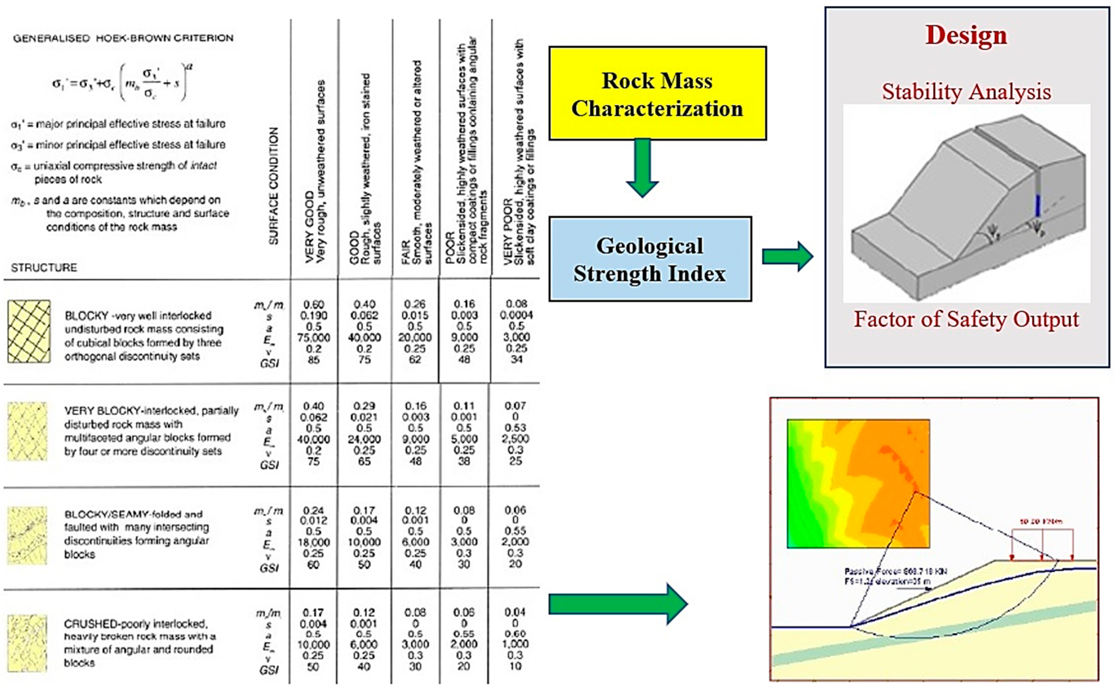
2.1. Geological Strength Index (GSI)

Unless a rock mass failure criterion could be connected to a geological description that engineering geologists could make quickly, it would be of no practical use. The geological strength index (GSI) is a system for classifying rocks that was created in the field of rock engineering to address the requirement for accurate estimation of the attributes of rocks for the design of engineering projects [15]. The foundation of the GSI system is an in-depth engineering geology description of the rock mass encountered in engineering projects. Structure and the condition of discontinuities in the rock mass, which can be determined through visual inspection of the rock mass exposed in outcrops, are two essential criteria that determine the value of the GSI [21]. The basic GSI chart’s use entails some subjectivity because there are not any quantifiable or more representative metrics, linked interval limits, or ratings for describing the rock structure and surface conditions of the discontinuities. In order to make the method easier to use, particularly for new engineers, numerous publications [18,22,23] presented quantitative GSI charts to quantify the estimation of GSI. In circumstances when there are only one or two sets of discontinuities, the GSI should not be utilized. Instead, it should only be employed when the rock mass is intact or heavily joined. When working with blocky rock masses that have minimum anisotropy, extreme caution should be used. However, it is occasionally reasonable to assign the GSI to the entire rock mass and include the single discontinuity as a layer element in the numerical model for a rock mass that has a single well-defined discontinuity [20]. According to the definition of GSI and subsequent application, it is independent of the water inflow and the in situ stress state. As mentioned, GSI has limits, as do any categorization systems, including the differences in the results of individuals. Others have suggested that the generic GSI may not appropriately reflect the size of the rock mass problem because its parameters, particularly RQD and J_Cond, are scale-dependent [24,25].

The two main geological elements behind GSI were the surface conditions of discontinuities and their shear strength, as well as the rock mass structure, which represented the degree of fracture [26]. GSI subsequently replaced RMR in the Hoek–Brown failure criterion. To encourage early adoption, Hoek et al. [15,27] provided the following relationships for estimating GSI, termed GSI_calc in this paper from RMR and Q’:

GSI_calc = RMR₈₉ − 5

(1)

for RMR₈₉ ≥ 23

GSI_calc = 9lnQ’ + 44

(2)

for RMR₈₉ < 23

GSI was developed to assess tunnel and slope faces using charts (Figure 3) and cannot be estimated directly from the characterization of the drill core. Equations (1) and (2) also enable the estimation of GSI_calc from the drill core.

Hoek et al. [19] suggested quantifying the GSI chart as a function of RQD and the joint condition parameters presented by either [1]: JCond₈₉ from RMR₈₉ or Barton et al. [14]; J_r and J_a from Q and Q-slope, on the premise that professionals with less expertise and who are “less at ease with the qualitative descriptions” may utilize this new GSI chart. The suggested equations included [18]:

GSI₂₀₁₃ = 1.5JCond₈₉ + RQD/2

(3)

$$\mathrm{GSI}2013=\frac{52{\mathrm{J}}_{\mathrm{r}}/{\mathrm{J}}_{\mathrm{a}}}{\left(1+\frac{{\mathrm{J}}_{\mathrm{r}}}{{\mathrm{J}}_{\mathrm{a}}}\right)}+ \mathrm{RQD}/2$$

(4)

Vásárhelyi et al. [28] and Somodi et al. [29] discovered that visual observation by an expert engineering geologist is the best technique to estimate GSI, compared to the computational and estimation methods examined. Moreover, Deák et al. [30] and Somodi et al. [31] analyzed the relationship between the parameters of the Q-system and the GSI value and the equations are suggested based on the empirical results of different rock engineering projects in Hungary and Australia.

Bertuzzi et al. [32] observed a decent connection between the GSI values derived by the chart (GSI_chart) and the GSI quantified (GSI₂₀₁₃) using the Hoek et al. [18] technique (Figure 3). Santa et al. [33] compared the differences between the latest edition of GSI₂₀₁₃ and the prior version (GSI₉₈) in an anisotropic media. They discovered that the 2013 version [18] allocated lower GSI ratings to rock masses with lesser quality and higher values to rock masses with greater quality. Winn et al. [34] revealed that the three alternative techniques proposed by [22,23] for a sedimentary rock mass in a Singapore dive, a variety of outcomes comparable to the field-assessed qualitative GSI, showing their good performance. However, Winn et al. [34] established a new GSI relationship by replacing RQD/2 with RQD/3 in the calculation of GSI₂₀₁₃, which provided substantially higher GSI values that did not correspond to the qualitative field values.

Figure 3. (a) GSI chart for jointed rocks [35]. (b) Quantification of GSI through joint conditions and RQD [18].

Figure 3. (a) GSI chart for jointed rocks [35]. (b) Quantification of GSI through joint conditions and RQD [18].

Yang and Elmo [36] argue against the quantification paradigm for GSI determination without taking into account the constraints of the idea that GSI quantification approaches may convert subjectivity into objectivity since the parameters under consideration are not quantitative measurements.

2.2. The Q-Slope Method

Barton and Bar [37] are credited with developing the Q-slope, an empirical engineering method for assessing the stability of rock slopes that allows for immediate access to stability with few presumptions. It is descended from the Q-system, which has been used globally for over 40 years to characterize rock exposures, drill core, and tunnels that are under construction [14,38]. Q-slope allows engineering geologists and rock engineers to analyze the stability of excavated rock slopes in the field and make prospective slope angle adjustments as rock mass conditions become obvious during construction [37,39]. The Q_slope used Q system components to slope stability assessments are calculated using the expression [16]:

$${\mathrm{Q}}_{\mathrm{slope}} =\frac{\mathrm{RQD}}{{\mathrm{J}}_{\mathrm{n}}}\times {\left(\frac{{\mathrm{J}}_{\mathrm{r}}}{{\mathrm{J}}_{\mathrm{a}}}\right)}_{\mathrm{O}}\times \frac{{\mathrm{J}}_{\mathrm{wice}}}{{\mathrm{SRF}}_{\mathrm{slope}}}$$

(5)

RQD, J_n, J_r, and J_a are the same four parameters used in Q-system. On the other hand, the frictional resistance pair Jr and Ja as necessary, each side of a wedge that may be unstable will receive this treatment. If suitable, simple orientation variables such as (J_r/J_a)_O give an estimate of the reduction in overall whole-wedge frictional resistance. The term J_w, which has now been modified to J_wice, refers to a broader range of environmental conditions ideal for rock slopes exposed to the elements for a long time. Extremes of erosive rains and ice wedging, which can occur periodically at opposing extremities of the rock-type and regional spectrum, are examples of these situations. Slope-relevant SRF classifications are also available in slope surface conditions, stress–strength ratios and major discontinuities such as faults, weakness zones or joint swarms [37].

Q’ and Q-slope’ are estimated using Equations (6) and (7), which merely remove the water, environment, stress, and strength reduction factors from the full Q-system and Q-slope equations:

$$\mathrm{Q}’=\left(\frac{\mathrm{RQD}}{{\mathrm{J}}_{\mathrm{n}}}\right)\times \left(\frac{{\mathrm{J}}_{\mathrm{r}}}{{\mathrm{J}}_{\mathrm{a}}}\right)$$

(6)

$$\mathrm{Q-slope}’=\left(\frac{\mathrm{RQD}}{{\mathrm{J}}_{\mathrm{n}}}\right)\times {\left(\frac{{\mathrm{J}}_{\mathrm{r}}}{{\mathrm{J}}_{\mathrm{a}}}\right)}_{\mathrm{A}}\times {\left(\frac{{\mathrm{J}}_{\mathrm{r}}}{{\mathrm{J}}_{\mathrm{a}}}\right)}_{\mathrm{B} \mathrm{where} \mathrm{applicable}}$$

(7)

where RQD = rock quality designation (%).

• J_n = joint set number.
• J_r = joint roughness number.
• J_a = joint alteration number.

Q-system and Q-slope ratings for RQD, J_n, J_r, and J_a are described by Barton et al. [14] and Bar and Barton [16]. These parameters are commensurate with the primary factors in GSI: rock mass structure and discontinuity surface conditions.

The main distinction between Q and Q-slope is that Q uses J_r/J_a from the collection of discontinuities with the least favorable discontinuities. In contrast, J_r/J_a for both sides (A and B) of the wedge can be considered necessary when wedges are encountered while utilizing Q-slope. In order to predict various parameters from others in material sciences and engineering properties of various rock types from their petrographic characteristics in engineering geology and rock mechanics, several researchers have attempted to construct various soft computing models [40,41,42,43]. Recent research has examined the relationships between the Q-system, Q-slope, and GSI as well as for other rocks by employing statistical analyses and various soft computing techniques such as root mean squared error value (RMSE), the mean absolute percentage error (MAPE), mean absolute error (MAE), and coefficient of determination (R-squared).

3. Study Area

The current study reviews over 192 case records collected from across 11 countries on five continents to investigate the relationship between the GSI obtained using the popular chart methods in more depth. (GSI_chart) and its correlation with Q’ and Q-slope’.

The case records were obtained from rock slope faces that were assessed during the Q-slope method development [16] from a range of mining commodities, including gold, copper, iron ore, coal, and diamonds, and civil engineering applications, including roads, highways, and quarries. GSI was estimated for these case studies using GSI chart for jointed rocks (GSI_chart). Figure 4 graphically illustrates the results from a selection of case studies. The case records include over 20 different rock types in vastly different engineering geological, environmental, and climatic settings:

• Igneous rocks include andesite, basalt, diorite, granite, kimberlite, monzodiorite, rhyolite, and tuff.
• Sedimentary rocks include chert, greywacke, limestone, mudstone, siltstone, sandstone, and banded iron formation.
• Metamorphic rocks include marble, metasandstone, phyllite, quartzite, schist, and shale.

Figure 5 presents a selection of photographs of rock slopes hosted within vastly different rock masses and their respective GSI, Q-slope, and Q-slope’ ratings for context:

• Case records A and B are both granites. A is massive whilst B is blocky.
• Case records C, D, and E are all siltstones, which are blocky, seamy, and very blocky, respectively. Joint surface quality reduces from very good to good in C and E to fair in F.
• Case record F is a sheared mudstone comprising claystones and siltstones with slickensided, graphitic infilling along bedding planes and bedding shears.
• Case records B and C have the same GSI, but vastly different Q-slope values, due to the orientation of the discontinuities.
• Case records D and E have different GSI and Q-slope’ values, but very similar Q-slope values. Both are stable slopes with bench face angles of approximately 65°.

Data analysis was conducted using SPSS23 software to outline the relations between parameters and describe the frequency distribution of GSI values [44]. Three rock types were picked and tested independently, and reliability analyses were also made. Figure 6 indicates the frequency distribution of GSI values, and

Table 1. Statistical analysis of measured GSI values.

	Number of Estimates	Median	Minimum	Maximum
Igneous	26	65	27	89
Sedimentary	139	55	20	85
Metamorphic	27	60	30	90
Total	192	55	20	90

indicates the statistical analysis of the data for all the rocks and each type of rocks separately. According to Table 1, GSI values range between 20 and 90 for all the rock types, indicating that our datasets include very good through very poor rock mass.

4. Derived Relationships between the Different Methods

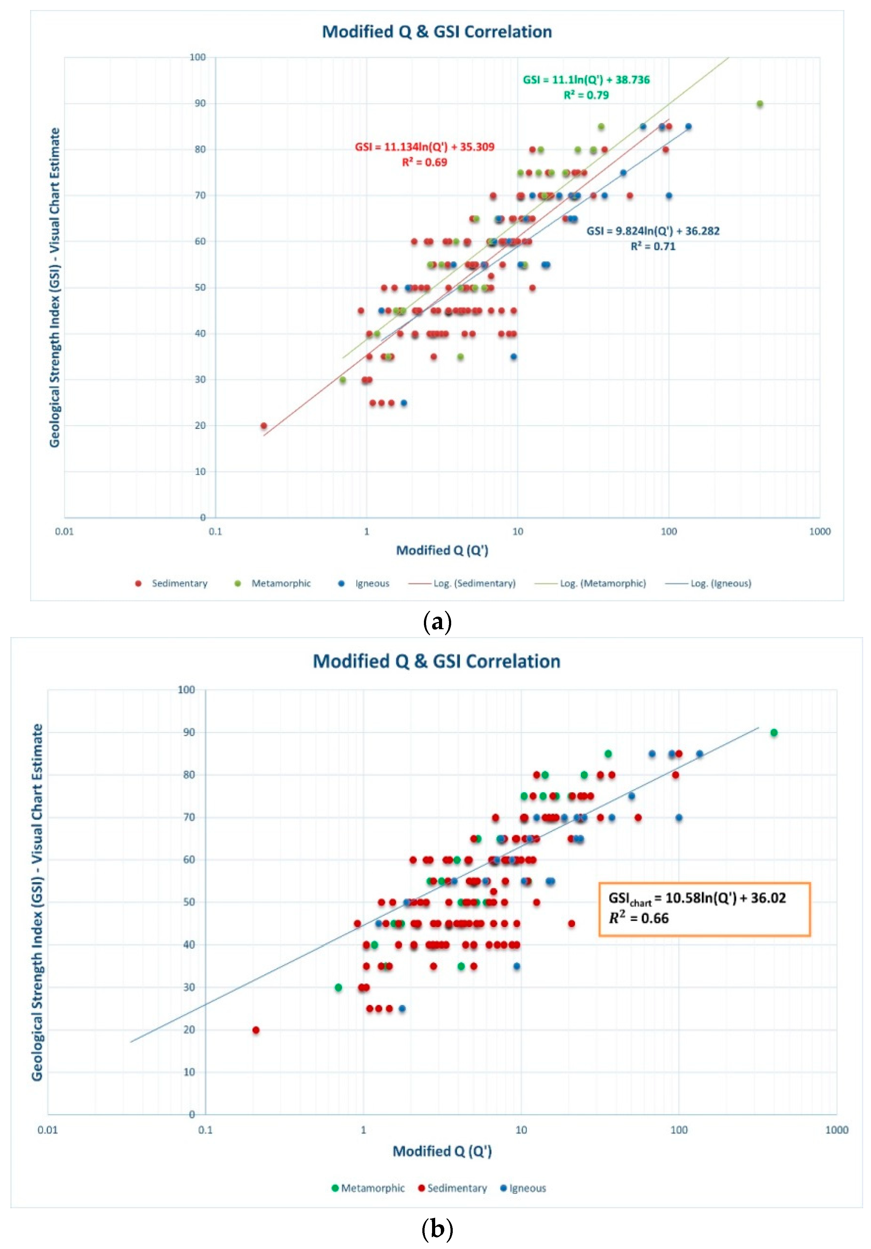
4.1. Correlation between GSI and Q’

The Q’ values were calculated by using Equation (6) and correlated to the GSI_chart. These results are summarized in Figure 7. Figure 7a shows the correlation for three types of rocks (igneous, sedimentary, and metamorphic) separately, and Figure 7b shows the correlation for all rocks together. The more reliable correlation relates to metamorphic rocks (R² = 79%). Also, for all cases, the best fitting is in logarithmic. These relationships have similarities with Equation (2).

4.2. Correlation between GSI and Q-Slope’

In addition, using Equation (7), the Q-slope’ values were calculated and correlated to the GSI_chart. Figure 8 summarizes these findings. Figure 8a shows the correlation for three different types of rocks (igneous, sedimentary, metamorphic), while Figure 8b shows the correlation for all rocks combined. The more reliable correlation is with metamorphic rocks (R² = 63%). Also, in all cases, the best fitting is logarithmic. These relationships also have similarities with Equation (2).

4.3. Correlation between GSI_chart and GSI₂₀₁₃

Furthermore, Equation (3) was used to produce the GSI₂₀₁₃ values, which were then compared with GSI_chart. Figure 9 summarizes the findings. Figure 9a depicts the correlation for three different types of rocks (igneous, sedimentary, metamorphic), while Figure 9b depicts the correlation for all rocks. Metamorphic rocks have a more reliable correlation (R² = 88%). In addition, the optimal fitting is linear in all circumstances.

5. Key Findings

Several different relationships between GSI (GSI_chart) and Q’ and Q-slope’ have been identified using over 200 new case records. The relationship between the GSI value and the Q value is:

GSI = A ln(Q) + B,

(8)

where A and B are material constants, depending on the rock type [30].

• For Q’: A and B values range from 9.82 to 11.13 and from 35.31 to 38.74, respectively.
• For Q-slope’: A and B values range from 6.23 to 8.39 and from 42.19 to 47.34, respectively.

All derived relationships are summarized in

Table 2. Empirical equations derived in this study.

Types of Correlation	Equation	R2
GSIchart & Q’ for Metamorphic rocks	GSI = 11.10ln(Q’) + 38.74	0.79
GSIchart & Q’ for Sedimentary rocks	GSI = 11.13ln(Q’) + 35.31	0.69
GSIchart & Q’ for Igneous rocks	GSI = 9.82ln(Q’) + 36.28	0.71
GSIchart & Q’ for all rocks	GSI = 10.58ln(Q’) + 36.02	0.66
GSIchart & Q-slope’ for Metamorphic rocks	GSI = 7.98ln(Q-slope’) + 47.34	0.63
GSIchart & Q-slope’ for Sedimentary rocks	GSI = 8.39ln(Q-slope’) + 42.19	0.60
GSIchart & Q-slope’ for Igneous rocks	GSI = 6.23ln(Q-slope’) + 44.94	0.58
GSIchart & Q-slope’ for all rocks	GSI = 8.13ln(Q-slope’) + 44.12	0.62
GSIchart & GSI2013 for Metamorphic rocks	GSI2013 = 0.98(GSIchart) − 0.51	0.88
GSIchart & GSI2013 for Sedimentary rocks	GSI2013 = 1.03(GSIchart) + 1.19	0.74
GSIchart & GSI2013 for Igneous rocks	GSI2013 = 0.95(GSIchart) + 8.41	0.71
GSIchart & GSI2013 for all rocks	GSI2013 = 0.97(GSIchart) + 4.29	0.75

.

6. Quantitative Relationships and Errors

Four common statistical metrics, including determination coefficient (R²), root mean square error (RMSE), mean absolute error (MAE), and mean absolute percent error (MAPE), were used to assess the statistical efficiency of the GSI_chart prediction in the training and testing sets [45]. Equations (9)–(11) specify the following performance measures:

$$\mathrm{RMSE} =\sqrt{\frac{{{\displaystyle \sum }}_{\mathrm{i}=1}^{\mathrm{n}}{\left(\mathrm{pi}-\mathrm{qi}\right)}^2}{\mathrm{n}}}$$

(9)

$$\mathrm{MAPE} =\frac{1}{\mathrm{n}}{{\displaystyle \sum }}_{\mathrm{i}=1}^{\mathrm{n}}\left|\frac{\mathrm{qi}-\mathrm{pi}}{\mathrm{qi}}\right|\times 100$$

(10)

$$\mathrm{MAE} =\frac{{{\displaystyle \sum }}_{\mathrm{i}=1}^{\mathrm{n}}\left|\mathrm{pi}-\mathrm{qi}\right|}{\mathrm{n}}$$

(11)

Here, p_i and q_i stand in for the i_th predicted and expected results, respectively, and n denotes the total number of experiments. Since significant errors are dealt with far more successfully than smaller ones, RMSE is a widely used metric. When the RMSE approaches 0, it means that the prediction error was minimal. However, it does not always guarantee top performance. Additionally, MAE was calculated and is incredibly helpful when data are smooth and continuous [46].

Plotting the residuals vs. the fitted values of the dependent variable allows one to assess the error of the proposed model. The residuals are the discrepancies between the experimental outcomes and the values that the suggested model predicted. The values that have been fitted are those that the proposed model anticipated. Figure 10 illustrates the residuals’ balanced and symmetrical dispersion about the horizontal axis.

Additionally, the residuals’ outermost points resemble a circular in shape. The residuals’ independent nature and random distribution around the centerline are confirmed by this distribution [47,48]. To make sure of this, the determination coefficient, R-squared, is computed. It turns out to be very nearly equivalent to zero. In other words, the residuals are not dependent on one another. The proposed model’s goodness of fit is therefore excellent.

The calculations: These new statistical indicators that provide quantitative connections between GSI_chart and Q’ and Q-slope’, as well as GSI₂₀₁₃, are given in

Table 3. Statistical indicators for Q-slope’ vs. GSI_chart, Q’ vs. GSI_chart, and GSI_calc vs. GSI_chart models.

Statistical Metrics	Q-Slope’ vs. GSIchart		Q’ vs. GSIchart		GSIcalc vs. GSIchart
	Training	Testing	Training	Testing	Training	Testing
RMSE	9.93	10.8	8.5	9.56	7.47	7.85
MAPE	0.16	0.18	0.13	0.16	0.11	0.11
MAE	7.87	8.5	6.69	7.8	5.95	5.9

.

7. Conclusions

The relationships between the geological strength index (GSI) and the Q-system and Q-slope are explored in this paper. Quantitative correlation analyses have been carried out systematically using study data from various igneous, metamorphic, and sedimentary rocks.

Validated results show that the proposed simplified quantitative correlations accurately reflect the observed relationship between the mentioned parameters.

The statistical measures employed to assess the effectiveness of the model were mean absolute error (MAE), mean absolute percentage error (MAPE), and root means square error (RMSE). These indicators have various relationships: the logarithmic equations provide good forecasting results between GSI_chart and Q’ and Q-slope’, while the linear equations between GSI_chart and GSI₂₀₁₃ fall in the “stronger prediction” category.

These correlations can be used to assess the surrounding rock mass of various rock types in various places. While these and other connections are likely relevant elsewhere in similar ground conditions, readers are strongly recommended to validate them at their local site before using them. Thus, it is strongly encouraged that engineering geologists and geotechnical engineers have to develop a site-specific correlations chart at various locations.

References

1. Bieniawski, Z.T. Engineering Rock Mass Classifications: A Complete Manual for Engineers and Geologists in Mining, Civil, and Petroleum Engineering; Wiley: New York, NY, USA, 1989. [Google Scholar]
2. Duncan, J.M. State of the Art: Limit Equilibrium and Finite-Element Analysis of Slopes. J. Geotech. Eng. 1996, 122, 577–596. [Google Scholar] [CrossRef]
3. Lauffer, H. Gebirgsklassifizierung für den Stollenbau. Geol. Bauwes. 1958, 24, 46–51. [Google Scholar]
4. Eberhardt, E. Geological Engineering Practice I—Rock Engineering, Lecture 5 [PowerPoint Slides]. 2017. Available online: https://www.eoas.ubc.ca/courses/eosc433/lecture-material/L5-EmpiricalDesign.pdf (accessed on 1 June 2017).
5. Hoek, E. Reliability of Hoek-Brow estimates of Rock Mass properties and their impact design. Int. J. Rock Mech. Min. Sci. Geomech. Abst. 1998, 35, 63–68. [Google Scholar] [CrossRef]
6. Ván, P.; Vásárhelyi, B. Sensitivity analysis of GSI based mechanical parameters of the rock mass. Period. Polytech. Civ. Eng. 2014, 58, 379–386. [Google Scholar] [CrossRef] [Green Version]
7. Romana, M.; Serón, J.B.; Montalar, E. SMR Geomechanics Classification: Application, Experience and Validation. In Proceedings of the 10th ISRM Congress, Sandton, South Africa, 8–12 September 2003. [Google Scholar]
8. Romana, M. New adjustment ratings for application of Bieniawski classification to slopes. In Proceedings of the International Symposium on Role of Rock Mechanics, Zacatecas, Mexico, 2–4 September 1985; pp. 49–53. [Google Scholar]
9. Tomás, R.; Delgado, J.; Serón, J. Modification of slope mass rating (SMR) by continuous functions. Int. J. Rock Mech. Min. Sci. 2007, 44, 1062–1069. [Google Scholar] [CrossRef]
10. Tomas, R.; Cuenca, A.; Cano, M.; García-Barba, J. A graphical approach for slope mass rating (SMR). Eng. Geol. 2012, 124, 67–76. [Google Scholar] [CrossRef]
11. Taheri, A.; Tani, K. A Modified rock mass classification system for preliminary design of rock slopes. In Proceedings of the 4th Asian Rock Mechanics Symposium, Singapore, 8–10 November 2006. [Google Scholar]
12. Taheri, A. A rating system for preliminary design of rock slopes. In Proceedings of the 41st Japan Geotechnical Society Conference (JGS), Kagoshima, Japan, 12–15 July 2006. [Google Scholar]
13. Santos, A.E.M.; Lana, M.S.; Pereira, T.M. Evaluation of machine learning methods for rock mass classification. Neural Comput. Appl. 2022, 34, 4633–4642. [Google Scholar] [CrossRef]
14. Barton, N.R.; Lien, R.; Lunde, J. Engineering classification of rock masses for the design of tunnel support. Rock Mech. 1974, 6, 189–239. [Google Scholar] [CrossRef]
15. Hoek, E. Strength of rock and rock masses. ISRM News J. 1994, 2, 4–16. [Google Scholar]
16. Bar, N.; Barton, N. The Q-slope Method for Rock Slope Engineering. Rock Mech. Rock Eng. 2017, 50, 3307–3322. [Google Scholar] [CrossRef]
17. Somodi, G.; Bar, N.; Kovács, L.; Arrieta, M.; Török, Á.; Vásárhelyi, B. Study of Rock Mass Rating (RMR) and Geological Strength Index (GSI) Correlations in Granite, Siltstone, Sandstone and Quartzite Rock Masses. Appl. Sci. 2021, 11, 3351. [Google Scholar] [CrossRef]
18. Hoek, E.; Carter, T.G.; Diederichs, M.S. Quantification of the geological strength index chart. In Proceedings of the 47th US Rock Mechanics/Geomechanics Symposium—ARMA 2013 (ARMA 13–672), San Francisco, CA, USA, 23–26 June 2013. [Google Scholar]
19. Hoek, E.; Brown, E.T. Empirical Strength Criterion for Rock Masses. J. Geotech. Eng. 1980, 106, 1013–1035. [Google Scholar] [CrossRef]
20. Hoek, E.; Brown, E.T. The Hoek-Brown Failure Criterion—A 1988 Update. In Proceedings of the 15th Canadian Rock Mechanics Symposium; University of Toronto: Toronto, ON, Canada, 1988; pp. 31–38. [Google Scholar]
21. Jianping, Z.; Jiayi, S. The Hoek-Brown Failure Criterion—From Theory to Application; Springer: Berlin/Heidelberg, Germany, 2018. [Google Scholar]
22. Sonmez, H.; Ulusay, R. Modifications to the Geological Strength Index (GSI) and their applicability to the stability of slopes. Int. Rock Mech. Min. Sci. 1999, 36, 743–760. [Google Scholar] [CrossRef]
23. Cai, M.; Kaiser, P.K.; Uno, H.; Tasaka, Y.; Minami, M. Estimation of Rock Mass Deformation Modulus and Strength of Jointed Hard Rock Masses using the GSI system. Int. J. Rock Mech. Min. Sci. 2004, 41, 3–19. [Google Scholar] [CrossRef]
24. Hudson, J.; Harrison, J. Engineering Rock Mechanics; Pergamon: Bergama, Turkey, 1997. [Google Scholar]
25. Mostyn, G.; Douglas, K. Strength of intact rock and rock masses. In Proceedings of the ISRM International Symposium, Melbourne, Australia, 19–24 November 2000. [Google Scholar]
26. Renani, H.R.; Cai, M. Forty-Year Review of the Hoek-Brown Failure Criterion for Jointed Rock Masses. Rock Mech. Rock Eng. 2022, 55, 439–461. [Google Scholar] [CrossRef]
27. Hoek, E.; Kaiser, P.K.; Bawden, W.F. Support of Underground Excavations in Hard Rock; Balkema: Rotterdam, The Netherlands, 1995. [Google Scholar]
28. Vásárhelyi, B.; Somodi, G.; Krupa, Á.; Kovács, L. Determining the Geological Strength Index (GSI) using different methods. In Proceedings of the ISRM International Symposium—EUROCK 2016, Nevsehir, Turkey, 29–31 August 2016; pp. 1049–1054. [Google Scholar]
29. Somodi, G.; Krupa, Á.; Kovács, L.; Vásárhelyi, B. Comparison of different calculation methods of Geological Strength Index (GSI) in a specific underground construction site. Eng. Geol. 2018, 243, 50–58. [Google Scholar] [CrossRef]
30. Deák, F.; Kovács, L.; Vásárhelyi, B. Geotechnical rock mass documentation in the Bátaapáti radioactive waste repository. Cent. Eur. Geol. 2014, 57, 197–211. [Google Scholar] [CrossRef] [Green Version]
31. Somodi, G.; Bar, N.; Vásárhelyi, B. Correlation between the rock mass quality (Q-system) method and Geological Strength Index (GSI). In Proceedings of the Fifth Symposium of the Macedonian Association for Geotechnics, ISRM Specialized Conference, Ohrid, North Macedonia, 23–25 June 2022; pp. 461–468. [Google Scholar]
32. Bertuzzi, R.; Douglas, K.; Mostyn, G. Comparison of quantified and chart GSI for four rock masses. Eng. Geol. 2016, 202, 24–35. [Google Scholar] [CrossRef]
33. Santa, C.; Gonçalves, L.; Chaminé, H.I. A comparative study of GSI chart versions in a heterogeneous rock mass media (Marão tunnel, North Portugal): A reliable index in geotechnical surveys and rock engineering design. Bull. Eng. Geol. Environ. 2019, 78, 5889–5903. [Google Scholar] [CrossRef]
34. Winn, K.; Ngai, L.; Wong, Y. Quantitative GSI determination of Singapore’s sedimentary rock mass by applying four different approaches. Geotech. Geol. Eng. 2019, 37, 2103–2119. [Google Scholar] [CrossRef]
35. Hoek, E.; Marinos, P. Predicting tunnel squeezing. Tunn. Tunn. Int. 2000, 32, 45–51. [Google Scholar]
36. Yang, B.; Elmo, D. Why Engineers Should Not Attempt to Quantify GSI. Geosciences 2022, 12, 417. [Google Scholar] [CrossRef]
37. Barton, N.; Bar, N. Introducing the Q-Slope Method and Its Intended Use within Civil and Mining Engineering Projects. In Future Development of Rock Mechanics, Proceedings of the ISRM Regional Symposium Eurock 2015 and 64th Geomechanics Colloquium, Salzburg, Austria, 7–10 October 2015; Schubert, W., Kluckner, A., Eds.; GEOAUSTRIA: Salzburg, Austria, 2015; pp. 157–162. ISBN 978-3-9503898-1-4. [Google Scholar]
38. Barton, N.R.; Grimstad, E. An Illustrated Guide to the Q-System Following 40 Years Use in Tunnelling; In-House Publishing: Oslo, Norway, 2014. [Google Scholar]
39. Bar, N.; Barton, N. Q-Slope: An Empirical Rock Slope Engineering Approach in Australia. Austr. Geomech. 2018, 53, 73–86. [Google Scholar]
40. Moustafa, E.B.; Hammad, A.H.; Elsheikh, A.H. A new optimized artificial neural network model to predict thermal efficiency and water yield of tubular solar still. Case Stud. Therm. Eng. 2022, 30, 101750. [Google Scholar] [CrossRef]
41. Abdolrasol, M.G.; Hussain, S.S.; Ustun, T.S.; Sarker, M.R.; Hannan, M.A.; Mohamed, R.; Ali, J.A.; Mekhilef, S.; Milad, A. Artificial neural networks based optimization techniques: A review. Electronics 2021, 10, 2689. [Google Scholar] [CrossRef]
42. Cantisani, E.; Garzonio, C.A.; Ricci, M.; Vettori, S. Relationships between the petrographical, physical and mechanical properties of some Italian sandstones. Int. J. Rock Mech. Min. Sci. 2013, 60, 321–332. [Google Scholar] [CrossRef]
43. Cowie, S.; Walton, G. The effect of mineralogical parameters on the mechanical properties of granitic rocks. Eng. Geol. 2018, 240, 204–225. [Google Scholar] [CrossRef]
44. IBM Corp. Released 2015. IBM SPSS Statistics for Windows, Version 23.0; IBM Corp: Armonk, NY, USA, 2015. [Google Scholar]
45. Agbulut, Ü.; Gürel, A.E.; Biçen, Y. Prediction of daily global solar radiation using different machine learning algorithms: Evaluation and comparison. Renew. Sustain. Energy Rev. 2021, 135, 110114. [Google Scholar] [CrossRef]
46. Shahin, M.A. Use of evolutionary computing for modelling some complex problems in geotechnical engineering. Geomech. Geoengin. 2015, 10, 109–125. [Google Scholar] [CrossRef] [Green Version]
47. Khalaf, A.A.; Kopecskó, K. Modelling of Modulus of Elasticity of Low-Calcium-Based Geopolymer Concrete Using Regression Analysis. Adv. Mater. Sci. Eng. 2022, 2022, 4528264. [Google Scholar] [CrossRef]
48. Motulsky, H.J.; Ransnas, L.A. Fitting curves to data using nonlinear regression: A practical and nonmathematical review. FASEB J. 1987, 1, 365–374. [Google Scholar] [CrossRef] [PubMed]
Figure 1. Rock mass characterization vs. Classification for rock slopes [4].
Sustainability 15 11233 g001
Figure 2. Estimation of constants mb/mi, s, a, deformation modulus E, and the Poisson’s ratio (ν) for the generalized Hoek–Brown failure criterion based upon rock mass structure and discontinuity surface conditions used for the design stage [4].
Sustainability 15 11233 g002
Figure 4. Case records: geographic location and industry and commodity. (The numbers indicate the locations of sampling).
Sustainability 15 11233 g004
Figure 5. Selection of case studies comparing GSI, Q-slope, and Q-slope’.
Sustainability 15 11233 g005
Figure 6. Histogram of measured GSI for (a) igneous rocks, (b) sedimentary rocks, (c) metamorphic rocks, and (d) all the rock types.
Sustainability 15 11233 g006
Figure 7. Relationships between GSIchart and Q’: (a) separated for igneous, sedimentary, metamorphic rocks, (b) for all rocks.
Sustainability 15 11233 g007
Figure 8. Relationships between GSIchart and Q-slope’: (a) separated for igneous, sedimentary, metamorphic rocks, (b) for all rocks.
Sustainability 15 11233 g008
Figure 9. Relationships between GSIchart and GSI2013: (a) separated for igneous, sedimentary, metamorphic rocks, (b) for all rocks.
Sustainability 15 11233 g009
Figure 10. Distribution of the residuals against fitted values: (a) between GSIchart and Q-slope’, (b) GSIchart and Q’, (c) GSIchart and GSIcalc.
Sustainability 15 11233 g010