


How Does the COVID-19 Pandemic Impact Internal Trade? Evidence from China’s Provincial-Level Data

Abstract
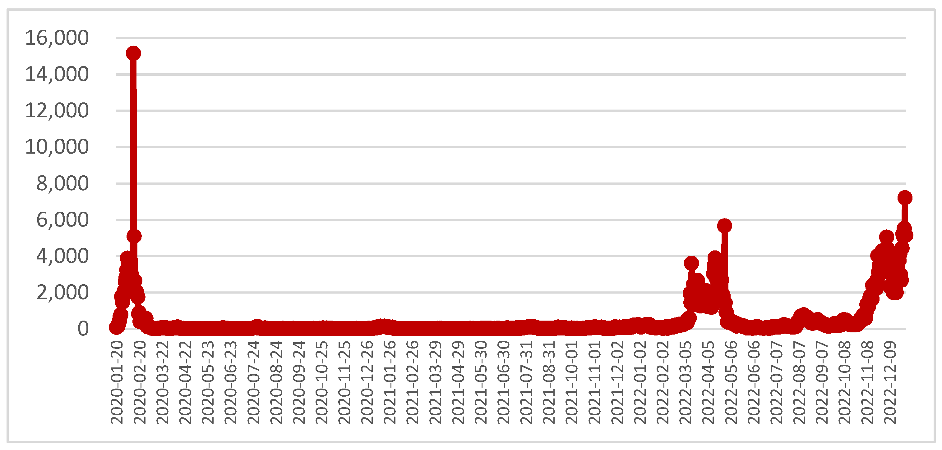
:1. Introduction
2. Basic Facts
3. Interprovincial Trade Flows and Barriers
3.1. Estimation of Interprovincial Trade Flows
3.1.1. Estimation Method
- Calculate the interregional friction coefficient for the base year.
- 2.
- Estimated total output for the target year.
- 3.
- Estimated interprovincial trade flows.
3.1.2. Estimation Results
3.2. Inferred Interprovincial Trade Barriers
4. The Effects of COVID-19 on Trade: Causal Inferences
4.1. COVID-19 and Interprovincial Trade Flows
4.1.1. Empirical Frameworks
4.1.2. Baseline Results
4.1.3. Robustness
4.2. COVID-19 and Interprovincial Trade Barriers
4.2.1. Empirical Frameworks
4.2.2. Estimated Results
5. Trade Barrier Effects of COVID-19: Economic Consequences
5.1. Model and Calibration
5.1.1. Model Setup
5.1.2. Calibration
5.2. Economic Effects of Changes in Trade Barriers
6. Conclusions
Author Contributions
Funding
Institutional Review Board Statement
Informed Consent Statement
Data Availability Statement
Conflicts of Interest
References
- Barbero, J.; de Lucio, J.J.; Rodríguez-Crespo, E. Effects of COVID-19 on trade flows: Measuring their impact through government policy responses. PLoS ONE 2021, 16, e258356. [Google Scholar] [CrossRef] [PubMed]
- Pei, J.; de Vries, G.; Zhang, M. International trade and COVID-19: City-level evidence from China’s lockdown policy. J. Reg. Sci. 2022, 62, 670–695. [Google Scholar] [CrossRef] [PubMed]
- Head, K.; Ries, J. Increasing returns versus national product differentiation as an explanation for the pattern of US-Canada trade. Am. Econ. Rev. 2001, 91, 858–876. [Google Scholar] [CrossRef] [Green Version]
- Baldwin, R.; Di, M.; Weder, B. Economics in the Time of COVID-19. Available online: https://cepr.org/publications/books-and-reports/economics-time-covid-19 (accessed on 1 January 2023).
- Baqaee, D.; Farhi, E. Supply and Demand in Disaggregated Keynesian Economies with an Application to the COVID-19 Crisis. Am. Econ. Rev. 2022, 112, 1397–1436. [Google Scholar] [CrossRef]
- Cakmakli, C.; Demiralp, S.; Kalemli-Ozcan, S.; Yesiltas, S.; Yildirim, M.A. COVID-19 and Emerging Markets: An Epidemiological Model with International Production Networks and Capital Flows. Available online: https://www.imf.org/en/Publications/WP/Issues/2020/07/17/COVID-19-and-Emerging-Markets-An-Epidemiological-Model-with-International-Production-49566 (accessed on 1 January 2023).
- Kejžar, K.Z.; Velić, A.; Damijan, J.P. COVID-19, trade collapse and GVC linkages: European experience. World Econ. 2022. [Google Scholar] [CrossRef] [PubMed]
- Cai, D.; Hayakawa, K. Heterogeneous Impacts of COVID-19 on trade: Evidence from China’s province-level data. J. Int. Trade Econ. Dev. 2022, 31, 1072–1085. [Google Scholar] [CrossRef]
- Fang, H.; Wang, L.; Yang, Y. Human mobility restrictions and the spread of the Novel Coronavirus (2019-nCoV) in China. J. Public Econ. 2020, 191, 104272. [Google Scholar] [CrossRef] [PubMed]
- Liu, X.; Ornelas, E.; Shi, H. The trade impact of the COVID-19 pandemic. World Econ. 2022, 45, 3751–3779. [Google Scholar] [CrossRef] [PubMed]
- Luo, S.; Tsang, K.P. China and World Output Impact of the Hubei Lockdown during the Coronavirus Outbreak. Contemp. Econ. Policy 2020, 38, 583–592. [Google Scholar] [CrossRef] [PubMed]
- Chen, J.; Chen, W.; Liu, E.K.; Luo, J.; Song, Z. The Economic Cost of Lockdown in China: Evidence from City-to-City Truck Flows. Available online: https://research-center.econ.cuhk.edu.hk/en-gb/research/research-papers/515-the-economic-cost-of-lockdown-in-china-evidence-from-city-to-city-truck-flows (accessed on 1 January 2023).
- Leontief, W.; Strout, A. Multiregional Input–Output Analysis. In Structural Interdependence and Economic Development, Proceedings of the International Conference on Input–Output Techniques, Geneva, Switzerland, 11–13 September 1961; Barna, T., Ed.; Palgrave Macmillan: London, UK, 1963; pp. 119–150. [Google Scholar]
- Li, Z.R.; Yang, R.D.; Huang, G.T. Research on Inter-provincial Trade Estimation and Trade Barriers of China. Econ. Stud. 2022, 57, 118–135. [Google Scholar]
- Zheng, H.R.; Zhang, Z.K.; Wei, W.D.; Song, M.L.; Dietzenbacher, E.; Wang, X.Y.; Meng, J.; Shan, Y.L.; Ou, J.M.; Guan, D.B. Regional determinants of China’s consumption-based emissions in the economic transition. Environ. Res. Lett. 2020, 15, 074001. [Google Scholar] [CrossRef]
- Anderson, J.E.; van Wincoop, E. Gravity with gravitas: A solution to the border puzzle. Am. Econ. Rev. 2003, 93, 170–192. [Google Scholar] [CrossRef] [Green Version]
- Allen, T.; Arkolakis, C.; Takahashi, Y. Universal Gravity. J. Political Econ. 2020, 128, 393–433. [Google Scholar] [CrossRef]
- Evenett, S.J.; Keller, W. On Theories Explaining the Success of the Gravity Equation. J. Political Econ. 2002, 110, 281–316. [Google Scholar] [CrossRef] [Green Version]
- Head, K.; Mayer, T. Chapter 3—Gravity Equations: Workhorse, Toolkit, and Cookbook. In Handbook of International Economics; Gopinath, G., Helpman, E., Rogoff, K., Eds.; Elsevier: Amsterdam, The Netherlands, 2014; Volume 4, pp. 131–195. [Google Scholar]
- Silva, J.M.C.S.; Tenreyro, S. The Log of Gravity. Rev. Econ. Stat. 2006, 88, 641–658. [Google Scholar] [CrossRef] [Green Version]
- Zhang, X.; Luo, W.; Zhu, J. Top-Down and Bottom-Up Lockdown: Evidence from COVID-19 Prevention and Control in China. J. Chin. Political Sci. 2021, 26, 189–211. [Google Scholar] [CrossRef] [PubMed]
- Poncet, S. A Fragmented China: Measure and Determinants of Chinese Domestic Market Disintegration. Rev. Int. Econ. 2005, 13, 409–430. [Google Scholar] [CrossRef] [Green Version]
- Tombe, T.; Zhu, X.D. Trade, Migration, and Productivity: A Quantitative Analysis of China. Am. Econ. Rev. 2019, 109, 1843–1872. [Google Scholar] [CrossRef] [Green Version]
- Caliendo, L.; Parro, F.; Rossi-Hansberg, E.; Sarte, P. The Impact of Regional and Sectoral Productivity Changes on the U.S. Economy. Rev. Econ. Stud. 2018, 85, 2042–2096. [Google Scholar] [CrossRef]
- Eaton, J.; Kortum, S. Technology, geography, and trade. Econometrica 2002, 70, 1741–1779. [Google Scholar] [CrossRef]
- Che, Z.; Che, J.; Wang, S. Trade Elasticity, Trade Costs and Gains from Trade: A Quantitative Analysis of China. Available online: https://ssrn.com/abstract=4167075 (accessed on 15 August 2022).


| Total Trade Flows (Trillions of RMB) | The Proportion of Trade Flows (%) | |||||||
|---|---|---|---|---|---|---|---|---|
| DO | IO | EX | IM | IO/TO | EX/TO | II/TI | IM/TI | |
| 2018 | 161.21 | 35.11 | 16.46 | 14.13 | 19.76 | 9.26 | 20.02 | 8.06 |
| 2019 | 170.48 | 36.92 | 17.24 | 14.34 | 19.67 | 9.19 | 19.98 | 7.76 |
| 2020 | 173.77 | 37.49 | 17.86 | 14.25 | 19.56 | 9.32 | 19.94 | 7.58 |
| 2021 | 187.82 | 40.29 | 21.70 | 17.34 | 19.23 | 10.36 | 19.64 | 8.45 |
| 2022 | 193.36 | 40.96 | ||||||
| Province | DO (Trillions of RMB) | IO (Trillions of RMB) | ||||||||
|---|---|---|---|---|---|---|---|---|---|---|
| 2018 | 2019 | 2020 | 2021 | 2022 | 2018 | 2019 | 2020 | 2021 | 2022 | |
| BJ | 4.71 | 5.10 | 5.14 | 5.82 | 5.82 | 1.87 | 1.99 | 2.01 | 2.22 | 2.23 |
| TJ | 3.71 | 3.88 | 3.94 | 4.19 | 4.18 | 1.01 | 1.06 | 1.08 | 1.15 | 1.16 |
| HEB | 6.60 | 6.82 | 7.03 | 7.14 | 7.31 | 1.65 | 1.71 | 1.75 | 1.82 | 1.85 |
| SX | 2.39 | 2.44 | 2.51 | 2.60 | 2.69 | 0.74 | 0.75 | 0.76 | 0.76 | 0.76 |
| IM | 4.69 | 4.35 | 3.72 | 4.39 | 4.13 | 1.60 | 1.55 | 1.42 | 1.66 | 1.60 |
| LN | 6.99 | 6.38 | 5.39 | 5.19 | 4.61 | 1.49 | 1.46 | 1.34 | 1.36 | 1.28 |
| JL | 3.03 | 3.09 | 3.24 | 3.41 | 3.21 | 1.25 | 1.29 | 1.33 | 1.42 | 1.35 |
| HLJ | 2.10 | 2.10 | 2.08 | 2.14 | 2.18 | 0.93 | 0.94 | 0.94 | 1.00 | 1.01 |
| SH | 5.36 | 5.54 | 5.59 | 5.88 | 5.79 | 2.37 | 2.45 | 2.48 | 2.62 | 2.61 |
| JS | 16.38 | 16.94 | 17.51 | 18.53 | 18.83 | 3.05 | 3.19 | 3.26 | 3.48 | 3.54 |
| ZJ | 8.05 | 8.35 | 8.58 | 8.98 | 9.13 | 1.95 | 2.05 | 2.10 | 2.23 | 2.27 |
| AH | 7.59 | 8.79 | 9.60 | 11.14 | 12.08 | 1.25 | 1.39 | 1.48 | 1.66 | 1.76 |
| FJ | 6.22 | 6.93 | 7.30 | 8.17 | 8.86 | 0.67 | 0.72 | 0.75 | 0.82 | 0.86 |
| JX | 5.48 | 5.97 | 6.28 | 6.78 | 7.16 | 1.08 | 1.16 | 1.20 | 1.30 | 1.35 |
| SD | 19.10 | 19.96 | 20.99 | 22.76 | 23.95 | 1.51 | 1.58 | 1.65 | 1.77 | 1.83 |
| HEN | 11.08 | 12.32 | 12.41 | 13.21 | 13.87 | 2.81 | 3.07 | 3.11 | 3.32 | 3.44 |
| HUB | 6.02 | 6.70 | 5.75 | 7.09 | 7.65 | 0.44 | 0.48 | 0.45 | 0.52 | 0.55 |
| HUN | 4.98 | 5.39 | 5.67 | 6.01 | 6.35 | 0.80 | 0.86 | 0.89 | 0.95 | 0.99 |
| GD | 13.52 | 14.42 | 14.80 | 16.12 | 16.36 | 2.93 | 3.10 | 3.17 | 3.44 | 3.51 |
| GX | 2.82 | 3.01 | 3.16 | 3.42 | 3.53 | 0.62 | 0.66 | 0.68 | 0.74 | 0.76 |
| HAIN | 0.54 | 0.55 | 0.57 | 0.61 | 0.60 | 0.22 | 0.23 | 0.23 | 0.25 | 0.25 |
| CQ | 3.07 | 3.35 | 3.58 | 3.99 | 4.14 | 1.00 | 1.08 | 1.13 | 1.24 | 1.28 |
| SC | 6.08 | 6.60 | 6.94 | 7.48 | 7.71 | 0.51 | 0.54 | 0.56 | 0.61 | 0.62 |
| GZ | 2.05 | 2.39 | 2.62 | 3.01 | 3.04 | 0.70 | 0.79 | 0.85 | 0.96 | 0.98 |
| YN | 1.86 | 2.02 | 2.12 | 2.23 | 2.34 | 0.31 | 0.33 | 0.34 | 0.36 | 0.37 |
| TIB | 0.11 | 0.13 | 0.15 | 0.16 | 0.16 | 0.03 | 0.03 | 0.03 | 0.03 | 0.03 |
| SXX | 3.37 | 3.57 | 3.64 | 3.82 | 4.02 | 1.32 | 1.40 | 1.42 | 1.50 | 1.56 |
| GS | 1.02 | 1.01 | 1.01 | 0.98 | 0.99 | 0.27 | 0.27 | 0.27 | 0.27 | 0.27 |
| QH | 0.35 | 0.37 | 0.37 | 0.38 | 0.39 | 0.05 | 0.06 | 0.06 | 0.06 | 0.06 |
| NX | 0.47 | 0.50 | 0.52 | 0.55 | 0.57 | 0.16 | 0.17 | 0.17 | 0.18 | 0.19 |
| XJ | 1.46 | 1.52 | 1.59 | 1.66 | 1.71 | 0.51 | 0.54 | 0.56 | 0.59 | 0.60 |
| Province | IO/TO (%) | EX/TO (%) | ||||||
|---|---|---|---|---|---|---|---|---|
| 2018 | 2019 | 2020 | 2021 | 2018 | 2019 | 2020 | 2021 | |
| BJ | 38.11 | 37.66 | 37.66 | 36.04 | 3.83 | 3.46 | 3.81 | 5.39 |
| TJ | 25.25 | 25.52 | 25.60 | 25.25 | 7.60 | 6.83 | 6.64 | 8.12 |
| HEB | 23.86 | 23.97 | 23.75 | 24.02 | 4.73 | 4.63 | 4.68 | 5.70 |
| SX | 29.82 | 29.65 | 29.28 | 27.47 | 4.38 | 3.99 | 3.76 | 5.75 |
| IM | 33.83 | 35.29 | 37.67 | 37.39 | 1.04 | 1.16 | 1.19 | 1.41 |
| LN | 20.21 | 21.51 | 23.44 | 24.38 | 5.20 | 5.69 | 5.56 | 6.92 |
| JL | 40.81 | 41.19 | 40.76 | 41.09 | 1.21 | 1.16 | 0.98 | 1.09 |
| HLJ | 43.53 | 44.20 | 44.62 | 45.45 | 1.50 | 1.82 | 1.76 | 2.26 |
| SH | 36.08 | 36.51 | 36.75 | 36.44 | 18.27 | 17.47 | 17.12 | 18.17 |
| JS | 15.92 | 16.16 | 16.10 | 15.97 | 14.42 | 14.10 | 13.54 | 14.96 |
| ZJ | 19.12 | 19.18 | 19.06 | 18.71 | 21.24 | 21.90 | 22.04 | 24.79 |
| AH | 15.96 | 15.38 | 14.91 | 14.36 | 3.08 | 3.03 | 3.32 | 3.71 |
| FJ | 9.69 | 9.43 | 9.28 | 8.96 | 10.05 | 9.77 | 9.49 | 11.06 |
| JX | 19.13 | 18.86 | 18.45 | 18.36 | 3.15 | 3.26 | 3.70 | 4.34 |
| SD | 7.44 | 7.49 | 7.41 | 7.18 | 5.67 | 5.58 | 5.57 | 7.48 |
| HEN | 24.53 | 24.14 | 24.21 | 24.15 | 3.34 | 3.21 | 3.54 | 4.04 |
| HUB | 7.09 | 6.97 | 7.48 | 7.02 | 3.36 | 3.18 | 4.38 | 4.42 |
| HUN | 15.69 | 15.44 | 15.18 | 15.21 | 2.72 | 3.26 | 3.60 | 3.92 |
| GD | 16.10 | 16.01 | 15.83 | 15.69 | 25.73 | 25.62 | 26.06 | 26.53 |
| GX | 21.08 | 21.00 | 20.70 | 20.50 | 3.98 | 4.24 | 4.43 | 5.40 |
| HAIN | 38.43 | 38.73 | 38.88 | 38.66 | 5.41 | 5.72 | 4.65 | 4.49 |
| CQ | 29.66 | 29.20 | 28.49 | 27.81 | 9.03 | 9.30 | 9.59 | 10.46 |
| SC | 7.91 | 7.81 | 7.63 | 7.55 | 4.94 | 5.23 | 6.14 | 6.67 |
| GZ | 33.49 | 32.59 | 31.87 | 31.40 | 1.82 | 1.48 | 1.53 | 1.54 |
| YN | 16.06 | 15.56 | 15.30 | 15.41 | 3.60 | 4.71 | 5.25 | 5.32 |
| TIB | 22.25 | 21.25 | 20.26 | 19.87 | 2.33 | 2.96 | 1.16 | 1.60 |
| SXX | 37.06 | 37.28 | 37.24 | 36.82 | 5.63 | 4.89 | 4.82 | 6.10 |
| GS | 25.98 | 26.65 | 26.65 | 27.40 | 1.65 | 1.49 | 1.22 | 1.40 |
| QH | 15.17 | 15.20 | 15.38 | 15.49 | 0.61 | 0.43 | 0.34 | 0.53 |
| NX | 31.88 | 32.18 | 32.31 | 32.40 | 3.72 | 3.71 | 2.88 | 4.34 |
| XJ | 32.89 | 32.71 | 33.33 | 33.07 | 6.53 | 7.21 | 5.09 | 6.51 |
| Province | II/TO (%) | IM/TI (%) | ||||||
|---|---|---|---|---|---|---|---|---|
| 2018 | 2019 | 2020 | 2021 | 2018 | 2019 | 2020 | 2021 | |
| BJ | 34.78 | 34.95 | 35.12 | 34.08 | 12.23 | 10.40 | 10.29 | 10.53 |
| TJ | 23.34 | 23.43 | 23.85 | 23.75 | 14.59 | 14.46 | 12.99 | 13.60 |
| HEB | 24.12 | 24.00 | 23.75 | 23.96 | 3.67 | 4.51 | 4.68 | 5.92 |
| SX | 30.50 | 30.19 | 29.79 | 28.31 | 2.21 | 2.24 | 2.09 | 2.89 |
| IM | 33.60 | 35.00 | 37.16 | 36.89 | 1.71 | 1.98 | 2.54 | 2.72 |
| LN | 19.88 | 21.03 | 22.72 | 23.49 | 6.72 | 7.78 | 8.47 | 10.30 |
| JL | 39.92 | 40.42 | 39.89 | 40.14 | 3.37 | 3.02 | 3.08 | 3.39 |
| HLJ | 41.71 | 42.34 | 43.25 | 43.73 | 5.63 | 5.95 | 4.78 | 5.97 |
| SH | 32.07 | 32.11 | 32.02 | 30.90 | 27.35 | 27.43 | 27.78 | 30.60 |
| JS | 16.59 | 16.91 | 16.73 | 16.69 | 10.81 | 10.09 | 10.16 | 11.16 |
| ZJ | 22.20 | 22.47 | 22.41 | 22.31 | 8.54 | 8.48 | 8.34 | 10.31 |
| AH | 16.14 | 15.57 | 15.12 | 14.60 | 1.96 | 1.84 | 1.93 | 2.07 |
| FJ | 10.05 | 9.80 | 9.69 | 9.40 | 6.73 | 6.16 | 5.47 | 6.63 |
| JX | 19.42 | 19.16 | 18.83 | 18.83 | 1.69 | 1.72 | 1.72 | 1.87 |
| SD | 7.39 | 7.45 | 7.42 | 7.26 | 6.20 | 6.09 | 5.41 | 6.55 |
| HEN | 24.94 | 24.55 | 24.57 | 24.56 | 1.74 | 1.58 | 2.10 | 2.39 |
| HUB | 7.19 | 7.04 | 7.61 | 7.16 | 2.11 | 2.20 | 2.74 | 2.54 |
| HUN | 15.82 | 15.65 | 15.42 | 15.51 | 1.88 | 1.98 | 2.05 | 1.99 |
| GD | 17.40 | 17.61 | 17.70 | 17.37 | 19.77 | 18.18 | 17.34 | 18.65 |
| GX | 19.95 | 19.84 | 19.70 | 19.14 | 9.16 | 9.54 | 9.04 | 11.64 |
| HAIN | 34.86 | 35.59 | 35.37 | 34.75 | 14.21 | 13.36 | 13.27 | 14.15 |
| CQ | 31.11 | 30.56 | 29.85 | 29.31 | 4.58 | 5.06 | 5.29 | 5.63 |
| SC | 7.93 | 7.82 | 7.73 | 7.70 | 4.71 | 5.12 | 4.87 | 4.86 |
| GZ | 33.82 | 32.91 | 32.23 | 31.69 | 0.83 | 0.49 | 0.41 | 0.62 |
| YN | 15.73 | 15.34 | 15.29 | 15.31 | 5.58 | 6.09 | 5.33 | 5.94 |
| TIB | 22.47 | 21.82 | 20.47 | 20.01 | 1.37 | 0.34 | 0.14 | 0.92 |
| SXX | 37.65 | 37.56 | 37.38 | 37.34 | 4.12 | 4.17 | 4.45 | 4.77 |
| GS | 25.76 | 26.48 | 26.28 | 26.82 | 2.47 | 2.12 | 2.59 | 3.49 |
| QH | 15.20 | 15.19 | 15.40 | 15.55 | 0.47 | 0.48 | 0.24 | 0.15 |
| NX | 32.52 | 32.77 | 32.97 | 33.54 | 1.78 | 1.91 | 0.90 | 0.96 |
| XJ | 32.35 | 32.31 | 33.01 | 33.21 | 8.07 | 8.34 | 6.02 | 6.11 |
| Exporters | BJ | TJ | HEB | SX | IM | LN | JL | HLJ | SH | JS | ZJ | AH | FJ | JX | SD | HEN | HUB | HUN | GD | GX | HAIN | CQ | SC | GZ | YN | TIB | SXX | GS | QH | NX | XJ | |
|---|---|---|---|---|---|---|---|---|---|---|---|---|---|---|---|---|---|---|---|---|---|---|---|---|---|---|---|---|---|---|---|---|
| Importers | ||||||||||||||||||||||||||||||||
| BJ | 2.5 | 3.1 | 3.7 | 6.4 | 6.5 | 6.3 | 6.3 | 2.3 | 3.1 | 2.6 | 2.2 | 3.1 | 2.8 | 2.7 | 6.3 | 3.0 | 6.8 | 6.7 | 7.5 | 6.2 | 4.4 | 3.8 | 6.7 | 6.7 | 7.1 | 3.5 | 7.1 | 6.5 | 6.7 | 6.3 | ||
| TJ | 2.3 | 2.8 | 4.4 | 3.3 | 2.9 | 5.8 | 3.9 | 2.1 | 2.2 | 2.2 | 2.4 | 2.6 | 2.3 | 2.9 | 4.9 | 1.7 | 6.6 | 5.1 | 6.2 | 2.9 | 2.8 | 3.2 | 6.0 | 3.9 | 3.4 | 1.3 | 3.0 | 3.0 | 4.1 | 4.2 | ||
| HEB | 1.7 | 2.4 | 1.9 | 1.8 | 1.8 | 1.5 | 1.9 | 1.4 | 1.4 | 1.5 | 2.0 | 1.9 | 1.9 | 3.4 | 2.0 | 1.8 | 1.9 | 1.7 | 1.9 | 1.9 | 1.9 | 2.3 | 2.3 | 2.7 | 2.3 | 1.9 | 2.0 | 2.6 | 1.9 | 2.7 | ||
| SX | 2.1 | 2.2 | 1.8 | 1.9 | 2.5 | 2.5 | 2.4 | 2.0 | 1.7 | 2.1 | 2.1 | 2.3 | 2.2 | 4.0 | 2.0 | 3.2 | 2.0 | 2.5 | 2.0 | 1.8 | 2.1 | 2.0 | 2.3 | 2.3 | 1.9 | 1.8 | 1.8 | 2.6 | 2.2 | 1.9 | ||
| IM | 3.3 | 3.3 | 2.8 | 2.2 | 3.9 | 3.1 | 3.0 | 3.6 | 3.1 | 2.7 | 3.4 | 3.6 | 3.2 | 2.1 | 3.0 | 4.2 | 4.0 | 3.1 | 3.6 | 3.5 | 3.1 | 3.9 | 2.8 | 3.0 | 4.3 | 2.8 | 3.6 | 3.9 | 3.7 | 2.8 | ||
| LN | 3.2 | 2.8 | 2.6 | 4.0 | 2.7 | 3.0 | 2.6 | 4.1 | 2.9 | 4.3 | 3.1 | 3.8 | 3.5 | 4.4 | 3.2 | 3.9 | 4.3 | 2.6 | 2.7 | 2.0 | 3.1 | 3.6 | 3.2 | 4.0 | 3.9 | 3.1 | 4.4 | 4.5 | 4.3 | 3.4 | ||
| JL | 4.4 | 4.9 | 7.7 | 9.2 | 6.7 | 6.7 | 7.7 | 4.0 | 10.3 | 4.7 | 6.1 | 20.6 | 8.7 | 12.7 | 12.8 | 15.7 | 18.3 | 8.4 | 12.0 | 5.0 | 8.7 | 14.5 | 4.9 | 6.2 | 9.9 | 13.8 | 12.2 | 20.0 | 12.6 | 12.1 | ||
| HLJ | 2.6 | 3.0 | 12.1 | 8.6 | 2.6 | 6.0 | 9.1 | 2.7 | 5.0 | 3.6 | 7.7 | 5.4 | 8.0 | 9.1 | 7.8 | 6.3 | 11.6 | 4.2 | 4.8 | 4.9 | 4.1 | 4.2 | 2.7 | 3.3 | 3.8 | 6.0 | 8.4 | 32.9 | 4.5 | 3.4 | ||
| SH | 1.7 | 1.8 | 1.8 | 2.0 | 1.5 | 3.2 | 3.3 | 3.1 | 3.1 | 3.0 | 3.4 | 2.2 | 2.8 | 2.4 | 2.0 | 3.5 | 2.2 | 1.6 | 2.1 | 3.0 | 2.4 | 2.1 | 1.7 | 1.6 | 1.1 | 1.9 | 1.6 | 1.7 | 1.7 | 1.6 | ||
| JS | 2.7 | 2.7 | 3.0 | 3.1 | 2.1 | 2.7 | 3.0 | 2.7 | 2.2 | 2.7 | 2.8 | 3.2 | 2.9 | 3.8 | 2.8 | 3.6 | 3.3 | 2.8 | 2.9 | 2.8 | 2.9 | 2.2 | 2.7 | 3.0 | 1.7 | 2.3 | 2.6 | 2.4 | 2.3 | 2.6 | ||
| ZJ | 1.5 | 1.9 | 1.9 | 1.6 | 1.7 | 1.8 | 1.8 | 1.8 | 1.7 | 1.4 | 2.0 | 2.5 | 2.2 | 2.8 | 1.8 | 2.1 | 2.2 | 1.5 | 1.9 | 2.1 | 1.9 | 2.1 | 1.6 | 1.8 | 2.3 | 1.9 | 1.7 | 2.2 | 1.7 | 0.6 | ||
| AH | 1.8 | 2.0 | 2.3 | 1.2 | 1.8 | 2.3 | 2.3 | 1.1 | 1.8 | 2.1 | 1.8 | 1.9 | 2.2 | 1.8 | 2.0 | 1.7 | 1.3 | 1.5 | 1.9 | 1.9 | 1.9 | 1.4 | 2.4 | 1.5 | 1.2 | 1.2 | 1.3 | 1.5 | 1.9 | 1.1 | ||
| FJ | 1.2 | 1.2 | 1.2 | 1.2 | 1.2 | 1.3 | 1.2 | 1.2 | 1.2 | 1.2 | 1.2 | 1.2 | 1.2 | 1.2 | 1.2 | 1.5 | 1.2 | 1.1 | 1.2 | 1.2 | 1.1 | 1.2 | 1.2 | 1.2 | 1.0 | 1.2 | 1.3 | 1.3 | 1.2 | 1.2 | ||
| JX | 3.6 | 2.0 | 4.2 | 8.7 | 2.4 | 3.2 | 2.1 | 1.2 | 2.2 | 2.8 | 4.7 | 2.7 | 4.9 | 2.7 | 1.7 | 22.6 | 8.3 | 3.5 | 4.4 | 2.5 | 2.3 | 13.9 | 5.0 | 6.6 | 4.6 | 5.1 | 8.8 | 10.9 | 5.6 | 5.2 | ||
| SD | 8.7 | 15.4 | 8.8 | 11.3 | 8.9 | 14.8 | 10.0 | 6.9 | 2.3 | 8.4 | 8.7 | 11.4 | 17.9 | 9.6 | 8.8 | 17.6 | 13.8 | 8.9 | 10.4 | 9.7 | 12.6 | 18.6 | 14.1 | 12.5 | 22.5 | 7.0 | 10.4 | 26.1 | 16.4 | 11.7 | ||
| HEN | 9.9 | 12.3 | 18.4 | 11.7 | 10.3 | 15.2 | 7.8 | 9.0 | 2.2 | 12.3 | 8.2 | 13.1 | 26.4 | 15.2 | 44.6 | 35.6 | 20.0 | 10.4 | 20.0 | 22.2 | 16.5 | 39.1 | 13.2 | 13.6 | 8.0 | 7.8 | 11.5 | 59.0 | 11.6 | 7.4 | ||
| HUB | 2.7 | 2.7 | 4.4 | 4.9 | 3.4 | 2.2 | 2.4 | 7.0 | 2.0 | 6.0 | 2.2 | 6.7 | 4.6 | 2.9 | 6.4 | 2.8 | 3.0 | 3.2 | 3.4 | 3.0 | 1.9 | 9.3 | 3.3 | 4.0 | 4.5 | 2.9 | 4.3 | 8.7 | 3.3 | 3.5 | ||
| HUN | 3.0 | 4.2 | 3.8 | 3.7 | 3.4 | 4.1 | 3.4 | 3.7 | 4.8 | 5.3 | 3.9 | 5.4 | 6.7 | 4.9 | 6.7 | 4.7 | 36.0 | 3.6 | 5.4 | 4.1 | 3.7 | 6.1 | 3.9 | 4.8 | 2.4 | 3.5 | 5.0 | 6.9 | 4.5 | 4.5 | ||
| GD | 5.0 | 8.1 | 9.3 | 9.5 | 7.8 | 6.0 | 6.1 | 6.1 | 3.5 | 10.2 | 3.4 | 14.6 | 10.5 | 9.5 | 15.9 | 2.8 | 32.2 | 7.6 | 5.0 | 2.8 | 7.4 | 10.8 | 4.5 | 6.2 | 4.4 | 5.8 | 9.0 | 11.4 | 6.9 | 6.1 | ||
| GX | 3.1 | 7.1 | 41.2 | 8.0 | 5.1 | 8.7 | 6.9 | 49.4 | 5.0 | 79.0 | 7.3 | 29.2 | 20.8 | 7.7 | 15.7 | 5.7 | 33.8 | 17.6 | 27.6 | 7.9 | 12.3 | 13.4 | 16.2 | 11.7 | 1.5 | 4.8 | 6.0 | 7.6 | 6.1 | 7.2 | ||
| HAIN | 0.2 | 54.5 | 32.5 | 41.5 | 23.6 | 35.0 | 133.4 | 52.1 | 0.2 | 51.8 | 87.2 | 11.0 | 194.5 | 48.9 | 144.8 | 273.3 | 69.7 | 45.6 | 96.3 | 26.1 | 20.4 | 51.7 | 17.2 | 13.9 | 3.4 | 25.9 | 24.1 | 29.7 | 22.6 | 19.8 | ||
| CQ | 0.3 | 30.4 | 26.2 | 51.0 | 4.4 | 19.5 | 47.7 | 174.0 | 4.3 | 6.6 | 38.3 | 11.9 | 158.5 | 3.7 | 10.9 | 15.2 | 14.3 | 106.1 | 40.8 | 51.8 | 9.8 | 50.8 | 15.8 | 39.9 | 4.6 | 12.4 | 5.4 | 8.1 | 8.7 | 5.4 | ||
| SC | 0.4 | 8.5 | 7.1 | 7.2 | 7.2 | 7.0 | 9.5 | 10.0 | 5.9 | 7.6 | 4.6 | 7.9 | 3.8 | 4.5 | 7.3 | 5.3 | 6.7 | 5.1 | 4.8 | 4.7 | 5.9 | 6.3 | 5.0 | 5.3 | 3.0 | 5.2 | 5.7 | 9.5 | 5.1 | 2.5 | ||
| GZ | 1.7 | 9.1 | 6.2 | 5.9 | 4.1 | 9.4 | 9.2 | 8.1 | 7.1 | 9.4 | 6.3 | 8.9 | 15.5 | 9.3 | 5.6 | 6.6 | 14.8 | 10.8 | 9.4 | 17.3 | 9.9 | 7.9 | 10.4 | 9.5 | 3.5 | 6.1 | 5.4 | 15.1 | 6.2 | 20.7 | ||
| YN | 6.0 | 11.4 | 11.7 | 11.8 | 11.7 | 20.8 | 27.3 | 20.4 | 6.9 | 11.5 | 10.5 | 12.2 | 19.0 | 12.0 | 17.9 | 11.7 | 14.2 | 7.3 | 7.6 | 15.7 | 13.3 | 7.4 | 9.1 | 10.4 | 4.5 | 9.8 | 18.0 | 41.8 | 17.4 | 36.3 | ||
| TIB | 4.7 | 9.8 | 6.6 | 12.2 | 5.4 | 5.9 | 9.6 | 5.4 | 10.2 | 9.0 | 7.1 | 8.9 | 14.3 | 10.4 | 20.4 | 8.6 | 35.5 | 10.0 | 6.8 | 20.4 | 18.2 | 10.0 | 11.3 | 9.9 | 13.9 | 8.2 | 11.1 | 16.1 | 1.2 | 10.0 | ||
| SXX | 23.0 | 25.0 | 11.7 | 14.1 | 31.7 | 18.0 | 9.1 | 20.5 | 32.8 | 28.8 | 21.4 | 21.8 | 20.7 | 10.6 | 20.4 | 11.3 | 31.7 | 26.7 | 5.8 | 18.4 | 9.6 | 18.1 | 16.4 | 22.5 | 20.6 | 4.3 | 14.5 | 7.8 | 3.1 | 13.2 | ||
| GS | 4.0 | 3.8 | 5.5 | 6.4 | 1.4 | 7.9 | 2.2 | 6.6 | 2.6 | 7.1 | 7.0 | 7.6 | 12.2 | 9.1 | 8.5 | 6.4 | 10.5 | 13.7 | 6.9 | 11.0 | 13.6 | 11.2 | 8.8 | 10.3 | 18.0 | 4.4 | 6.6 | 13.5 | 8.7 | 3.6 | ||
| QH | 13.6 | 19.2 | 11.2 | 13.4 | 1.9 | 28.2 | 2.5 | 15.3 | 1.5 | 18.7 | 19.4 | 17.0 | 16.7 | 19.4 | 27.1 | 10.5 | 23.8 | 19.1 | 11.6 | 15.2 | 2.5 | 12.2 | 6.7 | 13.0 | 20.3 | 5.5 | 8.7 | 2.1 | 12.1 | 3.3 | ||
| NX | 2.9 | 2.5 | 2.1 | 2.4 | 1.2 | 2.6 | 1.9 | 1.7 | 1.7 | 2.0 | 2.7 | 2.0 | 3.7 | 1.9 | 2.6 | 1.7 | 2.1 | 2.0 | 1.7 | 2.0 | 2.5 | 2.0 | 2.8 | 3.6 | 3.0 | 1.9 | 1.9 | 3.6 | 2.7 | 1.9 | ||
| XJ | 1.8 | 2.4 | 2.0 | 2.5 | 2.3 | 2.2 | 2.2 | 1.9 | 1.8 | 1.8 | 2.1 | 2.0 | 2.8 | 1.8 | 2.6 | 1.9 | 2.2 | 1.8 | 1.8 | 1.5 | 2.1 | 1.8 | 2.7 | 2.6 | 2.0 | 1.9 | 1.8 | 2.8 | 2.6 | 2.3 | ||
| Variables | N | Mean | SD | Min | Median | Max |
|---|---|---|---|---|---|---|
| lntrade_flow | 4650 | 14.38 | 1.490 | 8.6429 | 14.580 | 17.6771 |
| 4650 | 3.91 | 3.602 | 0 | 5.130 | 11.2921 | |
| 4650 | 3.91 | 3.602 | 0 | 5.130 | 11.2921 | |
| 4650 | 7.82 | 6.962 | 0 | 9.658 | 22.3437 | |
| 4650 | 0.59 | 0.491 | 0 | 1 | 1 | |
| 4650 | 0.59 | 0.491 | 0 | 1 | 1 | |
| 4650 | 0.59 | 0.489 | 0 | 1 | 1 | |
| lndis | 4650 | 2.50 | 0.612 | 0 | 2.586 | 3.6107 |
| border | 4650 | 0.15 | 0.357 | 0 | 0 | 1 |
| Baseline Estimates | Alternate Explanatory Variables | |||||
|---|---|---|---|---|---|---|
| lntrade_flow | (1) | (2) | (3) | (4) | (5) | (6) |
| −0.00867 *** | −0.00867 *** | |||||
| (0.000800) | (0.000889) | |||||
| −0.00855 *** | −0.00855 *** | |||||
| (0.000820) | (0.000911) | |||||
| −0.00682 *** | ||||||
| (0.00109) | ||||||
| −0.0425 *** | −0.0425 *** | |||||
| (0.00780) | (0.00867) | |||||
| −0.0659 *** | −0.0659 *** | |||||
| (0.00721) | (0.00800) | |||||
| −0.0403 *** | ||||||
| (0.00781) | ||||||
| lndis | −0.463 *** | −0.464 *** | −0.463 *** | −0.463 *** | ||
| (0.0510) | (0.0516) | (0.0510) | (0.0510) | |||
| border | −0.0217 | −0.0216 | −0.0217 | −0.0217 | ||
| (0.0553) | (0.0549) | (0.0553) | (0.0553) | |||
| constant | 17.21 *** | 16.34 *** | 17.36 *** | 17.20 *** | 16.34 *** | 17.20 *** |
| (0.152) | (0.00263) | (0.155) | (0.152) | (0.00267) | (0.152) | |
| Importer FE | YES | YES | YES | YES | ||
| Exporter FE | YES | YES | YES | YES | ||
| Importer–Exporter FE | YES | YES | ||||
| Time FE | YES | YES | YES | YES | YES | YES |
| N | 4650 | 4650 | 4650 | 4650 | 4650 | 4650 |
| R2 | 0.936 | 0.999 | 0.936 | 0.936 | 0.999 | 0.936 |
| Baseline Estimates | Alternate Explanatory Variables | |||||
|---|---|---|---|---|---|---|
| trade_flow | (1) | (2) | (3) | (4) | (5) | (6) |
| −0.00783 *** | −0.00784 *** | |||||
| (0.00169) | (0.00169) | |||||
| −0.00669 *** | −0.00670 *** | |||||
| (0.00146) | (0.00146) | |||||
| −0.00478 *** | ||||||
| (0.000657) | ||||||
| −0.0364 *** | −0.0364 *** | |||||
| (0.00800) | (0.00800) | |||||
| −0.0612 *** | −0.0612 *** | |||||
| (0.00509) | (0.00509) | |||||
| −0.0362 *** | ||||||
| (0.00800) | ||||||
| lndis | −0.411 *** | −0.411 *** | −0.411 *** | |||
| (0.0705) | (0.0714) | (0.0705) | ||||
| border | −0.0440 | −0.0449 | −0.0440 | |||
| (0.0634) | (0.0639) | (0.0634) | ||||
| constant | 16.80 *** | 15.94 *** | 16.84 *** | 16.79 *** | 15.93 *** | 15.82 *** |
| (0.171) | (0.00848) | (0.173) | (0.171) | (0.00617) | (0.0173) | |
| Importer FE | YES | YES | YES | YES | ||
| Exporter FE | YES | YES | YES | YES | ||
| Importer–Exporter FE | YES | YES | ||||
| Time FE | YES | YES | YES | YES | YES | YES |
| N | 4650 | 4650 | 2730 | 4650 | 4650 | 4650 |
| Pseudo R2 | 0.9169 | 0.9983 | 0.9157 | 0.9169 | 0.9982 | 0.8855 |
| (1) | (2) | (3) | (4) | (5) | |
|---|---|---|---|---|---|
| 2SLS First Stage | |||||
| lntrade_flow | OLS | 2SLS Second Stage | LIML | ||
| −0.00623 *** | −0.0162 *** | −0.0162 *** | |||
| (0.000812) | (0.00310) | (0.00310) | |||
| −0.00667 *** | −0.0172 *** | −0.0172 *** | |||
| (0.000820) | (0.00329) | (0.00329) | |||
| −2.046 *** | 9.73 × 10⁻¹³ | ||||
| (0.141) | (0.255) | ||||
| 4.27 × 10⁻¹⁴ | −2.046 *** | ||||
| (0.255) | (0.141) | ||||
| constant | 17.37 *** | 18.18 *** | 18.18 *** | 17.51 *** | 17.51 *** |
| (0.155) | (1.689) | (1.689) | (0.155) | (0.155) | |
| Control variables | YES | YES | YES | YES | YES |
| Importer FE | YES | YES | YES | YES | YES |
| Exporter FE | YES | YES | YES | YES | YES |
| Time FE | YES | YES | YES | YES | YES |
| K-P rk LM Value | 131.40 *** | ||||
| K-P rk Wald F Value | 105.51<7.03> | ||||
| Hansen J Value | 0.000 | ||||
| N | 1860 | 1860 | 1860 | 1860 | 1860 |
| R2 | 0.936 | 0.936 | 0.936 | ||
| Variables | N | Mean | SD | Min | Median | Max |
|---|---|---|---|---|---|---|
| lntrade_costs | 4804 | 1.21 | 0.328 | 0 | 1.227 | 2.1852 |
| 4804 | 3.91 | 3.602 | 0 | 5.130 | 11.2921 | |
| 4804 | 3.91 | 3.602 | 0 | 5.130 | 11.2921 | |
| lndis | 4804 | 2.42 | 0.746 | 0 | 2.567 | 3.6107 |
| border | 4804 | 0.14 | 0.352 | 0 | 0 | 1 |
| (1) | (2) | |
|---|---|---|
| lntrade_Costs | lntrade_Costs | |
| 0.0000809 * | 0.0000912 | |
| (0.0000436) | (0.0000615) | |
| 0.0000514 | 0.0000616 | |
| (0.0000482) | (0.0000688) | |
| home | −0.960 *** | −1.406 *** |
| (0.0607) | (0.000145) | |
| lndis | 0.117 *** | |
| (0.0132) | ||
| border | 0.00673 | |
| (0.0146) | ||
| constant | 0.601 *** | 1.406 *** |
| (0.0425) | (0.000201) | |
| Importer FE | YES | |
| Exporter FE | YES | |
| Importer–Exporter FE | YES | |
| Time FE | YES | YES |
| N | 4804 | 4804 |
| R2 | 0.897 | 1.000 |
| No. | Sector | GDP Growth (%) |
|---|---|---|
| 1 | Agricultural, forestry, and fishing products and services | −0.16 |
| 2 | Mining and quarrying | −0.18 |
| 3 | Food and tobacco | −0.07 |
| 4 | Textiles and clothing | −0.15 |
| 5 | Wood products and furniture | −0.19 |
| 6 | Pulp, paper and printing, and educational and sporting goods | −0.23 |
| 7 | Petroleum, coke, and nuclear fuel products | −0.25 |
| 8 | Chemical products | −0.13 |
| 9 | Nonmetallic mineral products | −0.16 |
| 10 | Basic metals and fabricated metal products | −0.17 |
| 11 | Manufacture of machinery and equipment | −0.41 |
| 12 | Transportation equipment | −0.23 |
| 13 | Electrical machinery and equipment | −0.18 |
| 14 | Communication, computers, and other electronic equipment | −0.16 |
| 15 | Instruments and meters | −0.27 |
| 16 | Other manufacturing | −0.19 |
| 17 | Building and construction | −0.13 |
| 18 | Wholesale and retail trade | −0.02 |
| 19 | Transport, storage, and communication | −0.09 |
| 20 | Hotels and restaurants | −0.08 |
| 21 | Information, software, and computer services | −0.05 |
| 22 | Financial services | −0.03 |
| 23 | Real estate | 0.01 |
| 24 | Education and training | −0.04 |
| 25 | Health and social work | −0.08 |
| 26 | Recreational, cultural, and sporting activities | −0.05 |
| 27 | Other services | −0.08 |
| No. | Province | GDP Gain (%) |
|---|---|---|
| 1 | BJ | −0.54 |
| 2 | TJ | −0.11 |
| 3 | HEB | −0.03 |
| 4 | SX | −0.15 |
| 5 | IM | −0.03 |
| 6 | LN | −0.12 |
| 7 | JL | −0.13 |
| 8 | HLJ | −0.28 |
| 9 | SH | −0.09 |
| 10 | JS | −0.05 |
| 11 | ZJ | −0.36 |
| 12 | AH | −0.07 |
| 13 | FJ | 0.11 |
| 14 | JX | −0.11 |
| 15 | SD | 0.08 |
| 16 | HEN | −0.26 |
| 17 | HUB | 0.15 |
| 18 | HUN | 0.04 |
| 19 | GD | −0.16 |
| 20 | GX | −0.13 |
| 21 | HAIN | −0.12 |
| 22 | CQ | −0.30 |
| 23 | SC | 0.04 |
| 24 | GZ | −0.17 |
| 25 | YN | −0.14 |
| 26 | TIB | −1.16 |
| 27 | SXX | −0.30 |
| 28 | GS | −0.11 |
| 29 | QH | 0.00 |
| 30 | NX | −0.21 |
| 31 | XJ | −0.07 |
Disclaimer/Publisher’s Note: The statements, opinions and data contained in all publications are solely those of the individual author(s) and contributor(s) and not of MDPI and/or the editor(s). MDPI and/or the editor(s) disclaim responsibility for any injury to people or property resulting from any ideas, methods, instructions or products referred to in the content. |
© 2023 by the authors. Licensee MDPI, Basel, Switzerland. This article is an open access article distributed under the terms and conditions of the Creative Commons Attribution (CC BY) license (https://creativecommons.org/licenses/by/4.0/).
Share and Cite
Che, Z.; Kong, M.; Wang, S.; Zhuang, J. How Does the COVID-19 Pandemic Impact Internal Trade? Evidence from China’s Provincial-Level Data. Sustainability 2023, 15, 10769. https://doi.org/10.3390/su151410769
Che Z, Kong M, Wang S, Zhuang J. How Does the COVID-19 Pandemic Impact Internal Trade? Evidence from China’s Provincial-Level Data. Sustainability. 2023; 15(14):10769. https://doi.org/10.3390/su151410769
Chicago/Turabian StyleChe, Zhilu, Mei Kong, Sen Wang, and Jiakun Zhuang. 2023. "How Does the COVID-19 Pandemic Impact Internal Trade? Evidence from China’s Provincial-Level Data" Sustainability 15, no. 14: 10769. https://doi.org/10.3390/su151410769