

Optimal Resource Allocation for Carbon Mitigation


1
Department of Civil and Environmental Engineering, Princeton University, Princeton, NJ 08544, USA
2
High Meadows Environmental Institute, Princeton, NJ 08544, USA
*
Author to whom correspondence should be addressed.
Sustainability 2023, 15(13), 10291; https://doi.org/10.3390/su151310291
Submission received: 29 May 2023
/
Revised: 22 June 2023
/
Accepted: 26 June 2023
/
Published: 29 June 2023
(This article belongs to the Topic Energy Management and Sustainable Development from Economic, Social and Environmental Aspects)
Abstract
:Climate change threatens economic and environmental stability and requires immediate action to prevent and counteract its impacts. As large investments are already going into mitigation efforts, it is crucial to know how to best allocate them in time and among the alternatives. In this work, we tackle this problem using optimal control methods to obtain the temporal profiles of investments and their allocation to either clean energy development or carbon removal technologies expansion. The optimal allocation aims to minimize both the abatement and damage costs for various scenarios and mitigation policies, considering the optimization time horizon. The results show that early investments and a larger share of demand satisfied by clean energy should be priorities for any economically successful mitigation plan. Moreover, less stringent constraints on abatement budgets and reduced discounting of future utility are needed for a more economically and environmentally sustainable mitigation pathway.
1. Introduction
Several countries and industries have pledged to achieve net-zero emissions in the coming decades, with the goal of counteracting the rapid increase in greenhouse gas concentrations, which poses an unprecedented threat to natural and human systems [1]. As is well known, the potential impacts of climate change include shifts in precipitation patterns, glacier melting, sea-level rise, ocean acidification, loss of biodiversity, increased risk of species extinction, as well as a greater frequency and intensity of floods and droughts [2,3]. While the urgency of meeting this goal is evident, the ways to implement the proposed measures are much less clear [4,5,6,7].
The energy demand is currently sustained by fossil fuel burning [8], accounting for more than 80%. This demand is expected to increase, as it is driven by the growing population [9] and developing economies [10]. At the same time, the impact of growing emissions on economies is becoming evident: the National Oceanic & Atmospheric Administration (NOAA) estimated that weather and climate disasters in the United States cost USD 306 billion in 2017, which was USD 100 billion more than ever before. Similar to what happened after the Second World War, this unprecedented crisis is driving rapid development in new technologies [11]. In particular, in the energy sector, the changes are impressive, with the prices of solar power dropping below expectations [12], with more renewable power added annually compared to fossil fuels and nuclear power combined [13]. Despite the growing use of renewable energy, greenhouse gas concentrations continue to increase. The energy growth is outpacing decarbonization [10], widening the gap between where we are and where we should be to meet the 1.5 °C Paris target [14,15,16]. Thus, policymakers face the extraordinary challenge of reaching net-zero emissions by 2050, considering that global cumulative CO emissions reached a record high of billion metric tons in 2019 [17,18].
To facilitate an effective energy transition, the rapid development of decarbonization technologies is crucial, including various forms of renewable energy to significantly reduce the demand for emitting energy sources; the development of negative-emissions technologies, which capture and store carbon dioxide directly, is important [19]. All carbon mitigation strategies mentioned above require investments to enhance their capacity, efficiency, and progress in abatement efforts. Policymakers need to know how to allocate the mitigation budget efficiently, considering financial aspects and feasibility in terms of cost and decarbonization, while achieving carbon targets with reasonable costs. There is still widespread disagreement on these matters. The rapid development and reduced prices of clean energy favor their widespread expansion and increased capacity. However, it is now widely recognized that achieving the targets will likely require the use of less developed and more costly negative-emissions technologies, such as direct air capture or carbon capture and storage. A portfolio of technologies is necessary, making it crucial to estimate their relative contributions in terms of capacity and costs.
To explore pathways to reach safe CO levels and optimal resource allocation, integrated assessment models (IAMs) have been used to simulate transitions under different strategies and estimate the cost of climate change [3,20,21]. Among these, Nordhaus’ pioneering DICE model has captured the interconnection between economy and climate change [22]. The DICE model maximizes a welfare function that takes into account climate change damages and mitigation costs, in order to evaluate optimal policy and the social cost of carbon [21,23]; the social cost of carbon is a key metric that translates climate change impacts into a monetary value to be used by governments and markets.
As confirmed by the success and popularity of the DICE model, optimal control is a useful framework used to explore pathways to reach safe CO levels [24]. Optimal control methods provide planned strategies in time while accounting for the physical and technical limitations linked to costs, time, and resources [25]. Previous work has compared the effectiveness of carbon removal strategies with renewables and examined pathways by combining carbon removals and renewables [26,27]. However, in this paper, we focus on the optimal choice of relative investments for different scenarios, considering the dynamic allocation of financial resources and the subsequent development of technologies. Rather than imposing fixed development rates, we explore the optimal distribution over time and aim to understand the financially efficient and feasible allocation of the mitigation budget. It is likely that both groups of technologies will be needed to achieve net zero.
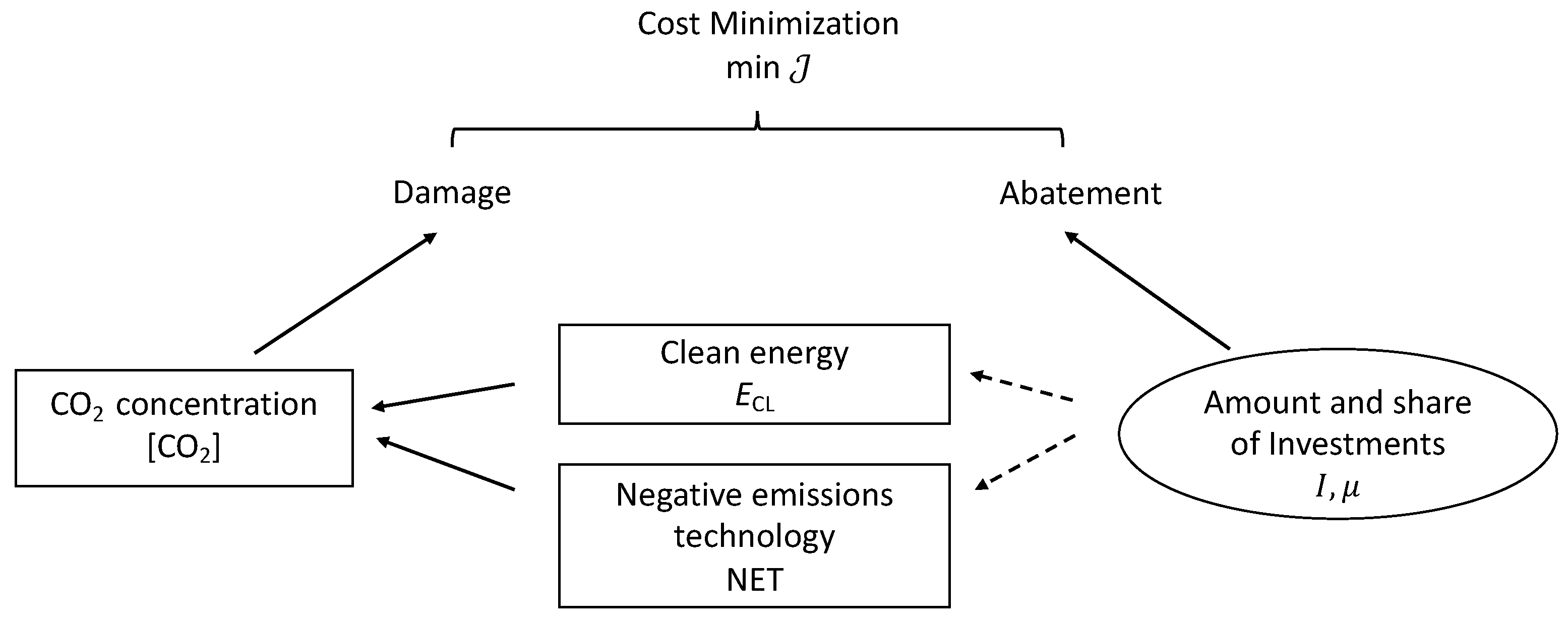
In this study, we developed a mathematical model that captures the essential features of the coupled economic–climate system; it includes the rise in CO concentrations caused by the use of emitting energy sources, as well as the mitigation provided by renewable energy and negative-emissions technologies that remove carbon from the atmosphere [26,27]. This minimalist, global mitigation model (see Figure 1) is controlled by the amount of investments allocated to emissions abatement and it enables us to explore the pathways that best combine the mitigation alternatives and distribute the economic investment while minimizing both the emissions and abatement costs. The resulting framework offers a quantitative tool to optimally allocate financial resources and help assess the key controls in the dynamics of the energy transition to inform policy decisions. Unlike previous analyses that only explored a discrete subset of options, our variational approach using optimal control theory allows us to consider the entire continuum of protocol options as a function of the global targets and for different temporal horizons. This enables us to answer the questions: what are the best strategies to counteract the CO rise, considering the limitations that the market might impose on the development of mitigation alternatives? How should investments be allocated dynamically, and in what time frame? The paper is organized as follows: Section 2 introduces the model and the coupled climate–economy dynamics. Section 3 characterizes and solves the optimal control model. In Section 4, we present the solution and discuss the optimal paths. Finally, we summarize our results in Section 5.
2. Model
2.1. Energy Demand: Fossil Fuels vs. Clean Energy
In the development of our model, meeting the energy demand is considered a crucial constraint in any mitigation scenario. This is done to avoid energy poverty, insecurity [28], and more complex scenarios, related to the fact that, on the one hand, this demand is currently only partially met, while on the other hand, it should decrease to avoid the worst climate impacts. Accordingly, we assume a given energy demand, , which has to be met by either fossil fuel energy or clean energy ,
where inequality allows for energy surpluses but not for shortages. We assume that clean energy encompasses solar, wind, nuclear, and hydropower, considering that they do not emit carbon. For simplicity, emissions related to the construction phase of clean technologies (e.g., solar panel glass melting, concrete emissions from dam buildings, etc.) are assumed to be a negligible portion of the total emissions, but can be easily accounted for by reducing the clean energy terms. In this first analysis, to keep the number of parameters low, the energy demand is considered constant. This assumption, however, can be easily relaxed to include the growing demand [28] or seasonal fluctuations, due, for example, to differences in the winter/summer demand and availability [29].
2.2. Energy Constraints and Irreducible Fossil Fuel Share
Renewables are unlikely to completely replace fossil fuels any time soon. This is the case for aviation transport as well as for the construction and deployment of clean energy technology itself [19,30]. Moreover, clean energy growth can be halted for socioeconomic reasons, which could prevent an adequate market penetration of renewables to meet global targets [31].
To account for this ‘irreducible’ fossil fuel energy demand, we place a constraint on clean energy production, as follows:
where is the irreducible part of fossil fuel energy. In the presence of this constraint (), clean energy alone cannot mitigate the climate problem [32], which then requires artificial carbon sinks.
2.3. CO Budget
The impact of climate change on human activities is usually evaluated through the concentration of greenhouse gases; here, for simplicity, it is represented by CO (this simplification can be relaxed in future analyses without altering the main model’s framework). This follows a common procedure in the literature, justified by the fact that CO is responsible for 80% of current emissions [33]; moreover, non-CO emissions are globally correlated with CO emissions, not only because they have common sources [33], but also because policies often address GHGs indistinctly.
We consider a simplified CO budget represented by anthropogenic emissions (EMI) and other natural sinks and sources (NAT) from oceans and land [34]; for simplicity, we neglect short-term effects due to rock weathering or volcanic activity (although these can be incorporated in the model if known from other studies). Additionally, an offset term (NETs) will represent the effects of natural and artificial negative-emissions technologies for carbon mitigation. With these stipulations, the global CO budget, in a well-mixed atmosphere, can be written schematically, as follows:
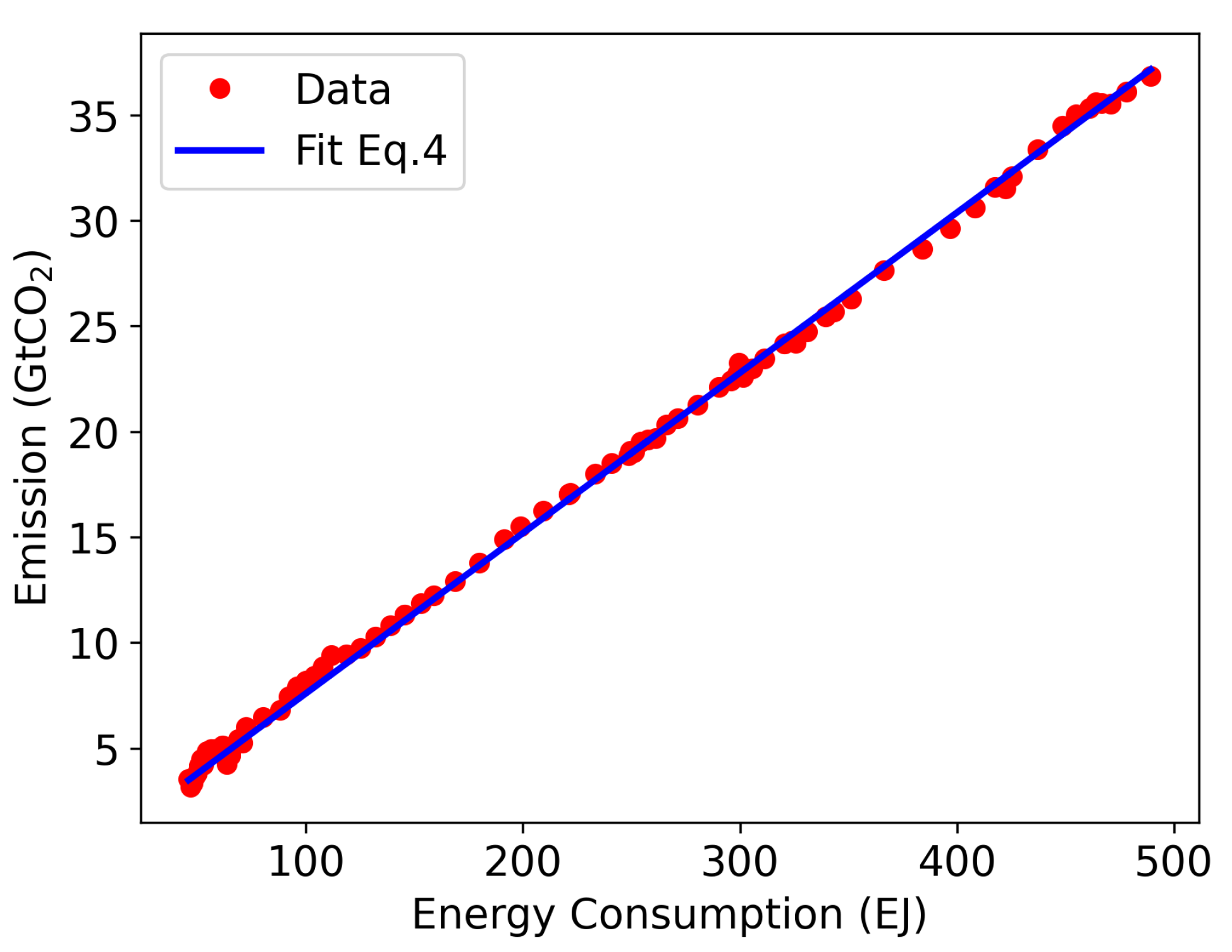
The emission rate of CO is simply assumed to increase linearly with the rate of fossil fuel use
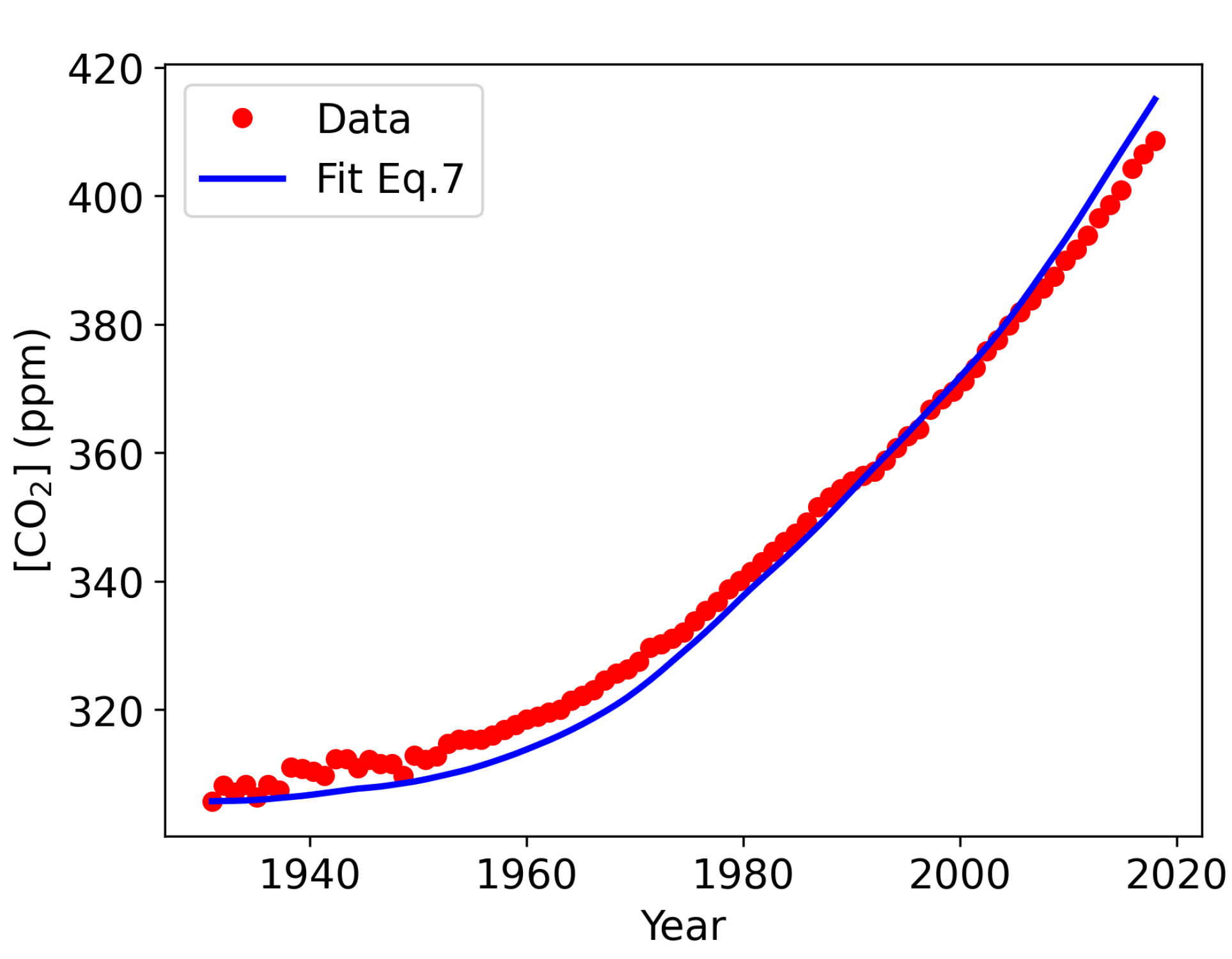
where represents the emissions per unit of energy produced from fossil fuels. Regarding the natural sinks and sources (NAT), it is estimated that only 40% of total fossil fuel and land-use change emissions remain in the atmosphere, with oceans and land absorbing the rest in almost equal percentages [35]. Based on the fact that both ocean and land sinks have been enhanced following the increase in atmospheric concentrations [35,36], the sink term is assumed to be proportional to the increased CO concentration since the pre-industrial times
where is the pre-industrial CO concentration set equal to 280 ppm [37]. For simplicity, we will start with an assumption of linearity (), although it is possible that higher CO concentrations may trigger nonlinear feedback. For example, both photosynthesis and respiration are expected to be affected at high levels of CO, with a consequent reduction of the net carbon sink [38], while the vegetation may saturate because of nutrients and water limitations, potentially making the sink sublinear. Conversely, some regions, such as those affected by permafrost melting or forest fires, may become strong sources and, thus, produce superlinear effects [39,40]. The impacts of such nonlinear effects will be considered in future contributions.
The offset term accounts for different alternatives, referred to as carbon dioxide removal technologies or negative-emissions technologies (NETs), that directly remove carbon dioxide from the atmosphere. These include carbon capture and storage (CCS), land-based climate solutions (LCS), and direct air capture (DAC). In particular, NETs have increasingly drawn attention as complementary decarbonization strategies, as it became clear that it will be virtually impossible to meet the 1.5° target without them [17,41] (in 2015, the IEA estimated that about 100 gigatons of previously emitted CO should be stored before 2050). CCS technologies capture CO at the source of production, preventing its release, and then transport and store it in suitable underground geological formations [42]. Among these techniques, the combined use of bioenergy and carbon capture and storage (BECCS) is garnering the most relevance in many mitigation scenario projections [43]. Finally, land-based solutions include forestry activities, such as reforestation and afforestation, as well as more sustainable agricultural practices aimed at storing more carbon [44,45,46]. Other promising yet less explored alternatives include enhanced weathering, as well as ocean-based measures, such as ocean alkalinization and ocean iron fertilization [47,48,49]. If NETs appear promising, it should be noted that their implementation is far from imminent, as they are still under scientific scrutiny regarding concerns for leakage of storage units and risk of reversed sinks; moreover, the implementation costs are still high and public awareness and acceptance of NETs are low [42]. Regardless of these issues, in our minimalist description, we will not distinguish among NETs and group them in an offset rate collectively indicated as NET (e.g., GtCO/yr),
In summary, incorporating the energy constraints and the above assumptions, the CO balance equation is
where converts from GtCO to ppm, is the emission rate per unit of emitting energy, and is the efficiency of the natural sink. In the current conditions, both and , so that overcomes NS and is increasing. The time to net zero, , can be formally defined as the time in which inputs and outputs balance in (7),
at which point the CO concentration is .
To conclude this section, it is important to stress that the present CO balance is a highly simplified caricature of reality, aimed at capturing only the main trends of the processes underlying the sources and sinks. This means that the possible lags between the emission and the actual change in concentration cannot be captured by the model [50]. Despite these simplifications, the model allows us to focus on mitigation scenarios based on a plausible and first-order response. More complex Earth-systems models with possible bifurcations and tipping points [51] could be coupled to the present framework, which would, of course, be of great interest, especially for long-term assessments.
2.4. Economics of the Energy Transition: Investments and Technological Growth
To characterize the dynamics of the energy transition, we follow an approach that is typical of economic modeling, where the investments determine the stock of a certain capital [52]. In the present case, the capital is embodied by clean energy and negative emissions technology, and its development is bound by the amount of investment devoted to the scope of the net-zero transition. According to this view, a ‘clean energy capital’ and a ‘negative emission technology capital’ are assumed to accumulate thanks to the total annual investment . As the mitigation effort is enabled by the development of different transition technologies, the total funding for each mitigation technology needs to be allocated wisely. Thus, to account for the way the model allocates funding, we adopt an investment share attributed to clean energy production, indicated as , and varying between 0 and 1. The complement, , is allocated to the negative emissions technology development. We also assume that the investments are followed by immediate production, which means that if a certain share (or ) is allocated for clean energy (or NET), this translates to newly installed clean energy (or NET) capital according to a market efficiency . Each energy technology undergoes depreciation, on account of its degradation over time and the need for maintenance. The depreciation factor, denoted as , reflects the rate at which the technology loses value. In our model, we assign a conservative estimate for the average lifespan of these technologies, which is approximately 30 years (e.g., solar panels or wind turbines). This corresponds to a depreciation factor of approximately . With these assumptions, the evolution of clean energy and NET potential is given by
respectively. Clean energy technology is currently much more developed compared to removal technologies, owing to decades of advances in research, production, and implementation. As a result, the same amount of investment translates to different outcomes when one compares clean energy and offsets. To account for such a disparity in the current conditions, we assume that , meaning that clean energy potential is higher per unit investment compared to negative-emissions technologies. Further development of removal technologies and consequent market penetration may change this situation and this ‘learning process’ may be easily included in future model extensions. Temporal variability in such market efficiencies could also be due to market temporal variability as well as fluctuations in clean energy production due, for example, to solar intermittency [53].
3. Optimal Control Problem
Among the virtually infinite multitude of possible scenarios, the optimal path for the best allocation of resources, leading to a rapid transition, without placing an excessive burden on society, can be determined as an optimal control problem. Rather than finding multiple alternative strategies that compromise between conflicting interests, we focus on identifying a single optimal alternative that aggregates all the objectives in one [54]. This is achieved by minimizing a suitable cost function, as described in the next section, using the methods provided by Pontryagin’s maximum principle (more details are provided in the next section). This approach is similar, in this respect, to the method used in the DICE model [21,23], which also employed an optimization framework in a global approach to climate change.
3.1. Cost Function
When considering a mitigation effort, the costs to be weighted are related to the damages caused by sustained emissions and the implementation of abatement strategies. Formally, the total cost is expressed as
the various terms are discussed in what follows.
Quantifying the economic risk and damage from climate change obviously entails a great deal of speculation. In general, the cost of climate change refers to a broad range of related biophysical, environmental, social, and economic issues [55]. Usually, a damage function is used to estimate the economic cost of higher levels of CO, relative to a baseline corresponding to the pre-industrial CO level. Different forms of this function have been proposed in the literature, in spite of the difficulties in making a confident assessment of the climate change impact on the economy [55,56], as well as in calibrating it, especially when it comes to estimating impacts related to health and the environment [57].
The so-called social cost of carbon (SCC) has been advocated as an effective and comprehensive concept when evaluating the growing emissions threat [23]. The SCC is defined as a ‘monetary estimate of the climate change damages to society over time from an additional tonne of carbon dioxide, including market impacts such as agricultural productivity, energy costs and infrastructure damage as well as impacts on non-marketed goods such as ecosystems and human health’ [55]. Its adoption stems from the preferred use in policy. The Biden administration has raised it back to USD 51 [58] and others recommend an increase beyond USD 200 [59]. Thus, we conveniently use the SCC to link the damage term proportionally to the cumulative emissions since pre-industrial times [60]
The damage is assumed to be zero once the CO concentration decreases to the pre-industrial level. For the sake of simplicity, we neither consider CO concentrations lower than the pre-industrial level, nor the nonlinear damage function of CO concentrations. These extensions will be considered in future contributions.
In general, the abatement cost is the cost to reduce or prevent pollution following a new regulation [61]. Here, it includes the investments devolved to the development of mitigation technologies and their installation. Clean energy and NETs, being “physical capitals”, cannot be built instantaneously but need to be installed in order to produce. To capture this inertia in the capital accumulation process, we account for adjustment costs on the investments, which are often overlooked in the literature [55]. This means that each unit invested translates into less than a unit of clean energy or NET, or, equivalently, in an additional cost per unit invested, as a consequence of the market rigidity [62,63]. In the literature, the growth rate of renewables is often constrained by a maximum value based on previous development [64]. Here, we do not preclude higher and faster development if investments are mobilized, and we attribute the role of slowing down growth to adjustment costs.
Thus, the abatement consists of two terms—an investment and an adjustment cost—where the latter is quadratic in investments I, implying that the speed at which the economy decarbonizes is relevant for the cumulative cost [12]. Adjustment costs may also reflect public resistance to renewables and removal technologies. Social acceptance poses a significant challenge for renewables [65,66,67]. The risk of delays in installation and operation often arises from public resistance, which can outweigh technological considerations, although the extent may vary depending on the type and scale of the installation [68]. By inserting the functional forms corresponding to the previous considerations, the cost function becomes
where the abatement costs relative to clean energy and offset evolution are distinguished, each one partitioned according to the share coefficient ( or ) and their own calibration coefficient ( or ) for adjustment costs. Previous studies [12] estimated an adjustment cost coefficient of for renewable energy. However, when it comes to carbon removal technologies, there is a lack of specific estimates due to their limited penetration in the market. Given the nascent stage of their expansion, we conservatively assume that their adjustment cost coefficient needs to be at least three times higher. Therefore, we consider an adjustment cost coefficient of for carbon removal technologies.
It is worth highlighting that our optimization approach revolves around a single objective function that encompasses multiple terms. Alternatively, one could choose to separate these terms and optimize them individually within a multi-objective framework. Here, a single objective function directly yields the optimal compromise solution among the different terms, which have already been expressed in monetary values. Adopting a multi-objective approach would result in a range of options, necessitating a decision rule to select a solution based on preferences concerning damage costs or mitigation costs. Incorporating policymaker preferences is beyond the scope of this study, as our primary focus lies in exploring the best solution and its evolution over time.
3.2. Intertemporal Optimization
The optimization is stipulated to take place over a finite planning horizon . A short planning horizon prioritizes the near-term utility but ignores events past the horizon, while a longer horizon demands more planning effort but entails better foresight. During this period , the cost is determined by the co-evolution of emissions, clean energy, and NETs, according to the Equations (7) and (9). Additionally, the cost is discounted for future times to project the lower importance of all future costs to the present time of optimization. As a result, the cumulative cost over the entire planning period is expressed by the functional
where is the discount rate.
The investment and the clean energy share are considered the knobs with which we can control the cost to adjust the decarbonization path. As a consequence, for the optimal solution, the functional has to be minimized over all the possible realizations of the control variables of the system, and ,
To ensure physically meaningful controls, the control variable is constrained to the domain , the so-called admissible control set. Note that the carbon price itself (i.e., SCC) could have been used as an alternate control variable, as it is often used in evaluating alternatives in the literature. Here, we considered it more meaningful to have the carbon price to be imposed exogenously so that the effect of its variation on the optimal investments is analyzed.
3.3. Application of the Maximum Principle
We follow an optimization based on the application of the Pontryagin maximum principle [69]. The first step consists in writing the associated Hamiltonian as the sum of the cost functional (12) and all constraints on the three state variables . Formally, this corresponds to writing
where represent the co-state variables of the optimization problem or Lagrange multipliers. The multiplier is associated with the state-variable constraint (2), which only becomes active once reaches , and then prevents it to exceed when the equality condition is met (see [70], p. 301), i.e.,
The application of the Pontryagin maximum principle provides the first-order conditions for the optimal control problem. These include the adjoint equations satisfied by the time-varying Lagrange multipliers,
and the equations for the control variables
From (18), the expression for I and can be derived in terms of state and co-state variables. We discard the solution for zero investments, , which represents the no-mitigation business-as-usual scenario, and focus on the other solution, which entails
where is the following discontinuous function
which enforces the constraint (2). It can be shown that the problem is well-defined for minimization since the second derivative of the Hamiltonian is positive in the control variables (convex optimization). Incorporating the limits on the control variables given by their feasible values, , allows us to find the expression for the optimal control pair
Substituting expressions (19) and (21) into Equations (7), (9), and (17) yields a system of 6 ordinary differential equations in the 6 variables, , , , . In order to solve it, additional initial conditions on the state variables and the boundary conditions for the co-state variables (the transversality conditions) must be provided. We take the initial clean energy capital to be the energy consumption (EJ) generated from renewables in 2021 [8]. As for the current deployment of NETs, it is considered to be negligible, leading us to set . The state variables , , and are free to take any value at their final time so the system is closed by imposing [70]. A numerical solution is employed to track the system’s evolution. All the parameters used for the numerical solution are listed in Table A1 in Appendix A. The optimization solution provides the co-evolution of the six variables over time by selecting the optimal values for I and to minimize the total cost. The obtained profiles are discussed in the following section.
4. Results and Discussion
4.1. Optimal Strategies
The solution of the system described in the previous section provides an optimal way to achieve a reduction in emissions by managing investments, in terms of both their intensity and share between net emission technologies and clean energy.
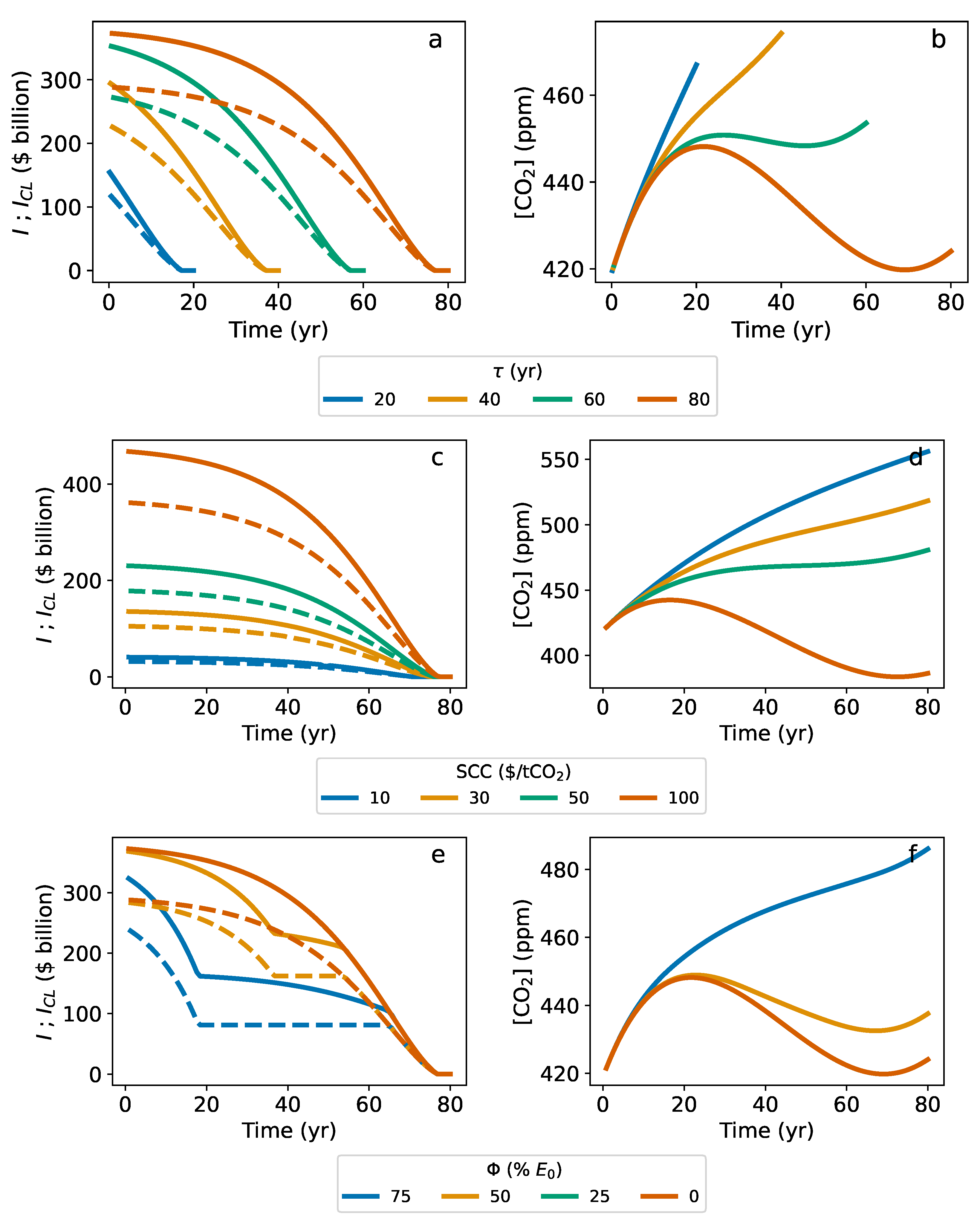
The number of investments and the total cost crucially depend on the time span of the mitigation strategy. A short planning horizon implies very low investments. As shown in Figure 2a,b by the curves for the 20- and 40-year investment plans, the inability to account for higher damage costs, which characterize longer time spans, affects the cost minimization and favors inaction, i.e., low investments. The reason for this is that the foreseeable damage for those short time spans is not enough to motivate an investment flow towards the abatement effort, which is then kept low by cost minimization. The annual investments increase with longer planning horizons. The mitigation is promoted in the early stages of the planning, to avoid a prolonged CO increase and attenuate the burden of environmental damage on the abatement effort. As shown by the dashed lines in Figure 2, the largest share of the investments is allocated to clean energy.
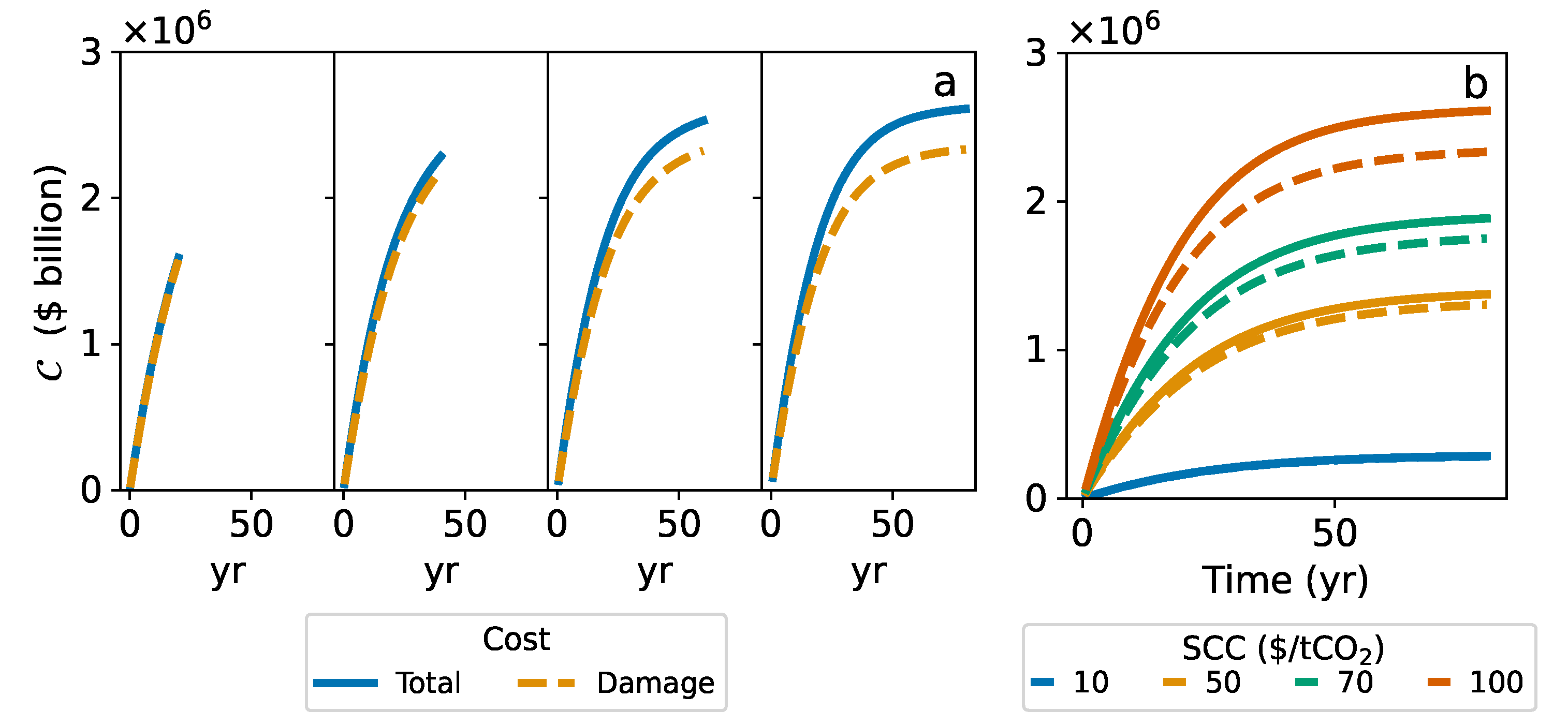
Figure 2b shows the CO concentration corresponding to the optimal investment profiles. As expected, a small investment implies an almost undisturbed growth of CO concentration. As the foresight improves, more abatement becomes possible and the CO curves are then lowered. The cumulative cost for each plan is reported in Figure 3a. For short-term horizons, the cost is fully attributable to environmental damage (orange dashed lines) because of the negligible mitigation effort. The total cost obviously increases with the horizon time, but the percentage due to environmental damage decreases with longer-term planning.
The role of the SCC is analyzed in Figure 2c,d, which shows how the weight given to the carbon-related damage is also crucial in determining the optimal path. A poor estimate of the damages due to CO greatly affects the mitigation policy. As depicted by the different trajectories in Figure 2c,d, the value given to the SCC determines the proportion of the mitigation. For low SCC, the damage costs are lightly weighted in the minimization and this hinders the mitigation effort. As a result, in such a case, the optimal trajectory is characterized by low investments and CO levels rise (blue and yellow lines). The total cost is almost entirely due to environmental damage (dashed lines in Figure 3b). Increasing SCC places a higher weight on damage, thus giving higher priority to abatement. Hence, investments are higher, as shown by the green and orange lines in Figure 2, and, as a result, CO concentrations are reduced. In this case, investments are promoted at the early stages of planning, causing an early steeper cost increase compared to plans with negligible mitigation (Figure 3b). A higher share of the cumulative costs is devoted to abatement, and the environmental damage for these scenarios is lower (dashed lines). Increasing SCC also has an impact on the temporal distribution of investments. A higher SCC implies more effort to lower emissions; because of the limit on clean energy demand, Equation (2), it is advantageous to widen the share allocated to negative-emissions technologies despite the higher costs, which explains the higher total costs observed in the same time span (Figure 3b).
The results of the optimization also show that, in general, the investments are preferably directed towards clean energy (dashed lines in Figure 2a,c,e). The higher share towards clean energy is explained by the higher cost-effectiveness compared to negative-emissions technologies (NETs). To explore different clean energy scenarios, the optimization was performed, constraining clean energy production to 100, 75, 50, 25% of the total energy demand (i.e., , respectively). As shown by the investment profiles in Figure 2e,f, clean energy is prioritized over the whole time plan. Investments are high during the early stages of the optimization, and the development of clean energy technology rapidly reaches the 25% and 50% caps (respectively, blue and yellow curves). Once the maximum renewable energy capacity is reached, the only abatement possible is related to negative-emissions technologies, but because of their high cost, the damage is preferred. As a result, when the clean energy production limit is reached, there is an abrupt change in the investment profile, as the share in the investment in clean energy drops in favor of NET, and only a small investment is allocated to the maintenance of the clean energy capital established thus far. The lower the limit on clean production, the earliest this change in investment profile occurs (green and orange curves overlap in Figure 2e). With the deployment of large investments at the beginning (see Figure 2e), net-zero emissions are reached quickly: Figure 2f shows the rapid decay of emission rates in response to the fast development of clean energy, ultimately reaching zero emission rates in less than 20 years. However, when clean energy production is too heavily constrained, the CO concentration cannot be efficiently reduced even with large financing. The limiting factor is the ‘irreducible’ fossil fuel amount that is allowed to stay in the energy picture: the scenario with (red line in Figure 2f) never reaches net zero.
4.2. Need for Rapid Investments
The optimal profiles obtained clearly show the necessity of rapid and large investments. A similar conclusion was previously reached by [71,72,73]. In particular, the fast deployment of resources enables the quick development of clean energy production, avoiding further CO increases for prolonged fossil fuel use. Eventually, the sum of the investments decreases in time towards the end of the planning horizon, but the biggest benefits are obtained by allocating most of the financial resources early on. The massive increase in investments in the energy sector is not surprising [74], but in practice, poses a huge challenge. Progress in a sustainable energy transition requires aggressive and well-financed research as well as major resource transfer from developed economies [5]. These efforts also require the support offered by confidence in the development of a large-scale market for renewables [60]. Examples of successful implementation of such investment can be found in several European countries that have pioneered policies promoting investments in renewables [75,76]. Denmark, for instance, began its transition to renewable energy as early as the 1980s. Similarly, countries such as Sweden, Iceland, Germany, and Spain have demonstrated the effectiveness of early resource allocation in achieving successful and economically beneficial carbon mitigation. Furthermore, more recent efforts in countries across Latin America have also shown promising results in renewable energy adoption. Notably, many European countries have surpassed their renewable share of primary energy targets for 2020. Assessments have been made regarding the positive impacts on the economy, such as enhanced energy security, increased employment rates, and technological advancements, emphasizing that considerations beyond mere profit have been taken into account.
4.3. The Reward of the Farsighted
The SCC assigns a certain weight to environmental damage, reflecting a higher or lower concern for climate change impacts. A low SCC denotes scarce concern for future damage; in this case, the cost minimization concludes that the abatement is too costly and suppresses it. On the contrary, a high SCC reflects a pessimistic view of future damage and, accordingly, it weighs it heavily.
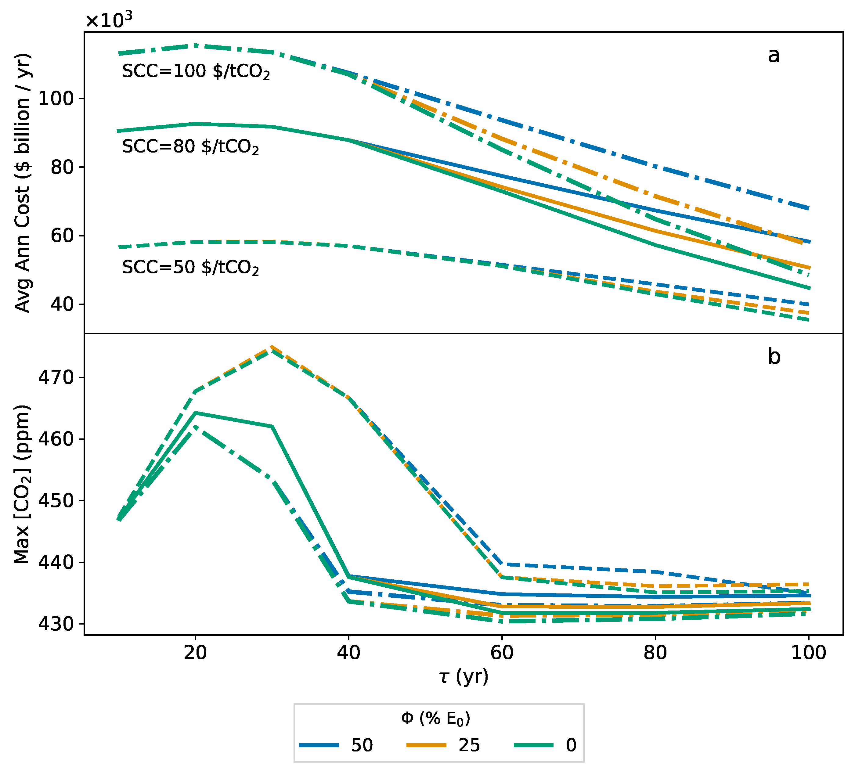
The annual cost of optimal plans for different SCC values and planning horizons is compared in Figure 4a. Increasing the SCC produces different effects, depending on short- or long-term horizons: in the short term, a higher SCC implies higher annual costs and, therefore, as noted before, short-term inaction is favored. CO concentrations peak over 460 ppm, far above the threshold of 450 ppm, for which ‘dangerous climate consequences’ are expected [77]. With this, the cost is fully due to environmental damage, which in turn is proportional to the SCC. Raising the SCC increases the average annual cost, as expected, as an investment in mitigation is promoted. Abatement takes a higher percentage of the cumulative cost but efficiently cuts the level of maximum CO concentration reached (panel b in Figure 4). By assigning greater damage from carbon concentration rise, we can avoid reaching threatening environmental conditions, and the SCC does not have to be dramatically high to meet these conditions. While it may be problematic and costly to swiftly spin large investments, the cost is, nevertheless, inferior to waiting.
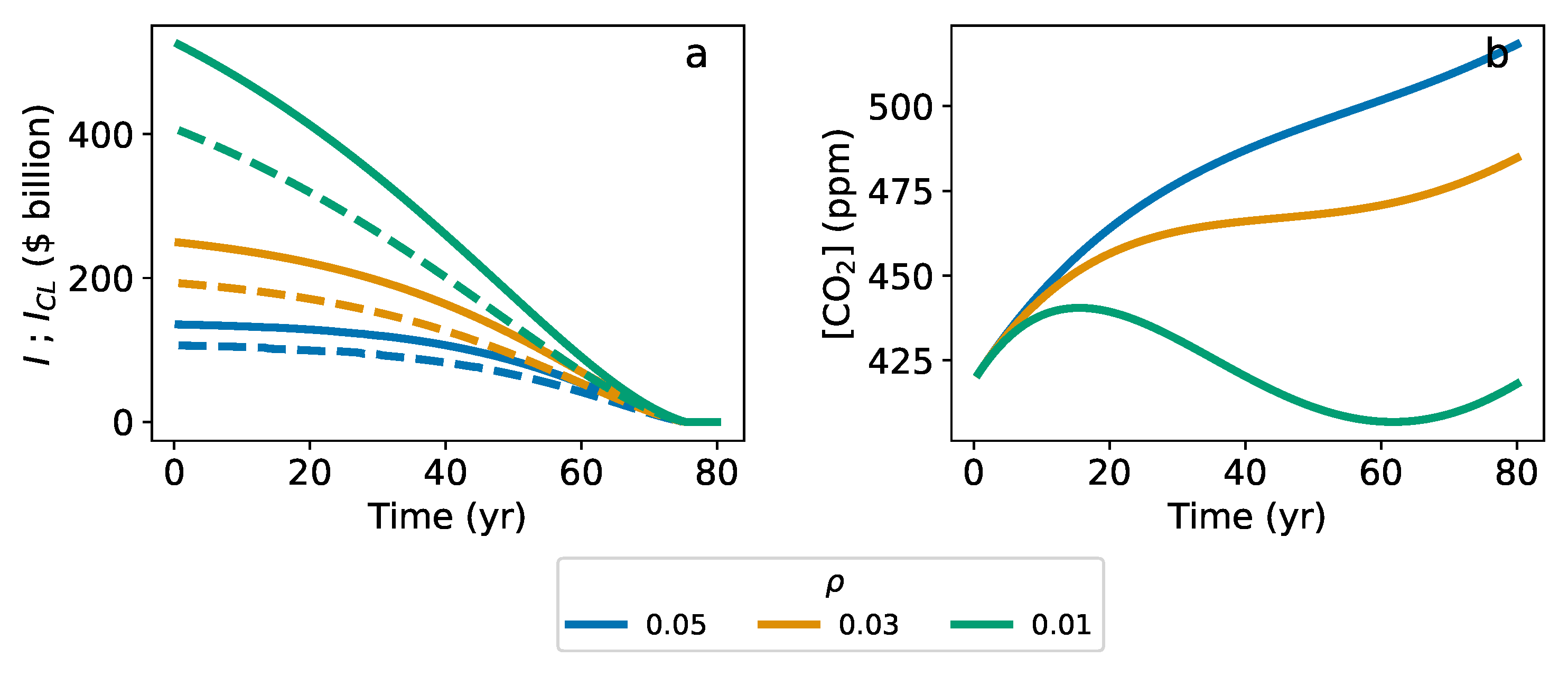
For cost optimization, the discount rate is essential to consider future welfare in long-term analysis, such as climate mitigation strategies. A previous study assessed that a reduction in the discount factor by even a few percentage points will double the current social cost of carbon [78]. It is common practice to use a discount factor of approximately 5%. However, to assess the impact of intertemporal discounting on the results, we conducted additional analyses using lower discount rates of 3% and 1%. As shown, a lower discount rate would encourage a more short-term effort, leading to a substantial improvement in abatement impacts. Comparing the green and the orange curves in Figure 5, one can notice that a difference of only a couple of percentage points in the discounting can determine whether to invest or not in abatement, with huge consequences on CO concentrations.
4.4. Urgency of Clean Energy Expansion
As discussed before, a myopic view of the potential damage from CO hardly justifies a massive resource deployment for mitigation. For horizon spans of less than 40 years, the costs of mitigation are too high, and avoiding action appears to be the most cost-effective approach. Since in this case there is no interest in developing clean energy and negative emissions technology, the constraint on clean energy production does not really matter. For short-term planning, the annual cost is the same regardless of the fossil fuel policy, as it is overwhelmingly due to environmental costs, which rise linearly with CO. The critical planning horizon for which abatement begins to matter depends on the SCC. The lower the SCC, the longer is convenient to wait from an economic point of view. As shown in Figure 4a, the averaged annual costs start decreasing only after about 60 years for an SCC equal to 50 $/tCO, as soon as the short-term inaction is not optimal anymore and a proper abatement effort is promoted. For SCC values of 80 and 100 $/tCO, mitigation incentives start in 50 and 40 years, respectively. Opting for substantial fossil fuel use results in the highest cost in the long term. In the case in which clean energy only covers 50% of the total energy demand, the mitigation effort does not pay off. CO still increases with consequent damages and high costs. As shown in Figure 4a, imposing a constraint on clean energy production at half of the total demand leads to higher annual costs compared to less constrained pathways (orange and green curves in Figure 4), because of the limited ability to sufficiently reduce emissions. In the long term, the action is cost-effective and early investments prevent further CO increase, thus preventing subsequent environmental costs. The different curves in Figure 4 show how the annual cost decreases for pathways that allow for more clean energy (lower ). Investment costs for mitigation contribute to raising the annual costs in short-term planning; however, with a longer horizon, they descend below the annual costs associated with short-horizon low-mitigation plans. After about 60 years, the benefits of early-stage investments become apparent. After this time, the cost-effectiveness depends on the limit put on clean energy production (or the policy adopted). Replacing a larger proportion of fossil fuel energy with clean energy, as depicted in the 0% irreducible fossil fuel path in Figure 4, offers significant long-term benefits. The support and promotion of renewables, which are already cost-competitive in the short term, prove to be more effective in achieving emission reductions over the long term.
This observation aligns with findings from previous studies [26,79] and is exemplified by countries such as Sweden and Germany, where early investments have facilitated a rapid expansion of renewable energy capacity. These countries have experienced consistent reductions in emissions and reduced the dependence on fossil fuels, while also generating economic revenue and reaping co-benefits, such as employment opportunities. The advantages of early investments in renewables have contributed to mitigating the overall costs of transitioning to clean energy sources. However, it is important to acknowledge the challenges associated with the market penetration of renewables in economies that have long relied on fossil fuels. Despite these challenges, increasing the contribution of clean energy significantly reduces annual costs, which can be lower than the costs of inaction and future damages, as highlighted in previous research [80].
4.5. The Uncertain Potential of NET
To gain a comprehensive understanding of the potential role of NETs in achieving carbon mitigation targets, it is crucial to consider the uncertainties associated with their costs and deployment. Efforts have been made to estimate the actual costs of implementing NET; Fuss et al. conducted important work to provide a constrained range for each technology, considering the average cost per tonne of carbon removed [41]. However, the lack of large-scale implementation hampers accurate predictions of future expenditures and the potential cost reductions that may occur, similar to what has been witnessed in the renewable energy sector.
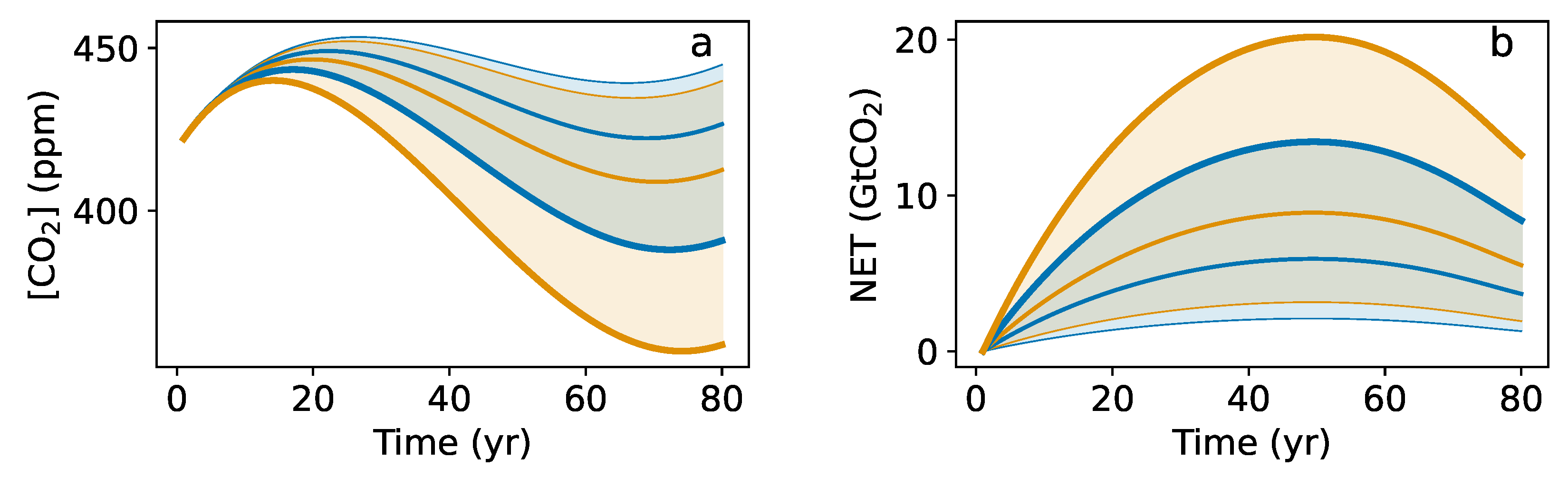
To explore these uncertainties, we consider scenarios that assume a lower average cost for NET implementation. This could be attributed to factors such as “learning by doing”, leading to natural cost decreases as the technology matures, or the preference for deploying cheaper NET options over more expensive ones. For example, afforestation, being one of the least expensive NET options, could play a significant role in the overall carbon removal effort. Similar to renewables, the prospects of NETs can vary significantly in the real-world context. To account for this uncertainty, we examine three cost estimates (200, 300, and 500 $/tCO) to create a range of scenarios, allowing us to analyze how changes in NET costs affect investment distribution. We explore the sensitivity of investment allocation and CO pathways to different cost scenarios. Additionally, we repeat the analysis using the same cost ranges but with a lower value of the adjustment cost coefficient , simulating a smoother market penetration similar to what occurred with renewables (yellow range in Figure 6). In the plotted curves, the thinnest curve represents the highest NET cost scenarios for both (blue range) and (yellow range). As expected, the CO concentration remains high since the NETs are not cost-effective in this scenario and their deployment is limited. The mid-cost scenario demonstrates greater effectiveness in mitigating the rise in CO concentrations. The deployment of NETs over time aligns with most estimates within a range of 0.5–5 Gt CO yr of carbon dioxide removal by 2050 [41,81]. With even lower costs per tonne of carbon removed, the deployment over time increases due to enhanced cost-effectiveness. The estimated profiles come closer to the necessary deployment levels required to stay on the 1.5 °C scenario.
Our analysis reveals the considerable uncertainty surrounding the costs and potential of NET. The wide range of cost estimates poses challenges to the widespread adoption of NET, as a broader cost range may favor more economically favorable technologies such as renewables. However, in cases where deployment limitations are overcome, NET could play an equally significant role in carbon mitigation efforts, demanding a higher share of investment for their expansion. It is crucial to consider sector dependencies as well, where specific NETs could enable certain sectors to surpass their irreducible fossil fuel share [82]. On the other hand, the continuously declining costs of renewables may overshadow the potential offered by NET.
4.6. Higher Mitigation Budget Decreases the Total Cost
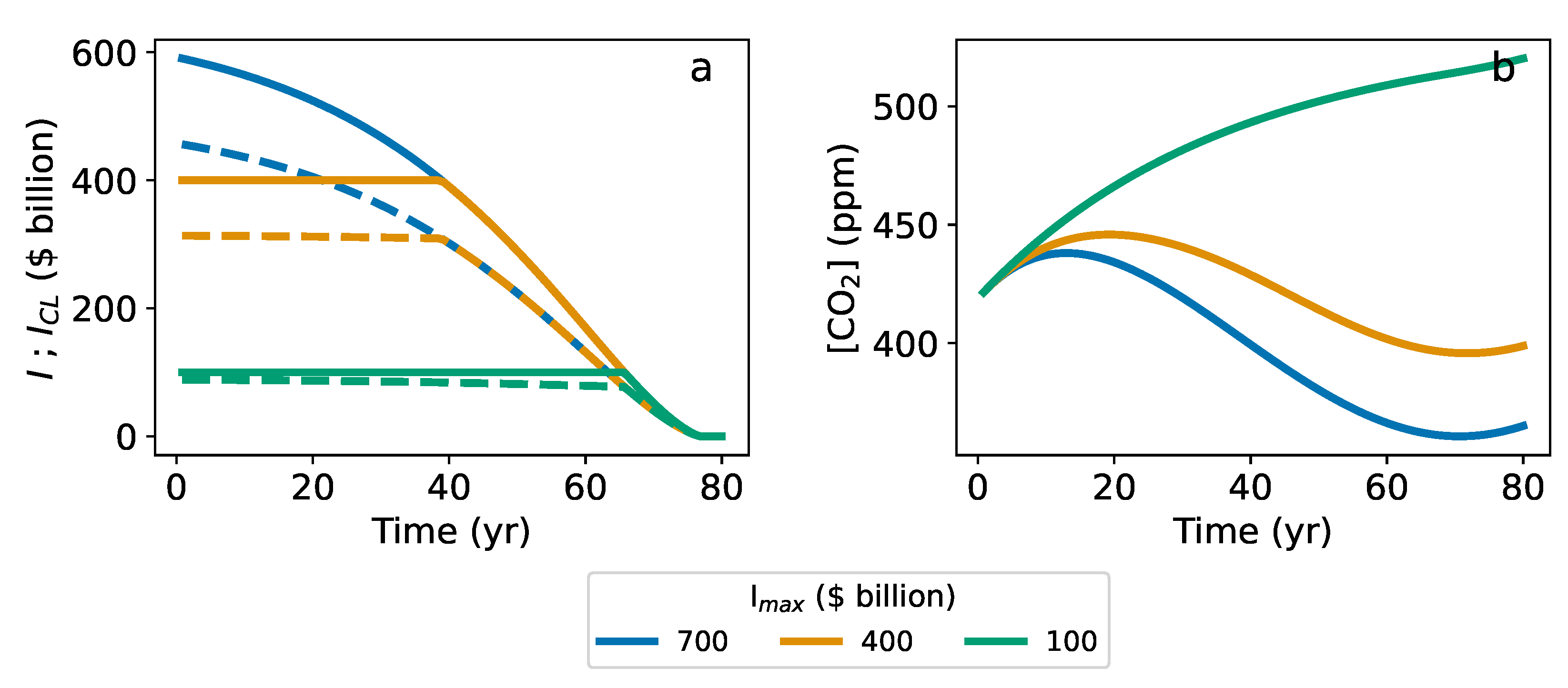
So far, we considered the mitigation effort to be free of constraints, other than satisfying the optimal cost condition. It is interesting to look at how the mitigation strategies adapt when the financial resources to be allocated for the abatement are limited. For this, we also consider the case in which the annual investment cannot exceed a certain threshold (see Equation (21)), which can reflect the expendable budget elected by governments. One key advantage of the model is its flexibility in accommodating specific budget allocations for mitigation by individual countries. This allows for the adjustment of constraints within the model to accurately reflect the financial resources allocated by a particular country towards their mitigation efforts. The effect of such a limit on investments deeply affects the evolution of CO. Figure 7 compares the mitigation paths in different budget limits (USD 700, 400, 100 billion/year). In the presence of this cap on investment, Figure 7a shows that the optimal investment is constant for most of the planning horizon and is equivalent to the maximum value allowed. This means that the best strategy is to allocate the whole available budget. However, even following this choice, the mitigation impact is considerably delayed in the case of a high budget, or, in a low budget case, completely inadequate to counteract the carbon dioxide increase.
The effect of a limited budget for abatement investment on the technological development of clean alternatives is twofold. First, the limited budget breaks clean energy development. For the high-budget case, the development is delayed but manages to reach the same level of development as in the unlimited budget case. This strategy carries a good mitigation impact at the end of the planning horizon. If the budget is set too low, then the clean energy development is not only delayed but also cannot reach the stage necessary to mitigate successfully in the horizon’s time span. The CO rises almost uncontrolled. This scenario exemplifies the real-world experiences of countries such as Sweden, where a higher investment in clean energy expansion has enabled successful mitigation efforts. On the other hand, countries that have fallen behind their carbon targets can attribute their challenges to the limited investment allocated.
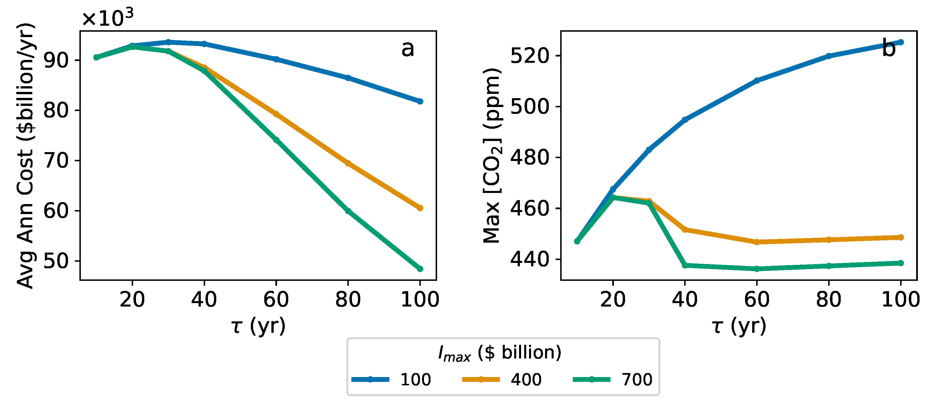
The second impact concerns the role given to negative emission strategies. In Figure 7a, the optimal profiles show the total investment being basically equal to the clean energy investment in the lowest budget scenario (green curve). A limited budget imposes the optimal choice of not investing at all in carbon removal strategies. The higher cost prevents a fruitful allocation of investments there, so the NET development has a minimal contribution only at later stages in the strategy. In the short term, putting a limit on investments does not affect the resource allocation choice; for short-term horizons, investing in mitigation appears purposeless and budget limits do not matter. This is the reason why the annual cost of mitigation is not affected by the budget limit, as shown in Figure 8a for short-term horizons. On the contrary, for longer-term horizons, it becomes optimal to invest in mitigation and counteract the damage cost, so that the total cost sensibly decreases with a longer planning horizon.
The limits on investments cause the mitigation efforts to be less efficient, making it more challenging to counteract the damages. As shown in Figure 8b, CO concentration levels reach the maximum values for the lower budget scenario (blue curve). As a consequence, because of the contribution of damage costs, the lower the cap on investment, the higher the average annual cost. The current investment in clean transition has reached just above USD 700 billion according to the IEA [83], so in order to achieve the economic optimum while also avoiding overshooting CO concentration levels of 450 ppm, more resources should be allocated to mitigation efforts.
5. Conclusions
We used optimal control theory to determine the most effective policy to direct the economy toward decarbonization. The optimization provides the optimal profiles of the controls, identified in the amount and the redistribution of investments to be allocated for the mitigation effort. The optimal temporal pathways of investments, along with the optimal distribution of mitigation alternatives, suggest that both technological and budget constraints, as well as adjustment costs, play essential roles in the transition. In particular, the analysis of the optimal strategies demonstrates the priority of the fast development of clean energy alternatives. In practice, the price decline of wind and solar energy makes these alternatives the most competitive in terms of cost-effectiveness and calls for a strong policy action to help market penetration and investment development [12,84]. Including the cost of fossil fuel energy production, which is neglected here, would only reinforce this point.
The social cost of carbon appears to be a crucial knob in controlling the transition. When the damage function is properly set, economic optimality favors stringent abatement pathways (see also [85]). The discounting of future costs should also be reduced to favor prompter mitigation action. The role of the planning time also emerges as a determining variable, related to the fact that at the later stages of the planning, the abatement effort is inhibited. This stems from the goal of economizing the resources within the planning time so that toward the end of the horizon time there is no benefit in allocating investments to mitigate subsequent damage. From game and behavioral theory perspectives, this attitude is completely rational. However, while it is understandable to have time-limited climate targets, taking these targets to their logical consequences could result in certain forms of ‘global Ponzi schemes’ at the expense of environmental resources, justified by the illusion of exiting before the inevitable crash. As known in classical economics, Ponzi schemes are fraudulent schemes that allow for ‘optimal’ super profits in the short term, but they are characterized by a very brief time horizon before a certain market collapse [86,87,88]. Planning for longer time horizons helps to avoid such unsustainable behaviors when approaching the most sustainable long-term optimal path, i.e., the well-known turnpike property [70,89].
Several modeling assumptions could be relaxed in our modeling framework. In particular, here, the future of the coupled climate and economic evolution is assumed to be deterministic. Including high-dimensional and stochastic components in climate and economic systems is high on the priority list of extensions in this model. Introducing stochasticity would capture the inherent risks associated with climate change and market shocks, which could accelerate the need for action.
Additionally, the versatility of our model allows for customization to specific geographical and political contexts. It can be easily modified to incorporate region-specific energy demands, investment budgets, and costs for renewables and NET. This flexibility enables the exploration of scenarios in diverse contexts, offering valuable insights into the potential outcomes and effectiveness of different strategies.
Furthermore, damages are considered a linear function of emissions; nonlinear feedback in the climate–economy system would modify the optimal pathways, especially when including social components [59,67]. Exploring different forms of the damage function would also be interesting, given the well-known uncertainties [90,91], including the estimates on negative-emissions technologies [4]. These extensions will be considered in future work.
Author Contributions
Conceptualization, methodology, and investigation, S.C. and A.P.; writing—original draft, S.C.; writing—review and editing, S.C. and A.P.; funding acquisition, A.P. All authors have read and agreed to the published version of the manuscript.
Funding
This research received no external funding.
Institutional Review Board Statement
Not applicable.
Informed Consent Statement
Not applicable.
Data Availability Statement
The code for model simulation data utilizes the GEKKO Optimization Suite [92] and was deposited at https://github.com/sarceras/OptInvest.
Acknowledgments
The authors acknowledge support from the BP through the Carbon Mitigation Initiative (CMI) at Princeton University and the High Meadows Environmental Institute (HMEI).
Conflicts of Interest
The authors declare no conflict of interest.
Appendix A

Table A1.
Model parameters.
| Symbol | Unit | Value | |
|---|---|---|---|
| Energy demand | EJ | 556 a | |
| Current emissions | GtCO/yr | a | |
| Depreciation rate clean energy capital | − | 0.03 b | |
| Depreciation rate NET capital | − | 0.03 b | |
| Energy carbon efficiency | GtCO / EJ | a c f h | |
| Natural sink efficiency | - | c i | |
| Clean energy efficiency | EJ/$billion | d | |
| NET efficiency | GtCO/ $ billion | e | |
| Social cost of carbon | $billion/GtCO | ||
| Irreducible fossil fuel energy | EJ | ||
| Max annual investment | $billion | f | |
| Max clean energy investment share | - | 1 | |
| Emission concentration conversion | ppm/ GtCO | c | |
| Discount rate | - | ||
| Adjustment cost coefficient | - | g | |
| Initial level | ppm | 419 | |
| Pre-industrial level | ppm | 280 | |
| Initial level | EJ | 32 a | |
| Initial level | GtCO | f |


References
- van Soest, H.L.; den Elzen, M.G.J.; van Vuuren, D.P. Net-zero emission targets for major emitting countries consistent with the Paris Agreement. Nat. Commun. 2021, 12, 2140. [Google Scholar] [CrossRef] [PubMed]
- Scheffers, B.R.; De Meester, L.; Bridge, T.C.L.; Hoffmann, A.A.; Pandolfi, J.M.; Corlett, R.T.; Butchart, S.H.M.; Pearce-Kelly, P.; Kovacs, K.M.; Dudgeon, D.; et al. The broad footprint of climate change from genes to biomes to people. Science 2016, 354, aaf7671. [Google Scholar] [CrossRef] [PubMed]
- Dietz, S.; Hope, C.; Patmore, N. Some economics of ‘dangerous’ climate change: Reflections on the Stern Review. Glob. Environ. Chang. 2007, 17, 311–325. [Google Scholar] [CrossRef] [Green Version]
- Rogelj, J.; Schaeffer, M.; Meinshausen, M.; Knutti, R.; Alcamo, J.; Riahi, K.; Hare, W. Zero emission targets as long-term global goals for climate protection. Environ. Res. Lett. 2015, 10, 105007. [Google Scholar] [CrossRef]
- Deutch, J. Is Net Zero Carbon 2050 Possible? Joule 2020, 4, 2237–2240. [Google Scholar] [CrossRef] [PubMed]
- Tanaka, K.; O’Neill, B.C. The Paris Agreement zero-emissions goal is not always consistent with the 1.5 °C and 2 °C temperature targets. Nat. Clim. Chang. 2018, 8, 319–324. [Google Scholar] [CrossRef]
- Jewell, J.; Cherp, A. On the political feasibility of climate change mitigation pathways: Is it too late to keep warming below 1.5 °C? WIREs Clim. Chang. 2020, 11, e621. [Google Scholar] [CrossRef] [Green Version]
- BP. Statistical Review of World Energy|Energy economics|Home. 2021. Available online: https://www.bp.com/content/dam/bp/business-sites/en/global/corporate/pdfs/energy-economics/statistical-review/bp-stats-review-2022-full-report.pdf (accessed on 28 May 2023).
- Roser, M. Future Population Growth. Our World Data 2013. Available online: https://ourworldindata.org/future-population-growth (accessed on 28 May 2023).
- Jackson, R.B.; Quéré, C.L.; Andrew, R.M.; Canadell, J.G.; Korsbakken, J.I.; Liu, Z.; Peters, G.P.; Zheng, B. Global energy growth is outpacing decarbonization. Environ. Res. Lett. 2018, 13, 120401. [Google Scholar] [CrossRef]
- Hoffert, M.I.; Caldeira, K.; Jain, A.K.; Haites, E.F.; Harvey, L.D.D.; Potter, S.D.; Schlesinger, M.E.; Schneider, S.H.; Watts, R.G.; Wigley, T.M.L.; et al. Energy implications of future stabilization of atmospheric CO2 content. Nature 1998, 395, 881–884. [Google Scholar] [CrossRef]
- Rasmussen, T.N. CO2 abatement policy with learning-by-doing in renewable energy. Resour. Energy Econ. 2001, 23, 297–325. [Google Scholar] [CrossRef]
- IRENA. World Energy Transitions Outlook: 1.5 °C Pathway. Hydrog. Knowl. Cent. 2021, 312. Available online: https://www.irena.org/-/media/Files/IRENA/Agency/Publication/2021/Jun/IRENA_World_Energy_Transitions_Outlook_2021.pdf?rev=71105a4b8682418297cd220c007da1b9 (accessed on 15 March 2012).
- Walsh, B.; Ciais, P.; Janssens, I.A.; Peñuelas, J.; Riahi, K.; Rydzak, F.; van Vuuren, D.P.; Obersteiner, M. Pathways for balancing CO2 emissions and sinks. Nat. Commun. 2017, 8, 14856. [Google Scholar] [CrossRef] [Green Version]
- Rogelj, J.; den Elzen, M.; Höhne, N.; Fransen, T.; Fekete, H.; Winkler, H.; Schaeffer, R.; Sha, F.; Riahi, K.; Meinshausen, M. Paris Agreement climate proposals need a boost to keep warming well below 2 °C. Nature 2016, 534, 631–639. [Google Scholar] [CrossRef] [Green Version]
- Post, T.W. Pace of climate change shown in new report has humanity on ‘suicidal’ path, U.N. leader warns. Washington Post 2021. [Google Scholar]
- Fuss, S.; Canadell, J.G.; Ciais, P.; Jackson, R.B.; Jones, C.D.; Lyngfelt, A.; Peters, G.P.; Van Vuuren, D.P. Moving toward Net-Zero Emissions Requires New Alliances for Carbon Dioxide Removal. ONE Earth 2020, 3, 145–149. [Google Scholar] [CrossRef]
- Friedlingstein, P.; Jones, M.W.; O’Sullivan, M.; Andrew, R.M.; Hauck, J.; Peters, G.P.; Peters, W.; Pongratz, J.; Sitch, S.; Le Quéré, C.; et al. Global Carbon Budget 2019. Earth Syst. Sci. Data 2019, 11, 1783–1838. [Google Scholar] [CrossRef] [Green Version]
- Davis, S.J.; Lewis, N.S.; Shaner, M.; Aggarwal, S.; Arent, D.; Azevedo, I.L.; Benson, S.M.; Bradley, T.; Brouwer, J.; Chiang, Y.M.; et al. Net-zero emissions energy systems. Science 2018, 360, eaas9793. [Google Scholar] [CrossRef] [Green Version]
- Waldhoff, S.; Anthoff, D.; Rose, S.; Tol, R.S.J. The Marginal Damage Costs of Different Greenhouse Gases: An Application of FUND. Economics 2014, 8, 2014-31. [Google Scholar] [CrossRef] [Green Version]
- Nordhaus, W.D. Rolling the ‘DICE’: An optimal transition path for controlling greenhouse gases. Resour. Energy Econ. 1993, 15, 27–50. [Google Scholar] [CrossRef] [Green Version]
- Kellett, C.M.; Weller, S.R.; Faulwasser, T.; Grüne, L.; Semmler, W. Feedback, dynamics, and optimal control in climate economics. Annu. Rev. Control 2019, 47, 7–20. [Google Scholar] [CrossRef] [Green Version]
- Nordhaus, W.D. Revisiting the social cost of carbon. Proc. Natl. Acad. Sci. USA 2017, 114, 1518–1523. [Google Scholar] [CrossRef] [PubMed] [Green Version]
- Rockström, J.; Steffen, W.; Noone, K.; Persson, A.; Chapin, F.S.; Lambin, E.F.; Lenton, T.M.; Scheffer, M.; Folke, C.; Schellnhuber, H.J.; et al. A safe operating space for humanity. Nature 2009, 461, 472–475. [Google Scholar] [CrossRef] [PubMed]
- Liberzon, D. Calculus of variations and optimal control theory. In Calculus of Variations and Optimal Control Theory; Princeton University Press: Princeton, NJ, USA, 2011. [Google Scholar]
- Arnette, A.N. Renewable energy and carbon capture and sequestration for a reduced carbon energy plan: An optimization model. Renew. Sustain. Energy Rev. 2017, 70, 254–265. [Google Scholar] [CrossRef]
- Smith, S.M. A case for transparent net-zero carbon targets. Commun. Earth Environ. 2021, 2, 24. [Google Scholar] [CrossRef]
- Casillas, C.E.; Kammen, D.M. The Energy-Poverty-Climate Nexus. Science 2010, 330, 1181–1182. [Google Scholar] [CrossRef]
- Moser, E.; Grass, D.; Tragler, G. A non-autonomous optimal control model of renewable energy production under the aspect of fluctuating supply and learning by doing. Or Spectrum 2016, 38, 545–575. [Google Scholar] [CrossRef] [Green Version]
- Lee, D.S.; Fahey, D.W.; Forster, P.M.; Newton, P.J.; Wit, R.C.N.; Lim, L.L.; Owen, B.; Sausen, R. Aviation and global climate change in the 21st century. Atmos. Environ. 2009, 43, 3520–3537. [Google Scholar] [CrossRef] [Green Version]
- Cherp, A.; Vinichenko, V.; Tosun, J.; Gordon, J.A.; Jewell, J. National growth dynamics of wind and solar power compared to the growth required for global climate targets. Nat. Energy 2021, 6, 742–754. [Google Scholar] [CrossRef]
- Rogelj, J.; Shindell, D.; Jiang, K.; Fifita, S.; Forster, P.; Ginzburg, V.; Handa, C.; Kobayashi, S.; Kriegler, E.; Mundaca, L.; et al. Mitigation Pathways Compatible with 1.5 °C in the Context of Sustainable Development. In Global Warming of 1.5 °C; Intergovernmental Panel on Climate Change: Geneva, Switzerland, 2018; p. 82. [Google Scholar]
- Pachauri, R.K.; Allen, M.R.; Barros, V.R.; Broome, J.; Cramer, W.; Christ, R.; Church, J.A.; Clarke, L.; Dahe, Q.; Dasgupta, P. Climate Change 2014: Synthesis Report. Contribution of Working Groups I, II and III to the Fifth Assessment Report of the Intergovernmental Panel on Climate Change; IPCC: Geneva, Switzerland, 2014. [Google Scholar]
- DeVries, T.; Quéré, C.L.; Andrews, O.; Berthet, S.; Hauck, J.; Ilyina, T.; Landschützer, P.; Lenton, A.; Lima, I.D.; Nowicki, M.; et al. Decadal trends in the ocean carbon sink. Proc. Natl. Acad. Sci. USA 2019, 116, 11646–11651. [Google Scholar] [CrossRef] [Green Version]
- Knorr, W. Is the airborne fraction of anthropogenic CO2 emissions increasing? Geophys. Res. Lett. 2009, 36, L21710. [Google Scholar] [CrossRef]
- Ainsworth, E.A.; Rogers, A. The response of photosynthesis and stomatal conductance to rising [CO2]: Mechanisms and environmental interactions. Plant Cell Environ. 2007, 30, 258–270. [Google Scholar] [CrossRef]
- Prentice, I.C.; Farquhar, G.D.; Fasham, M.J.R.; Goulden, M.L.; Heimann, M.; Jaramillo, V.J.; Kheshgi, H.S.; Le Quéré, C.; Scholes, R.J.; Wallace, D.W. The carbon cycle and atmospheric carbon dioxide. In Climate Change 2001: The Scientific Basis; Intergovernmental Panel on Climate Change: Geneva, Switzerland, 2001. [Google Scholar]
- King, A.W.; Gunderson, C.A.; Post, W.M.; Weston, D.J.; Wullschleger, S.D. Plant Respiration in a Warmer World. Science 2006, 312, 536–537. [Google Scholar] [CrossRef]
- Turetsky, M.R.; Abbott, B.W.; Jones, M.C.; Anthony, K.W.; Olefeldt, D.; Schuur, E.A.G.; Grosse, G.; Kuhry, P.; Hugelius, G.; Koven, C.; et al. Carbon release through abrupt permafrost thaw. Nat. Geosci. 2020, 13, 138–143. [Google Scholar] [CrossRef]
- Phillips, O.L.; Lewis, S.L.; Baker, T.R.; Chao, K.J.; Higuchi, N. The changing Amazon forest. Philos. Trans. R. Soc. B Biol. Sci. 2008, 363, 1819–1827. [Google Scholar] [CrossRef] [Green Version]
- Fuss, S.; Lamb, W.F.; Callaghan, M.W.; Hilaire, J.; Creutzig, F.; Amann, T.; Beringer, T.; Garcia, W.d.O.; Hartmann, J.; Khanna, T.; et al. Negative emissions—Part 2: Costs, potentials and side effects. Environ. Res. Lett. 2018, 13, 063002. [Google Scholar] [CrossRef] [Green Version]
- Pianta, S.; Rinscheid, A.; Weber, E.U. Carbon Capture and Storage in the United States: Perceptions, preferences, and lessons for policy. Energy Policy 2021, 151, 112149. [Google Scholar] [CrossRef]
- Smith, P.; Davis, S.J.; Creutzig, F.; Fuss, S.; Minx, J.; Gabrielle, B.; Kato, E.; Jackson, R.B.; Cowie, A.; Kriegler, E.; et al. Biophysical and economic limits to negative CO2 emissions. Nat. Clim. Chang. 2016, 6, 42–50. [Google Scholar] [CrossRef] [Green Version]
- Fuglestvedt, J.; Rogelj, J.; Millar, R.J.; Allen, M.; Boucher, O.; Cain, M.; Forster, P.M.; Kriegler, E.; Shindell, D. Implications of possible interpretations of ‘greenhouse gas balance’ in the Paris Agreement. Philos. Trans. R. Soc. A Math. Phys. Eng. Sci. 2018, 376, 20160445. [Google Scholar] [CrossRef]
- Almeida, E.; Aminetzah, D.; Denis, N.; Henderson, K.; Katz, J.; Kitchel, H.; Mannion, P.; Ahmed, J. Agriculture and Climate Change; McKinsey & Company: Atlanta, GA, USA, 2020; p. 52. [Google Scholar]
- Griscom, B.W.; Adams, J.; Ellis, P.W.; Houghton, R.A.; Lomax, G.; Miteva, D.A.; Schlesinger, W.H.; Shoch, D.; Siikamäki, J.V.; Smith, P.; et al. Natural climate solutions. Proc. Natl. Acad. Sci. USA 2017, 114, 11645–11650. [Google Scholar] [CrossRef] [Green Version]
- Bertagni, M.B.; Porporato, A. The carbon-capture efficiency of natural water alkalinization: Implications for enhanced weathering. Sci. Total Environ. 2022, 838, L156524. [Google Scholar] [CrossRef]
- Dresp, S.; Thanh, T.N.; Klingenhof, M.; Brückner, S.; Hauke, P.; Strasser, P. Efficient direct seawater electrolysers using selective alkaline NiFe-LDH as OER catalyst in asymmetric electrolyte feeds. Energy Environ. Sci. 2020, 13, 1725–1729. [Google Scholar] [CrossRef]
- Buesseler, K.O.; Doney, S.C.; Karl, D.M.; Boyd, P.W.; Caldeira, K.; Chai, F.; Coale, K.H.; De Baar, H.J.; Falkowski, P.G.; Johnson, K.S. Ocean Iron Fertilization–moving forward in a sea of uncertainty. Science 2008, 319, 162. [Google Scholar] [CrossRef] [PubMed]
- Bretschger, L.; Karydas, C. Optimum Growth and Carbon Policies with Lags in the Climate System. Environ. Resour. Econ. 2018, 70, 781–806. [Google Scholar] [CrossRef] [Green Version]
- Lenton, T.M.; Held, H.; Kriegler, E.; Hall, J.W.; Lucht, W.; Rahmstorf, S.; Schellnhuber, H.J. Tipping elements in the Earth’s climate system. Proc. Natl. Acad. Sci. USA 2008, 105, 1786–1793. [Google Scholar] [CrossRef] [PubMed] [Green Version]
- Barro, R.J.; Sala-i Martin, X. Economic Growth, 2nd ed.; MIT Press: Cambridge, MA, USA, 2004. [Google Scholar]
- Yin, J.; Molini, A.; Porporato, A. Impacts of solar intermittency on future photovoltaic reliability. Nat. Commun. 2020, 11, 4781. [Google Scholar] [CrossRef] [PubMed]
- Savic, D. Single-objective vs. Multiobjective Optimisation for Inte- grated Decision Support. Int. Congr. Environ. Model. Softw. 2002, 119, 6. [Google Scholar]
- Diaz, D.; Moore, F. Quantifying the economic risks of climate change. Nat. Clim. Chang. 2017, 7, 774–782. [Google Scholar] [CrossRef]
- Nordhaus, W.D. A Sketch of the Economics of the Greenhouse Effect; American Economic Association: Nashville, TN, USA, 2021; p. 6. [Google Scholar]
- Haines, A.; Patz, J.A. Health Effects of Climate Change. JAMA 2004, 291, 99–103. [Google Scholar] [CrossRef] [Green Version]
- Chemnick, C. Cost of Carbon Pollution Pegged at $51 a Ton. E&E News, 1 March 2021. [Google Scholar]
- Kikstra, J.S.; Waidelich, P.; Rising, J.; Yumashev, D.; Hope, C.; Brierley, C.M. The social cost of carbon dioxide under climate-economy feedbacks and temperature variability. Environ. Res. Lett. 2021, 16, 094037. [Google Scholar] [CrossRef]
- Stainforth, D.A. ‘Polluter pays’ policy could speed up emission reductions and removal of atmospheric CO2. Nature 2021, 596, 346–347. [Google Scholar] [CrossRef]
- Guerriero, C. Cost-Benefit Analysis of Environmental Health Interventions; Academic Press: Cambridge, MA, USA, 2019. [Google Scholar]
- Torres, J.L. Introduction to Dynamic Macroeconomic General Equilibrium models; Vernon Press: Wilmington, DE, USA, 2020. [Google Scholar]
- Cooper, R.W. On the Nature of Capital Adjustment Costs. Rev. Econ. Stud. 2006, 73, 611–633. [Google Scholar] [CrossRef]
- Larson, E.; Greig, C.; Jenkins, J.; Mayfield, E.; Pascale, A.; Zhang, C.; Drossman, J.; Williams, R.; Pacala, S.; Socolow, R. Net-Zero America: Potential Pathways, Infrastructure, and Impacts; Interim Report; Princeton University: Princeton, NJ, USA, 2020. [Google Scholar]
- Bout, C.; Gregg, J.S.; Haselip, J.; Ellis, G. How Is Social Acceptance Reflected in National Renewable Energy Plans? Evidence from Three Wind-Rich Countries. Energies 2021, 14, 3999. [Google Scholar] [CrossRef]
- Segreto, M.; Principe, L.; Desormeaux, A.; Torre, M.; Tomassetti, L.; Tratzi, P.; Paolini, V.; Petracchini, F. Trends in Social Acceptance of Renewable Energy Across Europe—A Literature Review. Int. J. Environ. Res. Public Health 2020, 17, 9161. [Google Scholar] [CrossRef]
- Perri, S.; Levin, S.; Hedin, L.O.; Wunderling, N.; Porporato, A. Socio-Political Feedback on the Path to Net Zero. arXiv 2022, arXiv:2204.11101. [Google Scholar] [CrossRef]
- Cousse, J. Still in love with solar energy? Installation size, affect, and the social acceptance of renewable energy technologies. Renew. Sustain. Energy Rev. 2021, 145, 111107. [Google Scholar] [CrossRef]
- Kopp, R.E. Pontryagin Maximum Principle. In Mathematics in Science and Engineering; Leitmann, G., Ed.; Elsevier: Amsterdam, The Netherlands, 1962; Volume 5, pp. 255–279. [Google Scholar] [CrossRef]
- Chiang, A.C. Elements of Dynamic Optimization; Waveland Press: Long Grove, IL, USA, 1999; Google-Books-ID: IcMSAAAAQBAJ. [Google Scholar]
- King, L.C.; van den Bergh, J.C.J.M. Implications of net energy-return-on-investment for a low-carbon energy transition. Nat. Energy 2018, 3, 334–340. [Google Scholar] [CrossRef] [Green Version]
- Bataille, C.; Guivarch, C.; Hallegatte, S.; Rogelj, J.; Waisman, H. Carbon prices across countries. Nat. Clim. Chang. 2018, 8, 648–650. [Google Scholar] [CrossRef] [Green Version]
- Zhang, M.; Tang, Y.; Liu, L.; Zhou, D. Optimal investment portfolio strategies for power enterprises under multi-policy scenarios of renewable energy. Renew. Sustain. Energy Rev. 2022, 154, 111879. [Google Scholar] [CrossRef]
- Pye, S.; Li, F.G.N.; Price, J.; Fais, B. Achieving net-zero emissions through the reframing of UK national targets in the post-Paris Agreement era. Nat. Energy 2017, 2, 17024. [Google Scholar] [CrossRef]
- Haas, R.; Panzer, C.; Resch, G.; Ragwitz, M.; Reece, G.; Held, A. A historical review of promotion strategies for electricity from renewable energy sources in EU countries. Renew. Sustain. Energy Rev. 2011, 15, 1003–1034. [Google Scholar] [CrossRef]
- Bersalli, G.; Menanteau, P.; El-Methni, J. Renewable energy policy effectiveness: A panel data analysis across Europe and Latin America. Renew. Sustain. Energy Rev. 2020, 133, 110351. [Google Scholar] [CrossRef]
- Hansen, J.; Sato, M.; Ruedy, R.; Kharecha, P.; Lacis, A.; Miller, R.; Nazarenko, L.; Lo, K.; Schmidt, G.A.; Russell, G.; et al. Dangerous human-made interference with climate: A GISS modelE study. Atmos. Chem. Phys. 2007, 7, 2287–2312. [Google Scholar] [CrossRef] [Green Version]
- Emmerling, J.; Drouet, L.; Wijst, K.I.v.d.; Vuuren, D.v.; Bosetti, V.; Tavoni, M. The role of the discount rate for emission pathways and negative emissions. Environ. Res. Lett. 2019, 14, 104008. [Google Scholar] [CrossRef]
- IRENA. Renewable Power Generation Costs in 2020; IRENA: Abu Dhabi, United Arab Emirates, 2021. [Google Scholar]
- Otto, I.M.; Donges, J.F.; Cremades, R.; Bhowmik, A.; Hewitt, R.J.; Lucht, W.; Rockström, J.; Allerberger, F.; McCaffrey, M.; Doe, S.S.P.; et al. Social tipping dynamics for stabilizing Earth’s climate by 2050. Proc. Natl. Acad. Sci. USA 2020, 117, 2354–2365. [Google Scholar] [CrossRef] [PubMed] [Green Version]
- Bednar, J.; Obersteiner, M.; Baklanov, A.; Thomson, M.; Wagner, F.; Geden, O.; Allen, M.; Hall, J.W. Operationalizing the net-negative carbon economy. Nature 2021, 596, 377–383. [Google Scholar] [CrossRef] [PubMed]
- Grant, N.; Hawkes, A.; Napp, T.; Gambhir, A. Cost reductions in renewables can substantially erode the value of carbon capture and storage in mitigation pathways. ONE Earth 2021, 4, 1588–1601. [Google Scholar] [CrossRef]
- IEA. World Energy Investment 2020. IEA Paris, 2020. Available online: https://www.iea.org/reports/world-energy-investment-2020 (accessed on 1 May 2023).
- Kavlak, G.; McNerney, J.; Trancik, J.E. Evaluating the causes of cost reduction in photovoltaic modules. Energy Policy 2018, 123, 700–710. [Google Scholar] [CrossRef] [Green Version]
- Glanemann, N.; Willner, S.N.; Levermann, A. Paris Climate Agreement passes the cost-benefit test. Nat. Commun. 2020, 11, 110. [Google Scholar] [CrossRef] [Green Version]
- Artzrouni, M. The mathematics of Ponzi schemes. Math. Soc. Sci. 2009, 58, 190–201. [Google Scholar] [CrossRef] [Green Version]
- Bhattacharya, U. The optimal design of Ponzi schemes in finite economies. J. Financ. Intermediation 2003, 12, 2–24. [Google Scholar] [CrossRef]
- Cerasoli, S.; Porporato, A. California’s groundwater overdraft: An environmental Ponzi scheme? J. Hydrol. 2023, 129081. [Google Scholar] [CrossRef]
- Haurie, A.; Hung, N.M. Turnpike Properties for the Optimal Use of a Natural Resource. Rev. Econ. Stud. 1977, 44, 329. [Google Scholar] [CrossRef]
- Cai, Y.; Judd, K.L.; Lenton, T.M.; Lontzek, T.S.; Narita, D. Environmental tipping points significantly affect the cost benefit assessment of climate policies. Proc. Natl. Acad. Sci. USA 2015, 112, 4606–4611. [Google Scholar] [CrossRef] [Green Version]
- Lemoine, D.; Traeger, C. Watch Your Step: Optimal Policy in a Tipping Climate. Am. Econ. J. Econ. Policy 2014, 6, 137–166. [Google Scholar] [CrossRef]
- Beal, L.; Hill, D.; Martin, R.; Hedengren, J. GEKKO Optimization Suite. Processes 2018, 6, 106. [Google Scholar] [CrossRef] [Green Version]
- OECD. Investing in Climate, Investing in Growth; OECD: Paris, France, 2017. [Google Scholar] [CrossRef]
- Friedlingstein, P.; O’Sullivan, M.; Jones, M.W.; Andrew, R.M.; Hauck, J.; Olsen, A.; Peters, G.P.; Peters, W.; Pongratz, J.; Sitch, S.; et al. Global Carbon Budget 2020. Earth Syst. Sci. Data 2020, 12, 3269–3340. [Google Scholar] [CrossRef]
- Ritchie, H.; Roser, M.; Rosado, P. CO2 and Greenhouse Gas Emissions. Our World Data. 2020. Available online: https://ourworldindata.org/co2-and-greenhouse-gas-emissions (accessed on 1 May 2023).
Figure 1.
Scheme of the relations between the climate and economy in the optimal control problem formulation. Boxes and circles indicate the respective state and control variables. Arrows show the chain of dependencies between variables; the dashing refers to the actions of the control variables in the optimization process.

Figure 2.
Optimal investments and pathways for different time horizons (a,b), social cost of carbon (c,d), and share of irreducible fossil fuel on total demand (e,f). Dashed lines indicate the share of investments allocated to clean energy. Parameter values: yr, EJ, . Other values are listed in Table A1.

Figure 3.
Optimal total costs for (a) different foresight and (b) SCC. Dashed lines indicate the costs attributed to environmental damage. Parameter values: EJ, . Other values are listed in Table A1.
Figure 3.
Optimal total costs for (a) different foresight and (b) SCC. Dashed lines indicate the costs attributed to environmental damage. Parameter values: EJ, . Other values are listed in Table A1.

Figure 4.
Annual averaged cost (a) and maximum CO concentration (b) as functions of the planning horizon, for SCC = 50 (dashed), 80 (solid), 100 (dot-dashed) $/tCO, and irreducible fossil fuel share of energy demand. Parameter values are listed in Table A1.
Figure 4.
Annual averaged cost (a) and maximum CO concentration (b) as functions of the planning horizon, for SCC = 50 (dashed), 80 (solid), 100 (dot-dashed) $/tCO, and irreducible fossil fuel share of energy demand. Parameter values are listed in Table A1.

Figure 5.
Impact of the discount factor on (a) optimal investments and (b) CO concentration. Dashed lines indicate the share of investments allocated to clean energy. Parameter values: yr, EJ, . Others are listed in Table A1.
Figure 5.
Impact of the discount factor on (a) optimal investments and (b) CO concentration. Dashed lines indicate the share of investments allocated to clean energy. Parameter values: yr, EJ, . Others are listed in Table A1.

Figure 6.
Impact of the cost of NET on (a) CO concentration and (b) development of negative-emissions technologies for two different scenarios of market penetration: (blue curves) and (yellow curves). The filling denotes the range between high, medium, and low NET cost scenarios $ per tCO. Parameter values: yr, EJ, , . Other values are listed in Table A1.

Figure 7.
Impact of a limited investment on the (a) optimal investment profile and (b) CO concentration. Dashed lines indicate the share of investments in clean energy. Parameter values: yr, EJ, , . Other values are listed in Table A1.
Figure 7.
Impact of a limited investment on the (a) optimal investment profile and (b) CO concentration. Dashed lines indicate the share of investments in clean energy. Parameter values: yr, EJ, , . Other values are listed in Table A1.

Figure 8.
(a) Annual averaged cost and (b) maximum CO concentration as functions of the planning horizon for varied maximum annual investments. Parameter values: EJ, , . Other values are listed in Table A1.
Figure 8.
(a) Annual averaged cost and (b) maximum CO concentration as functions of the planning horizon for varied maximum annual investments. Parameter values: EJ, , . Other values are listed in Table A1.

Disclaimer/Publisher’s Note: The statements, opinions and data contained in all publications are solely those of the individual author(s) and contributor(s) and not of MDPI and/or the editor(s). MDPI and/or the editor(s) disclaim responsibility for any injury to people or property resulting from any ideas, methods, instructions or products referred to in the content. |
© 2023 by the authors. Licensee MDPI, Basel, Switzerland. This article is an open access article distributed under the terms and conditions of the Creative Commons Attribution (CC BY) license (https://creativecommons.org/licenses/by/4.0/).
Share and Cite
MDPI and ACS Style
Cerasoli, S.; Porporato, A. Optimal Resource Allocation for Carbon Mitigation. Sustainability 2023, 15, 10291. https://doi.org/10.3390/su151310291
AMA Style
Cerasoli S, Porporato A. Optimal Resource Allocation for Carbon Mitigation. Sustainability. 2023; 15(13):10291. https://doi.org/10.3390/su151310291
Chicago/Turabian StyleCerasoli, Sara, and Amilcare Porporato. 2023. "Optimal Resource Allocation for Carbon Mitigation" Sustainability 15, no. 13: 10291. https://doi.org/10.3390/su151310291
Note that from the first issue of 2016, this journal uses article numbers instead of page numbers. See further details here.