
Optimized Data-Driven Models for Prediction of Flyrock due to Blasting in Surface Mines

 ,
,
Abstract
:1. Introduction
2. Research Significance
3. Materials and Methods
3.1. Materials
3.2. Methods
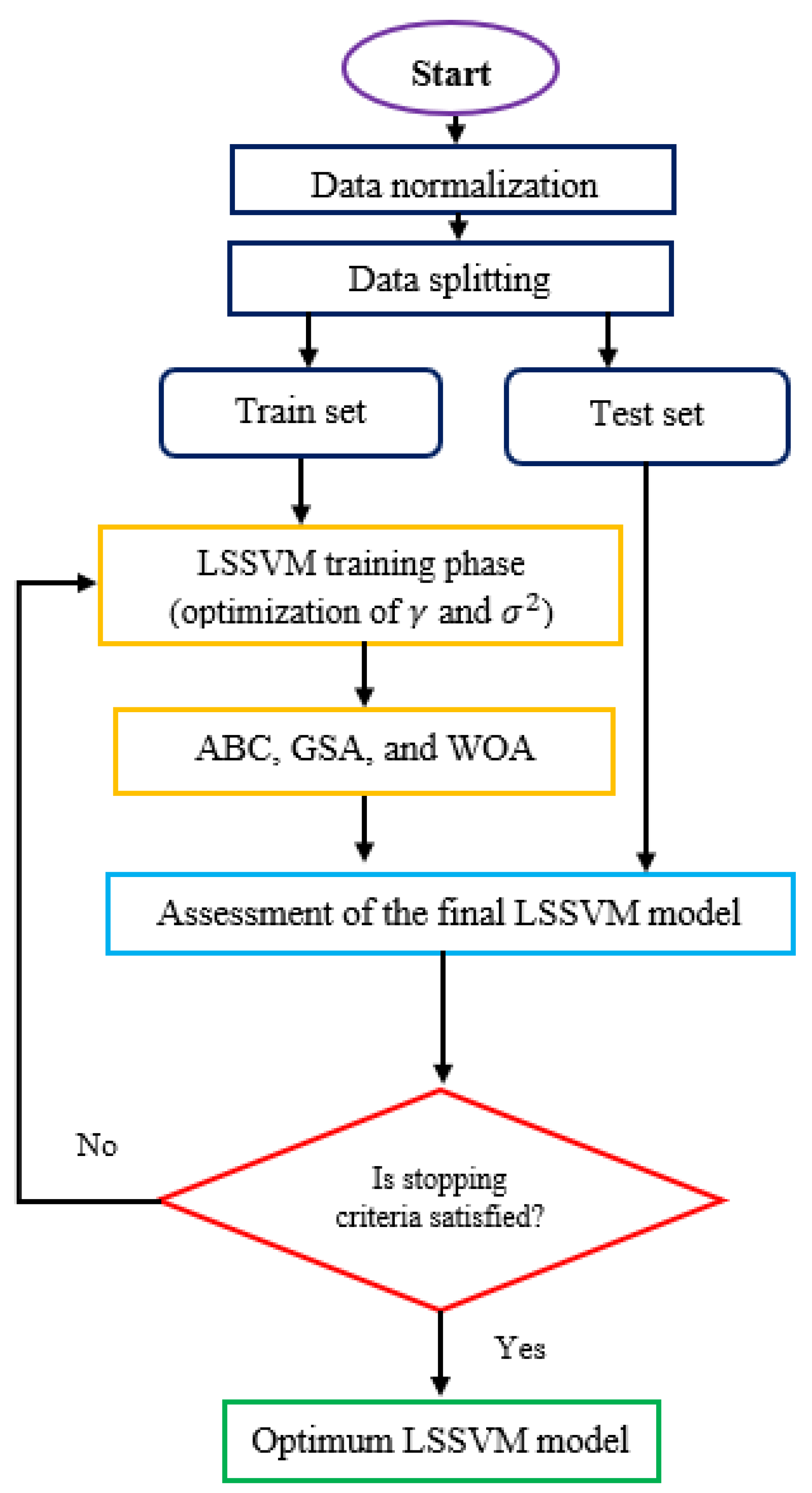
3.2.1. LSSVM Model
- (A)
- Gravitational search algorithm (GSA)
- (B)
- Whale optimization algorithm (WOA)
- (C)
- Artificial Bee Colony (ABC)
- -
- An initial population of bees is generated randomly. Each bee has its own position x. The numbers of employed and onlookers are the same in the population. A fitness function is considered for assessing the quality of the bees.
- -
- Employed bees: this step consists of updating the positions of bees at the generation () using the following equation:
- -
- Onlooker bees: by carrying out the previous step which emulates the exploitation phase, the gained information by the employed bees is exposed to the onlookers, which select the proper ones by applying the following equation bases on the probability :
- -
- Scout bees: this step consists of randomly changing the position of a given employed bee after a defined number of generations if it does not show any improvements in its fitness quality.
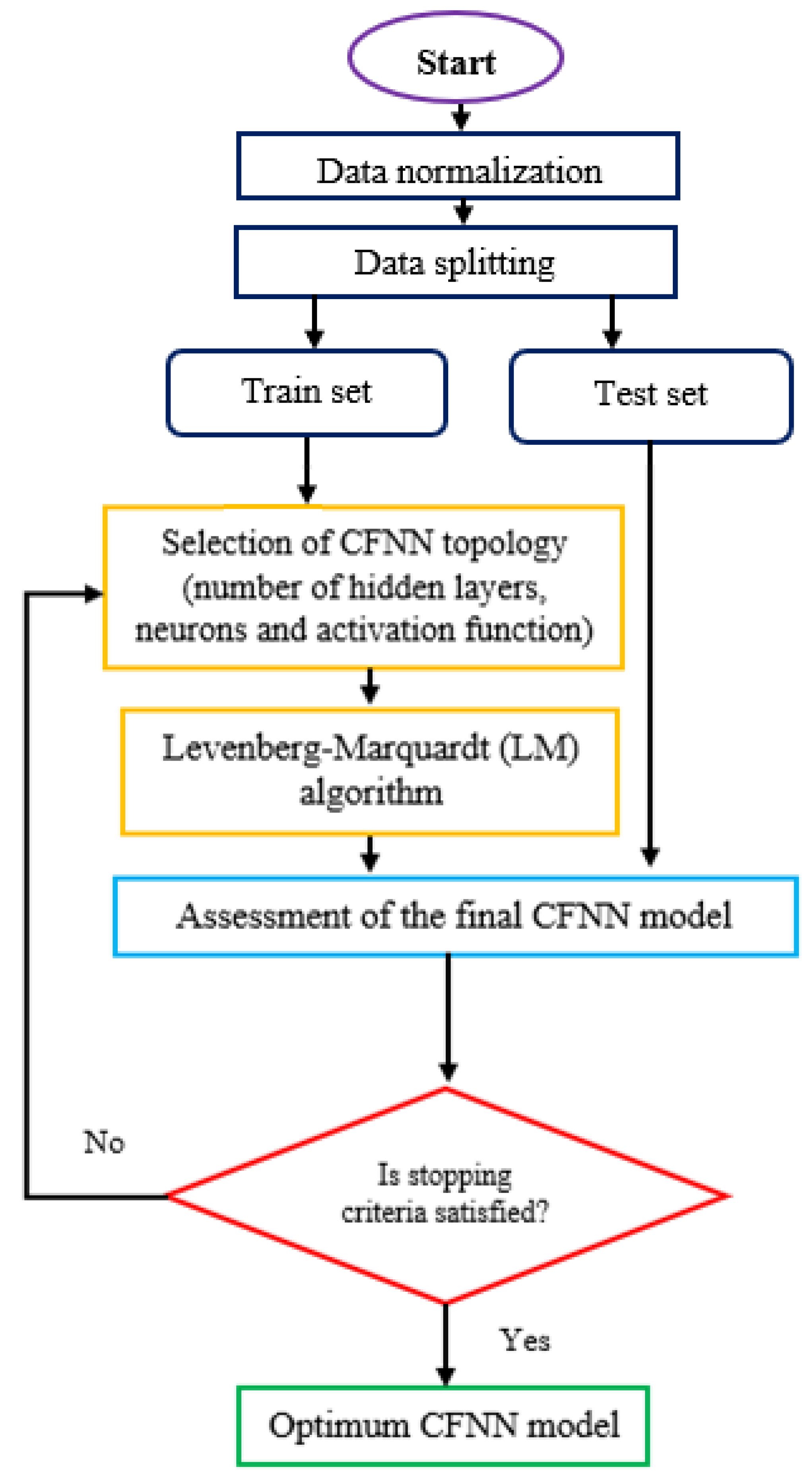
3.2.2. CFNN Model
3.2.3. Model Performance Evaluation
4. Development of Predictive Models
5. Results and Discussion
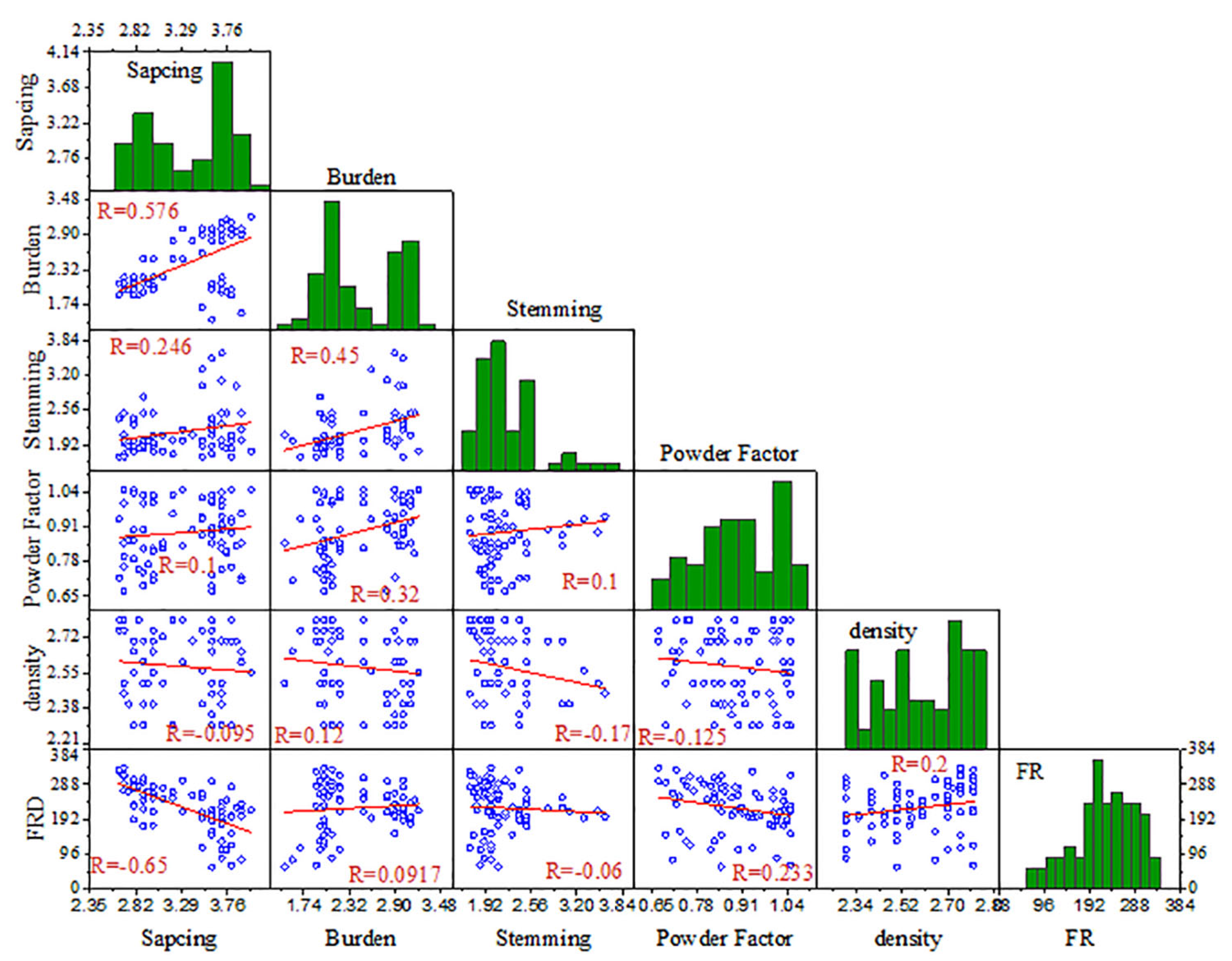
5.1. Exploratory Analysis
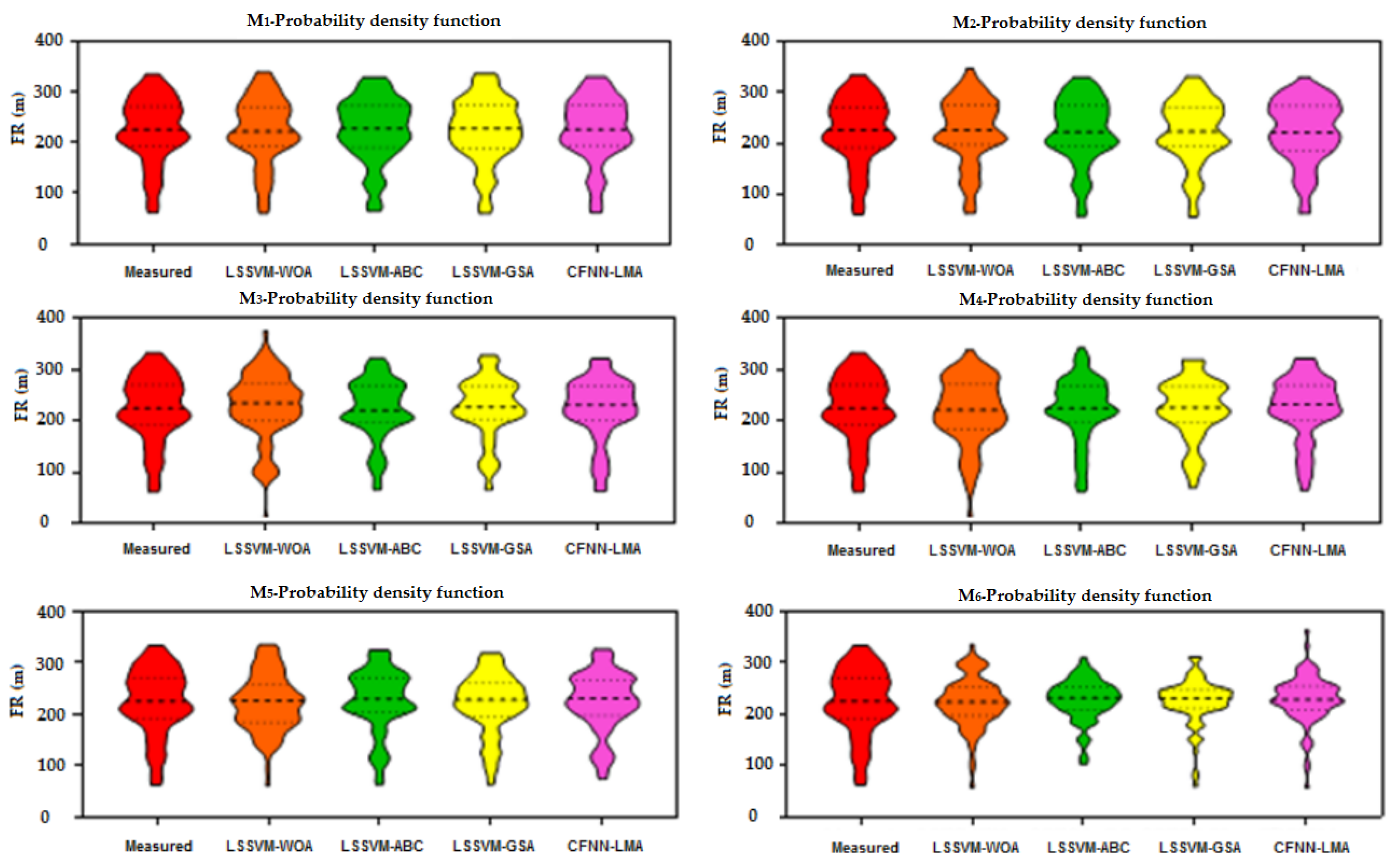
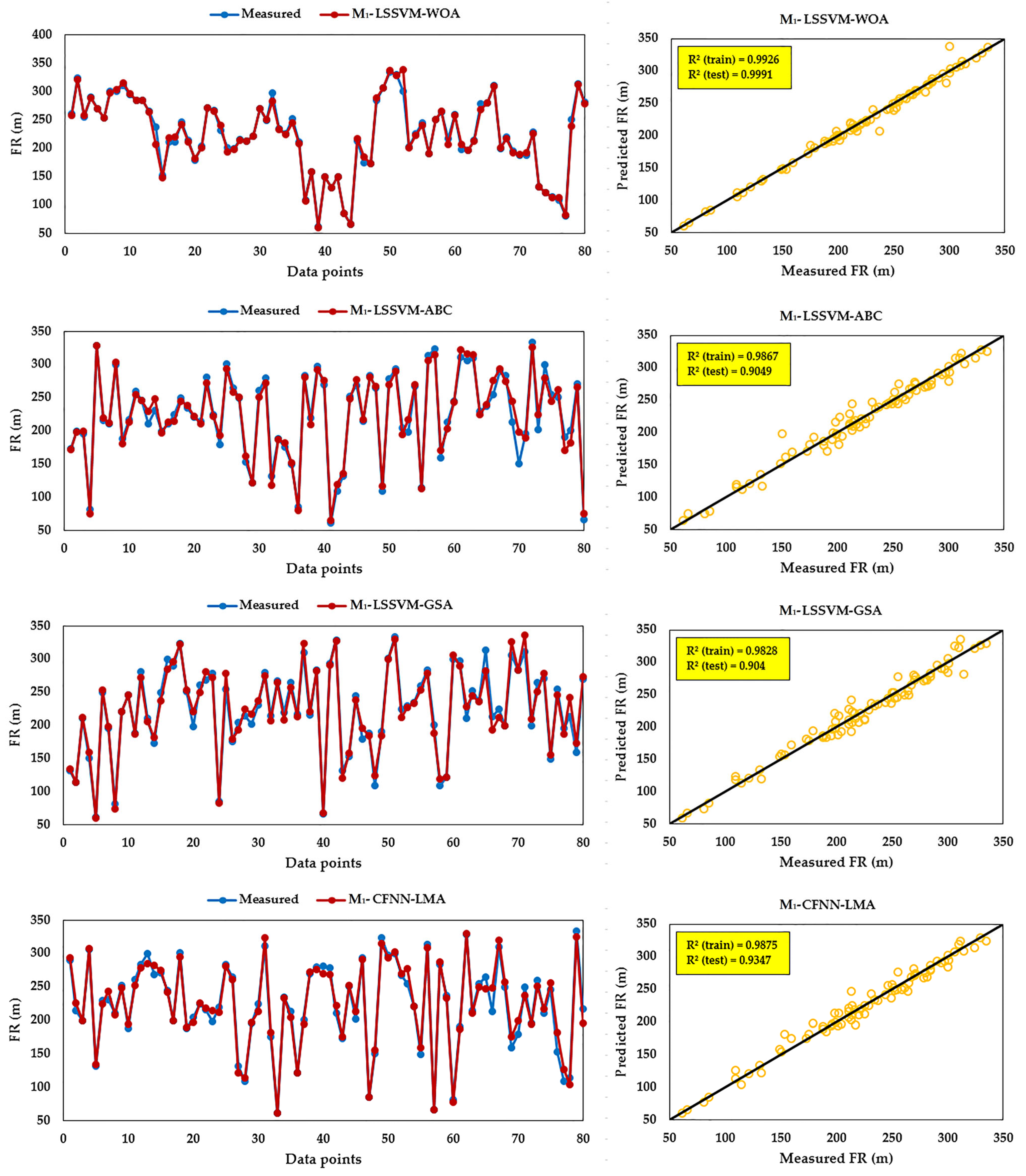
5.2. Modelling Results
6. Conclusions
Author Contributions
Funding
Institutional Review Board Statement
Informed Consent Statement
Data Availability Statement
Acknowledgments
Conflicts of Interest
References
- Raina, A.K.; Chakraborty, A.K.; Choudhury, P.B.; Sinha, A. Flyrock danger zone demarcation in opencast mines: A risk based approach. Bull. Eng. Geol. Environ. 2011, 70, 163–172. [Google Scholar] [CrossRef]
- Stojadinovic, S.; Pantovic, R.; Zikic, M. Prediction of flyrock trajectories for forensic applications using ballistic flight equations. Int. J. Rock Mech. Min. Sci. 2011, 48, 1086–1094. [Google Scholar] [CrossRef]
- Rad, H.N.; Hasanipanah, M.; Rezaei, M.; Eghlim, A.L. Developing a least squares support vector machine for estimating the blast-induced flyrock. Eng. Comput. 2018, 34, 709–717. [Google Scholar] [CrossRef]
- Jamei, M.; Hasanipanah, M.; Karbasi, M.; Ahmadianfar, I.; Taherifar, S. Prediction of flyrock induced by mine blasting using a novel kernel-based extreme learning machine. J. Rock Mech. Geotech. Eng. 2021, 13, 1438–1451. [Google Scholar] [CrossRef]
- Yari, M.; Armaghani, D.J.; Maraveas, C.; Ejlali, A.N.; Mohamad, E.T.; Asteris, P.G. Several Tree-Based Solutions for Predicting Flyrock Distance Due to Mine Blasting. Appl. Sci. 2023, 13, 1345. [Google Scholar] [CrossRef]
- Raina, A.K.; Chakraborty, A.K.; More, R.; Choudhury, P.B. Design of factor of safety based criterion for control of flyrock/throw and optimum fragmentation. J. Inst. Eng. Ser. A 2007, 87, 13–17. [Google Scholar]
- Ghasemi, E.; Sari, M.; Ataei, M. Development of an empirical model for predicting the effects of controllable blasting parameters on flyrock distance in surface mines. Int. J. Rock Mech. Min. Sci. 2012, 52, 163–170. [Google Scholar] [CrossRef]
- Armaghani, D.J.; Mahdiyar, A.; Hasanipanah, M.; Shirani Faradonbeh, R.; Khandelwal, M.; Bakhshandeh Amnieh, H. Risk assessment and prediction of flyrock distance by combined multiple regression analysis and monte-carlo simulation of quarry blasting. Rock Mech. Rock Eng. 2016, 49, 3631–3641. [Google Scholar] [CrossRef]
- Hasanipanah, M.; Jahed Armaghani, D.; Bakhshandeh Amnieh, H.; Abd Majid, M.Z.; Tahir, M. Application of PSO to develop a powerful equation for prediction of flyrock due to blasting. Neural Comput. Appl. 2017, 28, 1043–1050. [Google Scholar] [CrossRef]
- Hasanipanah, M.; Armaghani, D.J.; Amnieh, H.B.; Koopialipoor, M.; Arab, H. A risk based technique to analyze flyrock results through rock engineering system. Geotech. Geol. Eng. 2018, 36, 2247–2260. [Google Scholar] [CrossRef]
- Raina, A.K.; Murthy, V.; Soni, A.K. Flyrock in bench blasting: A comprehensive review. Bull. Eng. Geol. Environ. 2014, 73, 1199–1209. [Google Scholar] [CrossRef]
- Jahed Armaghani, D.; Hajihassani, M.; Monjezi, M.; Edy Tonnizam, M.; Marto, A.; Moghaddam, M.R. Application of two intelligent systems in predicting environmental impacts of quarry blasting. Arab. J. Geosci. 2015, 8, 9647–9665. [Google Scholar] [CrossRef]
- Little, T.N.; Blair, D.P. Mechanistic Monte Carlo models for analysis of flyrock risk. Rock Fragm. Blasting 2010, 9, 641–647. [Google Scholar]
- Kutter, H.K.; Fairhurst, C. On the fracture process in blasting. Int. J. Rock Mech. Min. Sci. Geomech. Abstr. 1971, 8, 181–202. [Google Scholar] [CrossRef]
- Liu, K.; Li, X.; Hao, H.; Li, X.; Sha, Y.; Wang, W.; Liu, X. Study on the raising technique using one blast based on the combination of long-hole presplitting and vertical crater retreat multiple-deck shots. Int. J. Rock Mech. Min. Sci. 2019, 113, 41–58. [Google Scholar] [CrossRef]
- Chao, Z.; Ma, G.; Wang, M. Experimental and numerical modelling of the mechanical behaviour of low-permeability sandstone considering hydromechanics. Mech. Mater. 2020, 148, 103454. [Google Scholar] [CrossRef]
- Wang, M.; Wang, F.; Zhu, Z.; Dong, Y.; Mousavi Nezhad, M.; Zhou, L. Modelling of crack propagation in rocks under SHPB impacts using a damage method. Fatigue Fract. Eng. Mater. Struct. 2019, 42, 1699–1710. [Google Scholar] [CrossRef]
- Wang, M.; Ma, G.; Wang, F. Numerically investigation on blast-induced wave propagation in catastrophic large-scale bedding rockslide. Landslides 2021, 18, 785–797. [Google Scholar] [CrossRef]
- Hajibagherpour, A.R.; Mansouri, H.; Bahaaddini, M. Numerical modeling of the fractured zones around a blasthole. Comput. Geotech. 2020, 123, 103535. [Google Scholar] [CrossRef]
- Trivedi, R.; Singh, T.N.; Raina, A.K. Prediction of blast-induced flyrock in Indian limestone mines using neural networks. J. Rock Mech. Geotech. Eng. 2014, 6, 447–454. [Google Scholar] [CrossRef]
- Yang, H.; Koopialipoor, M.; Armaghani, D.J.; Gordan, B.; Khorami, M.; Tahir, M.M. Intelligent design of retaining wall structures under dynamic conditions. Steel Compos. Struct. 2019, 31, 629–640. [Google Scholar]
- Yang, H.; Liu, X.; Song, K. A novel gradient boosting regression tree technique optimized by improved sparrow search algorithm for predicting TBM penetration rate. Arab. J. Geosci. 2022, 15, 461. [Google Scholar] [CrossRef]
- Yang, H.; Song, K.; Zhou, J. Automated Recognition Model of Geomechanical Information Based on Operational Data of Tunneling Boring Machines. Rock Mech. Rock Eng. 2020, 55, 1499–1516. [Google Scholar] [CrossRef]
- Yang, H.; Wang, Z.; Kanglei, S. A new hybrid grey wolf optimizer-feature weighted-multiple kernel-support vector regression technique to predict TBM performance. Eng. Comput. 2020, 38, 2469–2485. [Google Scholar] [CrossRef]
- Zhang, X.; He, B.; Sabri, M.M.S.; Al-Bahrani, M.; Ulrikh, D.V. Soil Liquefaction Prediction Based on Bayesian Optimization and Support Vector Machines. Sustainability 2022, 14, 11944. [Google Scholar] [CrossRef]
- Khan, N.M.; Cao, K.; Yuan, Q.; Bin Mohd Hashim, M.H.; Rehman, H.; Hussain, S.; Emad, M.Z.; Ullah, B.; Shah, K.S.; Khan, S. Application of Machine Learning and Multivariate Statistics to Predict Uniaxial Compressive Strength and Static Young’s Modulus Using Physical Properties under Different Thermal Conditions. Sustainability 2022, 14, 9901. [Google Scholar] [CrossRef]
- Shahani, N.M.; Zheng, X.; Guo, X.; Wei, X. Machine Learning-Based Intelligent Prediction of Elastic Modulus of Rocks at Thar Coalfield. Sustainability 2022, 14, 3689. [Google Scholar] [CrossRef]
- Yu, Q.; Monjezi, M.; Mohammed, A.S.; Dehghani, H.; Armaghani, D.J.; Ulrikh, D.V. Optimized Support Vector Machines Combined with Evolutionary Random Forest for Prediction of Back-Break Caused by Blasting Operation. Sustainability 2021, 13, 12797. [Google Scholar] [CrossRef]
- Hasanipanah, M.; Bakhshandeh Amnieh, H. A fuzzy rule based approach to address uncertainty in risk assessment and prediction of blast-induced flyrock in a quarry. Nat. Resour. Res. 2020, 29, 669–689. [Google Scholar] [CrossRef]
- Huat, C.Y.; Moosavi, S.M.H.; Mohammed, A.S.; Armaghani, D.J.; Ulrikh, D.V.; Monjezi, M.; Hin Lai, S. Factors Influencing Pile Friction Bearing Capacity: Proposing a Novel Procedure Based on Gradient Boosted Tree Technique. Sustainability 2021, 13, 11862. [Google Scholar] [CrossRef]
- Hosseini, S.; Pourmirzaee, R.; Armaghani, D.J.; Sabri Sabri, M.M. Prediction of ground vibration due to mine blasting in a surface lead–zinc mine using machine learning ensemble techniques. Sci. Rep. 2023, 13, 6591. [Google Scholar] [CrossRef] [PubMed]
- Monjezi, M.; Mehrdanesh, A.; Malek, A.; Khandelwal, M. Evaluation of effect of blast design parameters on flyrock using artificial neural networks. Neural Comput. Appl. 2013, 23, 349–356. [Google Scholar] [CrossRef]
- Ghasemi, E.; Amini, H.; Ataei, M.; Khalokakaei, R. Application of artificial intelligence techniques for predicting the flyrock distance caused by blasting operation. Arab. J. Geosci. 2014, 7, 193–202. [Google Scholar] [CrossRef]
- Trivedi, R.; Singh, T.N.; Gupta, N. Prediction of blast-induced flyrock in opencast mines using ANN and ANFIS. Geotech. Geol. Eng. 2015, 33, 875–891. [Google Scholar] [CrossRef]
- Faradonbeh, R.S.; Armaghani, D.J.; Monjezi, M. Development of a new model for predicting flyrock distance in quarry blasting: A genetic programming technique. Bull. Eng. Geol. Environ. 2016, 75, 993–1006. [Google Scholar] [CrossRef]
- Ye, J.; Koopialipoor, M.; Zhou, J.; Jahed Armaghani, D.; He, X. A Novel Combination of Tree-Based Modeling and Monte Carlo Simulation for Assessing Risk Levels of Flyrock Induced by Mine Blasting. Nat. Resour. Res. 2021, 30, 225–243. [Google Scholar] [CrossRef]
- Hemmati Sarapardeh, A.; Larestani, A.; Nait Amar, M.; Hajirezaie, S. Applications of Artificial Intelligence Techniques in the Petroleum Industry; Gulf Professional Publishing: Houston, TX, USA, 2020. [Google Scholar] [CrossRef]
- Cai, M.; Hocine, O.; Salih Mohammed, A.; Chen, X.; Nait Amar, M.; Hasanipanah, M. Integrating the LSSVM and RBFNN models with three optimization algorithms to predict the soil liquefaction potential. Eng. Comput. 2021, 38, 3611–3623. [Google Scholar] [CrossRef]
- Suykens, J.A.K.; Vandewalle, J. Least squares support vector machine classifiers. Neural Process. Lett. 1999, 9, 293–300. [Google Scholar] [CrossRef]
- Forrester, A.I.J.; Sóbester, A.; Keane, A.J. Engineering Design via Surrogate Modelling: A Practical Guide; John Wiley & Sons: Hoboken, NJ, USA, 2008. [Google Scholar]
- Rashedi, E.; Nezamabadi-Pour, H.; Saryazdi, S. GSA: A gravitational search algorithm. Inf. Sci. 2009, 179, 2232–2248. [Google Scholar] [CrossRef]
- Mirjalili, S.; Lewis, A. The Whale Optimization Algorithm. Adv. Eng. Softw. 2016, 95, 51–67. [Google Scholar] [CrossRef]
- Karaboga, D. An Idea Based on Honey Bee Swarm for Numerical Optimization; Technical Report-TR06; Erciyes University, Engineering Faculty, Computer Engineering Department: Kayseri, Turkey, 2005. [Google Scholar]
- Karaboga, D.; Basturk, B. A powerful and efficient algorithm for numerical function optimization: Artificial bee colony (ABC) algorithm. J. Glob. Optim. 2007, 39, 459–471. [Google Scholar] [CrossRef]
- Nait Amar, M. Modelling solubility of sulfur in pure hydrogen sulfide and sour gas mixtures using rigorous machine learning methods. Int. J. Hydrogen Energy 2020, 45, 33274–33287. [Google Scholar] [CrossRef]
- Abujazar, M.S.S.; Fatihah, S.; Ibrahim, I.A.; Kabeel, A.E.; Sharil, S. Productivity modelling of a developed inclined stepped solar still system based on actual performance and using a cascaded forward neural network model. J. Clean. Prod. 2018, 170, 147–159. [Google Scholar] [CrossRef]
- Hemmati-Sarapardeh, A.; Varamesh, A.; Husein, M.M.; Karan, K. On the evaluation of the viscosity of nanofluid systems: Modeling and data assessment. Renew. Sustain. Energy Rev. 2018, 81, 313–329. [Google Scholar] [CrossRef]
- Hemmati-Sarapardeh, A.; Nait Amar, M.; Soltanian, M.R.; Dai, Z.; Zhang, X. Modeling CO2 Solubility in Water at High Pressure and Temperature Conditions. Energy Fuels 2020, 34, 4761–4776. [Google Scholar] [CrossRef]
- Huang, J.; Zhang, J.; Li, X.; Qiao, Y.; Zhang, R.; Kumar, G.S. Investigating the effects of ensemble and weight optimization approaches on neural networks’ performance to estimate the dynamic modulus of asphalt concrete. Road Mater. Pavement Des. 2022, 1–21. [Google Scholar] [CrossRef]
- Huang, J.; Zhou, M.; Zhang, J.; Ren, J.; Vatin, N.; Sabri, M. Development of a new stacking model to evaluate the strength parameters of concrete samples in laboratory. Iran. J. Sci. Technol. Trans. Civ. Eng. 2022, 46, 4355–4370. [Google Scholar] [CrossRef]
- Huang, J.; Zhou, M.; Zhang, J.; Ren, J.; Vatin, N.I.; Sabri, M.M.S. The use of GA and PSO in evaluating the shear strength of steel fiber reinforced concrete beams. KSCE J. Civ. Eng. 2022, 26, 3918–3931. [Google Scholar] [CrossRef]
- Huang, J.; Xue, J. Optimization of SVR functions for flyrock evaluation in mine blasting operations. Environ. Earth Sci. 2022, 81, 434. [Google Scholar] [CrossRef]
- Talebkeikhah, M.; Amar, M.N.; Naseri, A.; Humand, M.; Hemmati-Sarapardeh, A.; Dabir, B.; Seghier, M.E.A.B. Experimental measurement and compositional modeling of crude oil viscosity at reservoir conditions. J. Taiwan Inst. Chem. Eng. 2020, 109, 35–50. [Google Scholar] [CrossRef]
- Rostami, A.; Baghban, A.; Shirazian, S. On the evaluation of density of ionic liquids: Towards a comparative study. Chem. Eng. Res. Des. 2019, 147, 648–663. [Google Scholar] [CrossRef]
- Koopialipoor, M.; Fallah, A.; Armaghani, D.J.; Azizi, A.; Mohamad, E.T. Three hybrid intelligent models in estimating flyrock distance resulting from blasting. Eng. Comput. 2019, 35, 243–256. [Google Scholar] [CrossRef]
- Faradonbeh, R.S.; Armaghani, D.J.; Amnieh, H.B.; Mohamad, E.T. Prediction and minimization of blast-induced flyrock using gene expression programming and firefly algorithm. Neural Comput. Appl. 2018, 29, 269–281. [Google Scholar] [CrossRef]
- Zhou, J.; Aghili, N.; Ghaleini, E.N.; Bui, D.T.; Tahir, M.M.; Koopialipoor, M. A Monte Carlo simulation approach for effective assessment of flyrock based on intelligent system of neural network. Eng. Comput. 2019, 36, 713–723. [Google Scholar] [CrossRef]
- Nguyen, H.; Bui, X.-N.; Nguyen-Thoi, T.; Ragam, P.; Moayedi, H. Toward a state-of-the-art of fly-rock prediction technology in open-pit mines using EANNs model. Appl. Sci. 2019, 9, 4554. [Google Scholar] [CrossRef]
- Marto, A.; Hajihassani, M.; Jahed Armaghani, D.; Tonnizam Mohamad, E.; Makhtar, A.M. A novel approach for blast-induced flyrock prediction based on imperialist competitive algorithm and artificial neural network. Sci. World J. 2014, 2014, 643715. [Google Scholar] [CrossRef]


| Algorithm | Parameter | Value |
|---|---|---|
| ABC | Number of employer bees | 20 |
| Number of onlooker bees | 20 | |
| Number of generations | 30 | |
| Number of generations to scout bees | 4 | |
| GSA | and | [0, 1] |
| Number of generations | 30 | |
| Number of individuals | 40 | |
| WOA | a | 2 to 0 |
| r | [0, 1] | |
| Number of generations | 30 | |
| Number of whales | 40 |
| Metric/Feature | S (m) | B (m) | ST (m) | PF (kg/m3) | Density (gr/cm3) | FR (m) |
|---|---|---|---|---|---|---|
| Minimum | 2.65 | 1.5 | 1.7 | 0.67 | 2.3 | 61 |
| Maximum | 4 | 3.2 | 3.6 | 1.05 | 2.8 | 334 |
| Mean | 3.324 | 2.415 | 2.171 | 0.8908 | 2.579 | 223.5 |
| Std. Deviation | 0.4228 | 0.4776 | 0.4022 | 0.113 | 0.1684 | 64.61 |
| CV | 12.72% | 19.78% | 18.53% | 12.69% | 6.529% | 28.91% |
| Skewness | −0.2032 | 0.2017 | 1.608 | −0.2148 | −0.2942 | −0.5848 |
| Kurtosis | −1.556 | −1.518 | 2.82 | −1.058 | −1.247 | −0.1065 |
| Scheme | Model | Statistical Criteria | Train Data | Test Data | All Data |
|---|---|---|---|---|---|
| M1 | CFNN-LMA | R2 | 0.9875 | 0.9347 | 0.977 |
| AARE | 2.5163 | 7.512 | 3.5154 | ||
| RMSE | 7.2292 | 16.5215 | 9.8184 | ||
| LSSVM-ABC | R2 | 0.9867 | 0.9049 | 0.971 | |
| AARE | 3.0419 | 8.0032 | 4.0341 | ||
| RMSE | 7.4089 | 19.439 | 10.9311 | ||
| LSSVM-GSA | R2 | 0.9828 | 0.904 | 0.967 | |
| AARE | 3.4215 | 5.5193 | 3.8411 | ||
| RMSE | 8.7308 | 16.1775 | 10.6453 | ||
| LSSVM-WOA | R2 | 0.9926 | 0.9991 | 0.9943 | |
| AARE | 1.6473 | 1.3017 | 1.5782 | ||
| RMSE | 7.4847 | 3.4209 | 6.8671 | ||
| M2 | CFNN-LMA | R2 | 0.9812 | 0.9366 | 0.972 |
| AARE | 2.9261 | 8.5748 | 4.0558 | ||
| RMSE | 8.4645 | 20.2612 | 11.8077 | ||
| LSSVM-ABC | R2 | 0.9769 | 0.9235 | 0.9675 | |
| AARE | 3.7643 | 7.083 | 4.428 | ||
| RMSE | 9.8655 | 16.7483 | 11.5743 | ||
| LSSVM-GSA | R2 | 0.9754 | 0.9054 | 0.9614 | |
| AARE | 4.254 | 6.5356 | 4.7103 | ||
| RMSE | 10.3962 | 18.0443 | 12.312 | ||
| LSSVM-WOA | R2 | 0.9871 | 0.9896 | 0.9875 | |
| AARE | 2.6662 | 2.8723 | 2.7074 | ||
| RMSE | 10.105 | 10.4268 | 10.1702 | ||
| M3 | CFNN-LMA | R2 | 0.883 | 0.9172 | 0.89 |
| AARE | 7.2573 | 8.2441 | 7.4546 | ||
| RMSE | 21.9097 | 18.6501 | 21.2977 | ||
| LSSVM-ABC | R2 | 0.9191 | 0.7622 | 0.8811 | |
| AARE | 6.7642 | 12.4379 | 7.8989 | ||
| RMSE | 17.7366 | 34.5376 | 22.1413 | ||
| LSSVM-GSA | R2 | 0.8874 | 0.7979 | 0.8714 | |
| AARE | 7.8757 | 13.615 | 9.0236 | ||
| RMSE | 21.7035 | 27.6908 | 23.0259 | ||
| LSSVM-WOA | R2 | 0.9625 | 0.9398 | 0.9305 | |
| AARE | 6.6657 | 21.8618 | 9.7049 | ||
| RMSE | 17.5076 | 43.8141 | 25.0828 | ||
| M4 | CFNN-LMA | R2 | 0.8878 | 0.8706 | 0.8856 |
| AARE | 6.9643 | 10.5219 | 7.6758 | ||
| RMSE | 21.6209 | 22.0891 | 21.7153 | ||
| LSSVM-ABC | R2 | 0.892 | 0.8572 | 0.8849 | |
| AARE | 7.0333 | 9.8644 | 7.5995 | ||
| RMSE | 20.9307 | 24.9094 | 21.7846 | ||
| LSSVM-GSA | R2 | 0.8689 | 0.8748 | 0.8707 | |
| AARE | 8.1285 | 11.6169 | 8.8262 | ||
| RMSE | 22.7463 | 24.3938 | 23.0852 | ||
| LSSVM-WOA | R2 | 0.9921 | 0.9201 | 0.9777 | |
| AARE | 2.7384 | 14.8704 | 5.1648 | ||
| RMSE | 8.0666 | 31.6042 | 15.8689 | ||
| M5 | CFNN-LMA | R2 | 0.8879 | 0.8456 | 0.8791 |
| AARE | 7.6983 | 11.2721 | 8.413 | ||
| RMSE | 21.3743 | 25.7841 | 22.326 | ||
| LSSVM-ABC | R2 | 0.8891 | 0.8376 | 0.8823 | |
| AARE | 8.3536 | 7.5541 | 8.1937 | ||
| RMSE | 22.1859 | 21.3895 | 22.0289 | ||
| LSSVM-GSA | R2 | 0.8983 | 0.831 | 0.8825 | |
| AARE | 6.6676 | 11.6499 | 7.6641 | ||
| RMSE | 19.9291 | 28.846 | 22.0035 | ||
| LSSVM-WOA | R2 | 0.8979 | 0.7985 | 0.8859 | |
| AARE | 12.374 | 13.7799 | 12.6551 | ||
| RMSE | 29.5911 | 30.7061 | 29.8175 | ||
| M6 | CFNN-LMA | R2 | 0.4324 | 0.3195 | 0.4186 |
| AARE | 17.817 | 30.9799 | 20.4496 | ||
| RMSE | 46.3091 | 58.3475 | 48.9542 | ||
| LSSVM-ABC | R2 | 0.4856 | 0.1575 | 0.4327 | |
| AARE | 17.9507 | 30.1723 | 20.395 | ||
| RMSE | 44.6322 | 61.0195 | 48.356 | ||
| LSSVM-GSA | R2 | 0.5574 | 0.4669 | 0.4329 | |
| AARE | 18.587 | 24.6491 | 19.7994 | ||
| RMSE | 44.7295 | 60.6898 | 48.3449 | ||
| LSSVM-WOA | R2 | 0.806 | 0.3616 | 0.7228 | |
| AARE | 15.5962 | 22.1002 | 16.897 | ||
| RMSE | 40.172 | 58.5744 | 44.466 |
| Overall R2 | Overall RMSE | |
|---|---|---|
| Fold 1 | 0.9759 | 9.8664 |
| Fold 2 | 0.9761 | 9.8601 |
| Fold 3 | 0.9754 | 9.9361 |
| Fold 4 | 0.9762 | 9.8597 |
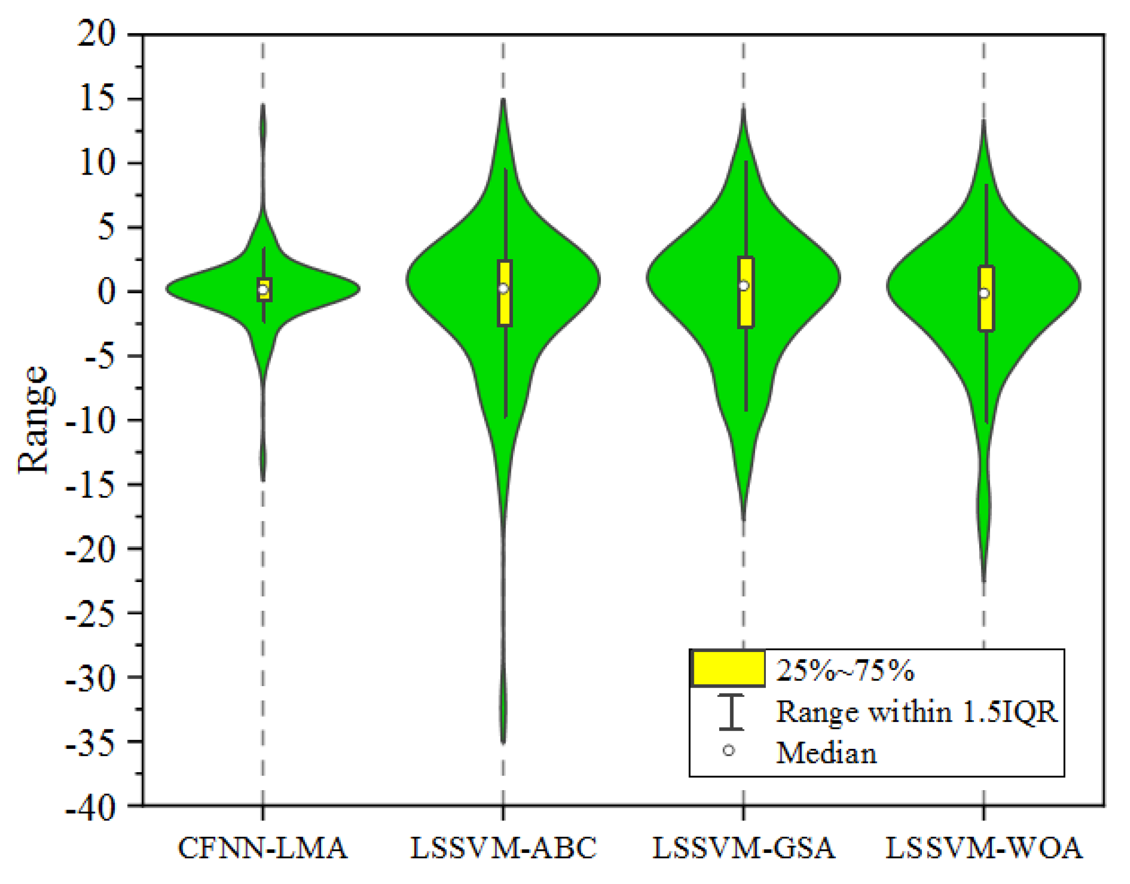
| Model | CFNN-LMA | LSSVM-ABC | LSSVM-GSA | LSSVM-WOA |
|---|---|---|---|---|
| Q25%-RD% | −0.5566 | −2.778 | −2.712 | −2.976 |
| Q75%-RD% | 1.093 | 2.504 | 2.716 | 2.105 |
| IQR-RD% | 1.650 | 5.282 | 5.428 | 5.081 |
Disclaimer/Publisher’s Note: The statements, opinions and data contained in all publications are solely those of the individual author(s) and contributor(s) and not of MDPI and/or the editor(s). MDPI and/or the editor(s) disclaim responsibility for any injury to people or property resulting from any ideas, methods, instructions or products referred to in the content. |
© 2023 by the authors. Licensee MDPI, Basel, Switzerland. This article is an open access article distributed under the terms and conditions of the Creative Commons Attribution (CC BY) license (https://creativecommons.org/licenses/by/4.0/).
Share and Cite
Ding, X.; Jamei, M.; Hasanipanah, M.; Abdullah, R.A.; Le, B.N. Optimized Data-Driven Models for Prediction of Flyrock due to Blasting in Surface Mines. Sustainability 2023, 15, 8424. https://doi.org/10.3390/su15108424
Ding X, Jamei M, Hasanipanah M, Abdullah RA, Le BN. Optimized Data-Driven Models for Prediction of Flyrock due to Blasting in Surface Mines. Sustainability. 2023; 15(10):8424. https://doi.org/10.3390/su15108424
Chicago/Turabian StyleDing, Xiaohua, Mehdi Jamei, Mahdi Hasanipanah, Rini Asnida Abdullah, and Binh Nguyen Le. 2023. "Optimized Data-Driven Models for Prediction of Flyrock due to Blasting in Surface Mines" Sustainability 15, no. 10: 8424. https://doi.org/10.3390/su15108424