

Investigating the Effect of Parameters on Confinement Coefficient of Reinforced Concrete Using Development of Learning Machine Models
 ,
,  and
and
Abstract
:1. Introduction
2. Experimental Setting
2.1. Data
2.2. Previous Analytical Models
3. Methodology
3.1. Inspiration
3.2. Developing SDO
4. Simulation Procedure
4.1. Pre-Training
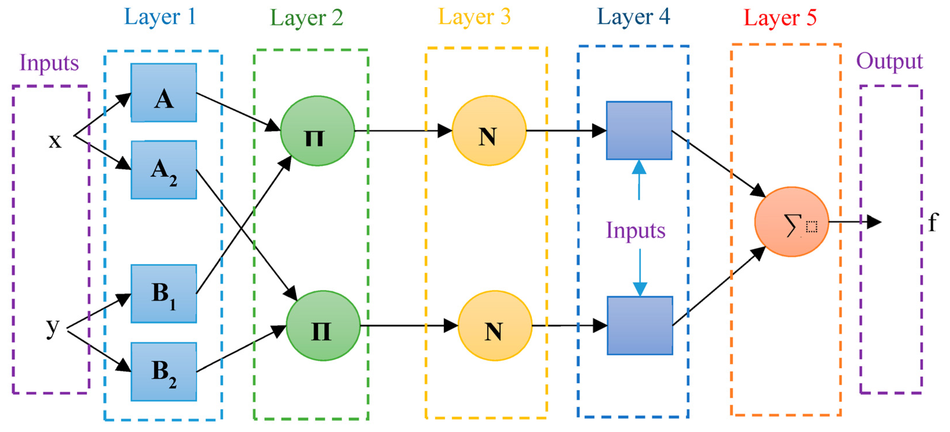
4.2. ANFIS
4.3. SDO-ANFIS
5. Results and Discussion
6. Conclusions
- -
- Among the 14 different combinations, the data that included six inputs had less errors;
- -
- Using the model developed in this research and according to the six input parameters, an exact estimation of Ks can be obtained. The experimental data are the main source for the hybrid model training. The quality and quantity of these data thus directly affect the hybrid model performance. In fact, the hybrid model error reduces as the volume of data increases;
- -
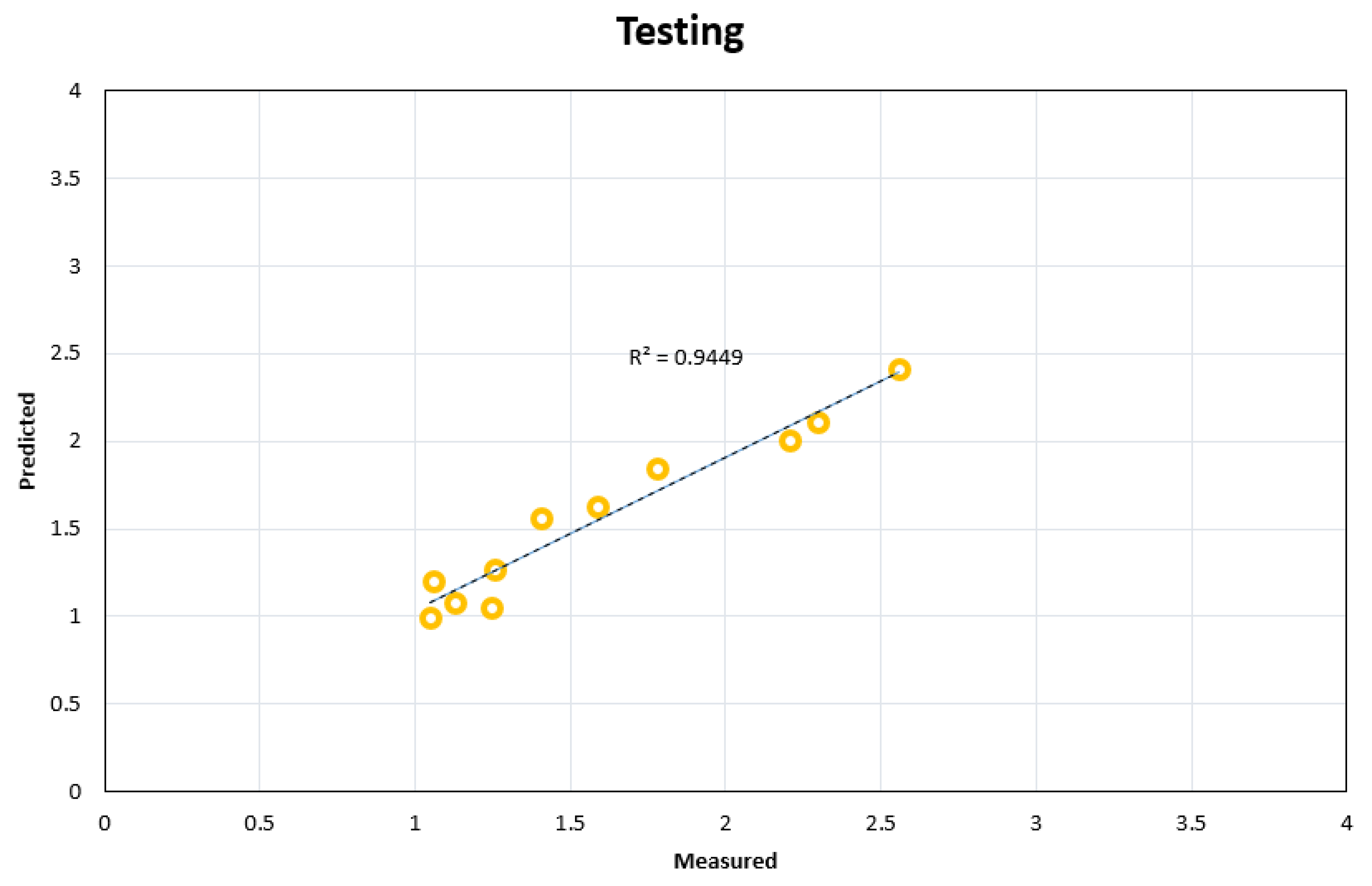
- The results of the ANFIS base model for the training and testing sections were R2 = 0.8961 and 0.8821, respectively, and with the development of the model with the SDO algorithm, their accuracy increased to 0.9501 and 0.9449, respectively;
- -
- The results show that the RMSE of hybrid models provide more appropriate values in predicting the Ks in comparison with the basic ANFIS. For the test results, the new SDO-ANFIS model obtained values of RMSE = 0.134, which performed better than other models. Therefore, the SDO-ANFIS model has higher accuracy and less error than other hybrid models for Ks prediction.
Author Contributions
Funding
Institutional Review Board Statement
Informed Consent Statement
Data Availability Statement
Acknowledgments
Conflicts of Interest
References
- Vincevica-Gaile, Z.; Teppand, T.; Kriipsalu, M.; Krievans, M.; Jani, Y.; Klavins, M.; Hendroko Setyobudi, R.; Grinfelde, I.; Rudovica, V.; Tamm, T. Towards sustainable soil stabilization in peatlands: Secondary raw materials as an alternative. Sustainability 2021, 13, 6726. [Google Scholar] [CrossRef]
- Kent, D.C.; Park, R. Flexural members with confined concrete. J. Struct. Div. 1971, 97, 1969–1990. [Google Scholar] [CrossRef]
- Park, R.; Priestley, M.J.; Gill, W.D. Ductility of square-confined concrete columns. J. Struct. Div. 1982, 108, 929–950. [Google Scholar] [CrossRef]
- Sheikh, S.A.; Uzumeri, S.M. Analytical model for concrete confinement in tied columns. J. Struct. Div. 1982, 108, 2703–2722. [Google Scholar] [CrossRef]
- Sheikh, S.A.; Uzumeri, S.M. Strength and ductility of tied concrete columns. J. Struct. Div. 1980, 106, 1079–1102. [Google Scholar] [CrossRef]
- Saatcioglu, M.; Razvi, S.R. Strength and ductility of confined concrete. J. Struct. Eng. 1992, 118, 1590–1607. [Google Scholar] [CrossRef]
- Razvi, S.; Saatcioglu, M. Confinement model for high-strength concrete. J. Struct. Eng. 1999, 125, 281–289. [Google Scholar] [CrossRef]
- Chung, H.-S.; Yang, K.-H.; Lee, Y.-H.; Eun, H.-C. Stress–strain curve of laterally confined concrete. Eng. Struct. 2002, 24, 1153–1163. [Google Scholar] [CrossRef]
- Flood, I. A neural network approach to the sequencing of construction tasks. In Proceedings of the Proceedings of the Sixth International Symposium on Automation and Robotics in Construction, Construction Industry Institute, San Francisco, CA, USA, 6–8 June 1989. [Google Scholar]
- Ren, L.; Zhao, Z. An optimal neural network and concrete strength modeling. Adv. Eng. Softw. 2002, 33, 117–130. [Google Scholar] [CrossRef]
- Cladera, A.; Marí, A.R. Shear design procedure for reinforced normal and high-strength concrete beams using artificial neural networks. Part I: Beams without stirrups. Eng. Struct. 2004, 26, 917–926. [Google Scholar] [CrossRef]
- Naeej, M.; Bali, M.; Naeej, M.R.; Amiri, J.V. Prediction of lateral confinement coefficient in reinforced concrete columns using M5′ machine learning method. KSCE J. Civ. Eng. 2013, 17, 1714–1719. [Google Scholar] [CrossRef]
- Yetilmezsoy, K.; Sihag, P.; Kıyan, E.; Doran, B. A benchmark comparison and optimization of Gaussian process regression, support vector machines, and M5P tree model in approximation of the lateral confinement coefficient for CFRP-wrapped rectangular/square RC columns. Eng. Struct. 2021, 246, 113106. [Google Scholar] [CrossRef]
- Alacalı, S.N.; Akbaş, B.; Doran, B. Prediction of lateral confinement coefficient in reinforced concrete columns using neural network simulation. Appl. Soft Comput. 2011, 11, 2645–2655. [Google Scholar] [CrossRef]
- Koopialipoor, M.; Fahimifar, A.; Ghaleini, E.N.; Momenzadeh, M.; Armaghani, D.J. Development of a new hybrid ANN for solving a geotechnical problem related to tunnel boring machine performance. Eng. Comput. 2020, 36, 345–357. [Google Scholar] [CrossRef]
- Koopialipoor, M.; Ghaleini, E.N.; Tootoonchi, H.; Jahed Armaghani, D.; Haghighi, M.; Hedayat, A. Developing a new intelligent technique to predict overbreak in tunnels using an artificial bee colony-based ANN. Environ. Earth Sci. 2019, 78, 165. [Google Scholar] [CrossRef]
- Zhou, J.; Guo, H.; Koopialipoor, M.; Armaghani, D.J.; Tahir, M.M. Investigating the effective parameters on the risk levels of rockburst phenomena by developing a hybrid heuristic algorithm. Eng. Comput. 2021, 37, 1679–1694. [Google Scholar] [CrossRef]
- Yang, H.; Koopialipoor, M.; Armaghani, D.J.; Gordan, B.; Khorami, M.; Tahir, M.M. Intelligent design of retaining wall structures under dynamic conditions. STEEL Compos. Struct. 2019, 31, 629–640. [Google Scholar]
- Mohamad, E.T.; Koopialipoor, M.; Murlidhar, B.R.; Rashiddel, A.; Hedayat, A.; Armaghani, D.J. A new hybrid method for predicting ripping production in different weathering zones through in-situ tests. Measurement 2019, 147, 106826. [Google Scholar] [CrossRef]
- Sharbati, R.; Khoshnoudian, F.; Koopialipoor, M.; Tahir, M.M. Applying dual-tree complex discrete wavelet transform and gamma modulating function for simulation of ground motions. Eng. Comput. 2021, 37, 1519–1535. [Google Scholar] [CrossRef]
- Zhou, J.; Li, C.; Koopialipoor, M.; Jahed Armaghani, D.; Thai Pham, B. Development of a new methodology for estimating the amount of PPV in surface mines based on prediction and probabilistic models (GEP-MC). Int. J. Min. Reclam. Environ. 2021, 35, 48–68. [Google Scholar] [CrossRef]
- Mahdiyar, A.; Jahed Armaghani, D.; Koopialipoor, M.; Hedayat, A.; Abdullah, A.; Yahya, K. Practical Risk Assessment of Ground Vibrations Resulting from Blasting, Using Gene Expression Programming and Monte Carlo Simulation Techniques. Appl. Sci. 2020, 10, 472. [Google Scholar] [CrossRef]
- Koopialipoor, M.; Tootoonchi, H.; Jahed Armaghani, D.; Tonnizam Mohamad, E.; Hedayat, A. Application of deep neural networks in predicting the penetration rate of tunnel boring machines. Bull. Eng. Geol. Environ. 2019, 78, 6347–6360. [Google Scholar] [CrossRef]
- Tang, D.; Gordan, B.; Koopialipoor, M.; Jahed Armaghani, D.; Tarinejad, R.; Thai Pham, B.; Huynh, V. Van Seepage Analysis in Short Embankments Using Developing a Metaheuristic Method Based on Governing Equations. Appl. Sci. 2020, 10, 1761. [Google Scholar] [CrossRef] [Green Version]
- Xu, C.; Gordan, B.; Koopialipoor, M.; Armaghani, D.J.; Tahir, M.M.; Zhang, X. Improving Performance of Retaining Walls Under Dynamic Conditions Developing an Optimized ANN Based on Ant Colony Optimization Technique. IEEE Access 2019, 7, 94692–94700. [Google Scholar] [CrossRef]
- Asteris, P.G.; Plevris, V. Anisotropic masonry failure criterion using artificial neural networks. Neural Comput. Appl. 2017, 28, 2207–2229. [Google Scholar] [CrossRef]
- Zhang, H.; Nguyen, H.; Bui, X.-N.; Pradhan, B.; Asteris, P.G.; Costache, R.; Aryal, J. A generalized artificial intelligence model for estimating the friction angle of clays in evaluating slope stability using a deep neural network and Harris Hawks optimization algorithm. Eng. Comput. 2022, 38, 3901–3914. [Google Scholar] [CrossRef]
- Bokolo, A.J. Green campus paradigms for sustainability attainment in higher education institutions—A comparative study. J. Sci. Technol. Policy Manag. 2020, 12, 117–148. [Google Scholar]
- Shirkhani, A.; Davarnia, D.; Azar, B.F. Prediction of bond strength between concrete and rebar under corrosion using ANN. Comput. Concr. 2019, 23, 273–279. [Google Scholar]
- Liu, Z.; Armaghani, D.J.; Fakharian, P.; Li, D.; Ulrikh, D.V.; Orekhova, N.N.; Khedher, K.M. Rock Strength Estimation Using Several Tree-Based ML Techniques. C. Model. Eng. Sci. 2022, 133, 799–824. [Google Scholar] [CrossRef]
- Asteris, P.G.; Rizal, F.I.M.; Koopialipoor, M.; Roussis, P.C.; Ferentinou, M.; Armaghani, D.J.; Gordan, B. Slope Stability Classification under Seismic Conditions Using Several Tree-Based Intelligent Techniques. Appl. Sci. 2022, 12, 1753. [Google Scholar] [CrossRef]
- Asteris, P.G.; Lourenço, P.B.; Roussis, P.C.; Adami, C.E.; Armaghani, D.J.; Cavaleri, L.; Chalioris, C.E.; Hajihassani, M.; Lemonis, M.E.; Mohammed, A.S. Revealing the nature of metakaolin-based concrete materials using artificial intelligence techniques. Constr. Build. Mater. 2022, 322, 126500. [Google Scholar] [CrossRef]
- Armaghani, D.J.; Harandizadeh, H.; Momeni, E.; Maizir, H.; Zhou, J. An Optimized System of GMDH-ANFIS Predictive Model by ICA for Estimating Pile Bearing Capacity; Springer: Dodrecht, The Netherlands, 2022; Volume 55, ISBN 0123456789. [Google Scholar]
- Shan, F.; He, X.; Armaghani, D.J.; Zhang, P.; Sheng, D. Success and challenges in predicting TBM penetration rate using recurrent neural networks. Tunn. Undergr. Sp. Technol. 2022, 130, 104728. [Google Scholar] [CrossRef]
- Mahmood, W.; Mohammed, A.S.; Asteris, P.G.; Kurda, R.; Armaghani, D.J. Modeling Flexural and Compressive Strengths Behaviour of Cement-Grouted Sands Modified with Water Reducer Polymer. Appl. Sci. 2022, 12, 1016. [Google Scholar] [CrossRef]
- Hasanipanah, M.; Monjezi, M.; Shahnazar, A.; Armaghani, D.J.; Farazmand, A. Feasibility of indirect determination of blast induced ground vibration based on support vector machine. Measurement 2015, 75, 289–297. [Google Scholar] [CrossRef]
- Chen, L.; Asteris, P.G.; Tsoukalas, M.Z.; Armaghani, D.J.; Ulrikh, D.V.; Yari, M. Forecast of Airblast Vibrations Induced by Blasting Using Support Vector Regression Optimized by the Grasshopper Optimization (SVR-GO) Technique. Appl. Sci. 2022, 12, 9805. [Google Scholar] [CrossRef]
- Barkhordari, M.; Armaghani, D.; Asteris, P. Structural Damage Identification Using Ensemble Deep Convolutional Neural Network Models. C. Model. Eng. Sci. 2023, 134, 835–855. [Google Scholar] [CrossRef]
- Kardani, N.; Bardhan, A.; Samui, P.; Nazem, M.; Asteris, P.G.; Zhou, A. Predicting the thermal conductivity of soils using integrated approach of ANN and PSO with adaptive and time-varying acceleration coefficients. Int. J. Therm. Sci. 2022, 173, 107427. [Google Scholar] [CrossRef]
- Koopialipoor, M.; Asteris, P.G.; Mohammed, A.S.; Alexakis, D.E.; Mamou, A.; Armaghani, D.J. Introducing stacking machine learning approaches for the prediction of rock deformation. Transp. Geotech. 2022, 34, 100756. [Google Scholar] [CrossRef]
- Parsajoo, M.; Armaghani, D.J.; Mohammed, A.S.; Khari, M.; Jahandari, S. Tensile strength prediction of rock material using non-destructive tests: A comparative intelligent study. Transp. Geotech. 2021, 31, 100652. [Google Scholar] [CrossRef]
- Asteris, P.G.; Mamou, A.; Hajihassani, M.; Hasanipanah, M.; Koopialipoor, M.; Le, T.-T.; Kardani, N.; Armaghani, D.J. Soft computing based closed form equations correlating L and N-type Schmidt hammer rebound numbers of rocks. Transp. Geotech. 2021, 29, 100588. [Google Scholar] [CrossRef]
- Skentou, A.D.; Bardhan, A.; Mamou, A.; Lemonis, M.E.; Kumar, G.; Samui, P.; Armaghani, D.J.; Asteris, P.G. Closed-Form Equation for Estimating Unconfined Compressive Strength of Granite from Three Non-destructive Tests Using Soft Computing Models. Rock Mech. Rock Eng. 2022. [Google Scholar] [CrossRef]
- Ghanizadeh, A.R.; Ghanizadeh, A.; Asteris, P.G.; Fakharian, P.; Armaghani, D.J. Developing Bearing Capacity Model for Geogrid-Reinforced Stone Columns Improved Soft Clay utilizing MARS-EBS Hybrid Method. Transp. Geotech. 2023, 38, 100906. [Google Scholar] [CrossRef]
- Indraratna, B.; Armaghani, D.J.; Correia, A.G.; Hunt, H.; Ngo, T. Prediction of resilient modulus of ballast under cyclic loading using machine learning techniques. Transp. Geotech. 2023, 38, 100895. [Google Scholar] [CrossRef]
- Cavaleri, L.; Barkhordari, M.S.; Repapis, C.C.; Armaghani, D.J.; Ulrikh, D.V.; Asteris, P.G. Convolution-based ensemble learning algorithms to estimate the bond strength of the corroded reinforced concrete. Constr. Build. Mater. 2022, 359, 129504. [Google Scholar] [CrossRef]
- Koopialipoor, M.; Fallah, A.; Armaghani, D.J.; Azizi, A.; Mohamad, E.T. Three hybrid intelligent models in estimating flyrock distance resulting from blasting. Eng. Comput. 2019, 35, 243–256. [Google Scholar] [CrossRef] [Green Version]
- Koopialipoor, M.; Noorbakhsh, A.; Noroozi Ghaleini, E.; Jahed Armaghani, D.; Yagiz, S. A new approach for estimation of rock brittleness based on non-destructive tests. Nondestruct. Test. Eval. 2019, 34, 354–375. [Google Scholar] [CrossRef]
- Yang, H.; Song, K.; Zhou, J. Automated Recognition Model of Geomechanical Information Based on Operational Data of Tunneling Boring Machines. Rock Mech. Rock Eng. 2022, 55, 1499–1516. [Google Scholar] [CrossRef]
- Yang, H.; Wang, Z.; Song, K. A new hybrid grey wolf optimizer-feature weighted-multiple kernel-support vector regression technique to predict TBM performance. Eng. Comput. 2022, 38, 2469–2485. [Google Scholar] [CrossRef]
- Yang, H.Q.; Li, Z.; Jie, T.Q.; Zhang, Z.Q. Effects of joints on the cutting behavior of disc cutter running on the jointed rock mass. Tunn. Undergr. Sp. Technol. 2018, 81, 112–120. [Google Scholar] [CrossRef]
- Yang, H.; Wang, H.; Zhou, X. Analysis on the damage behavior of mixed ground during TBM cutting process. Tunn. Undergr. Sp. Technol. 2016, 57, 55–65. [Google Scholar] [CrossRef]
- Ghanizadeh, A.R.; Delaram, A.; Fakharian, P.; Armaghani, D.J. Developing Predictive Models of Collapse Settlement and Coefficient of Stress Release of Sandy-Gravel Soil via Evolutionary Polynomial Regression. Appl. Sci. 2022, 12, 9986. [Google Scholar] [CrossRef]
- Li, C.; Zhou, J.; Tao, M.; Du, K.; Wang, S.; Armaghani, D.J.; Mohamad, E.T. Developing hybrid ELM-ALO, ELM-LSO and ELM-SOA models for predicting advance rate of TBM. Transp. Geotech. 2022, 36, 100819. [Google Scholar] [CrossRef]
- Armaghani, D.J.; Koopialipoor, M.; Marto, A.; Yagiz, S. Application of several optimization techniques for estimating TBM advance rate in granitic rocks. J. Rock Mech. Geotech. Eng. 2019, 11, 779–789. [Google Scholar] [CrossRef]
- Sun, L.; Koopialipoor, M.; Armaghani, D.J.; Tarinejad, R.; Tahir, M.M. Applying a meta-heuristic algorithm to predict and optimize compressive strength of concrete samples. Eng. Comput. 2021, 37, 1133–1145. [Google Scholar] [CrossRef]
- Koopialipoor, M.; Armaghani, D.J.; Hedayat, A.; Marto, A.; Gordan, B. Applying various hybrid intelligent systems to evaluate and predict slope stability under static and dynamic conditions. Soft Comput. 2019, 23, 5913–5929. [Google Scholar] [CrossRef]
- Papadimitropoulos, V.C.; Tsikas, P.K.; Chassiakos, A.P. Modeling the Influence of Environmental Factors on Concrete Evaporation Rate. J. Soft Comput. Civ. Eng. 2020, 4, 79–97. [Google Scholar]
- Erzin, Y.; MolaAbasi, H.; Kordnaeij, A.; Erzin, S. Prediction of Compression Index of Saturated Clays Using Robust Optimization Model. J. Soft Comput. Civ. Eng. 2020, 4, 1–16. [Google Scholar]
- Teimouri, F.; Ghatee, M. A Real-Time Warning System for Rear-End Collision Based on Random Forest Classifier. J. Soft Comput. Civ. Eng. 2020, 4, 49–71. [Google Scholar]
- Ikram, R.M.A.; Dai, H.-L.; Ewees, A.A.; Shiri, J.; Kisi, O.; Zounemat-Kermani, M. Application of improved version of multi verse optimizer algorithm for modeling solar radiation. Energy Rep. 2022, 8, 12063–12080. [Google Scholar] [CrossRef]
- Adnan, R.M.; Ewees, A.A.; Parmar, K.S.; Yaseen, Z.M.; Shahid, S.; Kisi, O. The viability of extended marine predators algorithm-based artificial neural networks for streamflow prediction. Appl. Soft Comput. 2022, 131, 109739. [Google Scholar]
- Rafiq, M.Y.; Bugmann, G.; Easterbrook, D.J. Neural network design for engineering applications. Comput. Struct. 2001, 79, 1541–1552. [Google Scholar] [CrossRef]
- Park, R.; Paulay, T. Reinforced Concrete Structures; John Wiley & Sons: Hoboken, NJ, USA, 1975; ISBN 0471659177. [Google Scholar]
- Ezekiel, M. The cobweb theorem. Q. J. Econ. 1938, 52, 255–280. [Google Scholar] [CrossRef]
- Zhao, W.; Wang, L.; Zhang, Z. Supply-demand-based optimization: A novel economics-inspired algorithm for global optimization. IEEE Access 2019, 7, 73182–73206. [Google Scholar] [CrossRef]
- Han, T.H.; Lim, N.H.; Han, S.Y.; Park, J.S.; Kang, Y.J. Nonlinear concrete model for an internally confined hollow reinforced concrete column. Mag. Concr. Res. 2008, 60, 429–440. [Google Scholar] [CrossRef]
- Samani, A.K.; Attard, M.M. A stress–strain model for uniaxial and confined concrete under compression. Eng. Struct. 2012, 41, 335–349. [Google Scholar] [CrossRef]
- Isleem, H.F.; Tayeh, B.A.; Alaloul, W.S.; Musarat, M.A.; Raza, A. Artificial neural network (ANN) and finite element (FEM) models for GFRP-reinforced concrete columns under axial compression. Materials 2021, 14, 7172. [Google Scholar] [CrossRef] [PubMed]
- Yurdakul, M.; Gopalakrishnan, K.; Akdas, H. Prediction of specific cutting energy in natural stone cutting processes using the neuro-fuzzy methodology. Int. J. Rock Mech. Min. Sci. 2014, 67, 127–135. [Google Scholar] [CrossRef]


| Parameter | X1 | X2 | X3 | X4 | X5 | X6 | Y |
|---|---|---|---|---|---|---|---|
| Symbol | m | s | Ks | ||||
| Limit | 8–12 | 6–8 | 19.6–56.4 | 0.007–0.051 | 550–1300 | 30–100 | 0.81–3.6 |
| Unit | - | mm | MPa | - | MPa | mm | - |
| Group | X1 | X2 | X3 | X4 | X5 | X6 | Y |
|---|---|---|---|---|---|---|---|
| G1 | • | • | • | • | |||
| G2 | • | • | • | • | |||
| G3 | • | • | • | • | |||
| G4 | • | • | • | • | |||
| G5 | • | • | • | • | • | ||
| G6 | • | • | • | • | • | ||
| G7 | • | • | • | • | • | ||
| G8 | • | • | • | • | • | ||
| G9 | • | • | • | • | • | ||
| G10 | • | • | • | • | • | ||
| G11 | • | • | • | • | • | • | |
| G12 | • | • | • | • | • | ||
| G13 | • | • | • | • | • | • | |
| G14 | • | • | • | • | • | • | • |
| Parameters | Input MF Type | No. of Nonlinear Parameters | No. of MFs for Each Input | No. of Fuzzy Rules | No. of Linear Parameters | Output MF Type | No. of Output MFs | R2 Training | R2 Testing |
|---|---|---|---|---|---|---|---|---|---|
| Specification | Gaussian | 100 | 6 | 8 | 100 | Linear | 8 | 0.8961 | 0.8821 |
| Hybrid Models | Train | Test | Key Parameters | Coefficient Values | ||
|---|---|---|---|---|---|---|
| R2 | RMSE | R2 | RMSE | |||
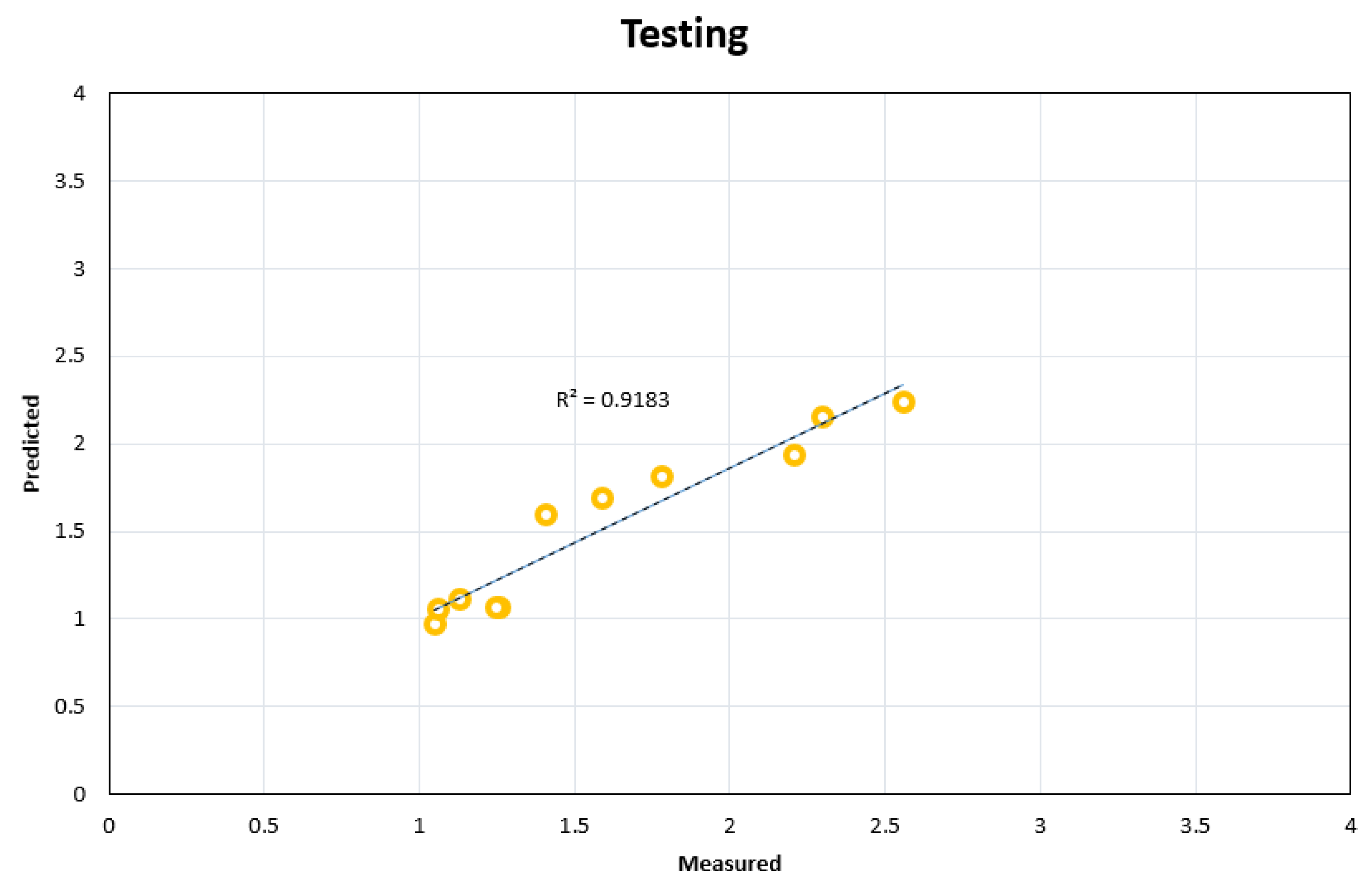
| GA-ANFIS | 0.9341 | 0. 129 | 0.9183 | 0.172 | Iteration (Generation) = 400 Population size = 40 | Crossover rate = 0.75 Mutation rate = 0.25 |
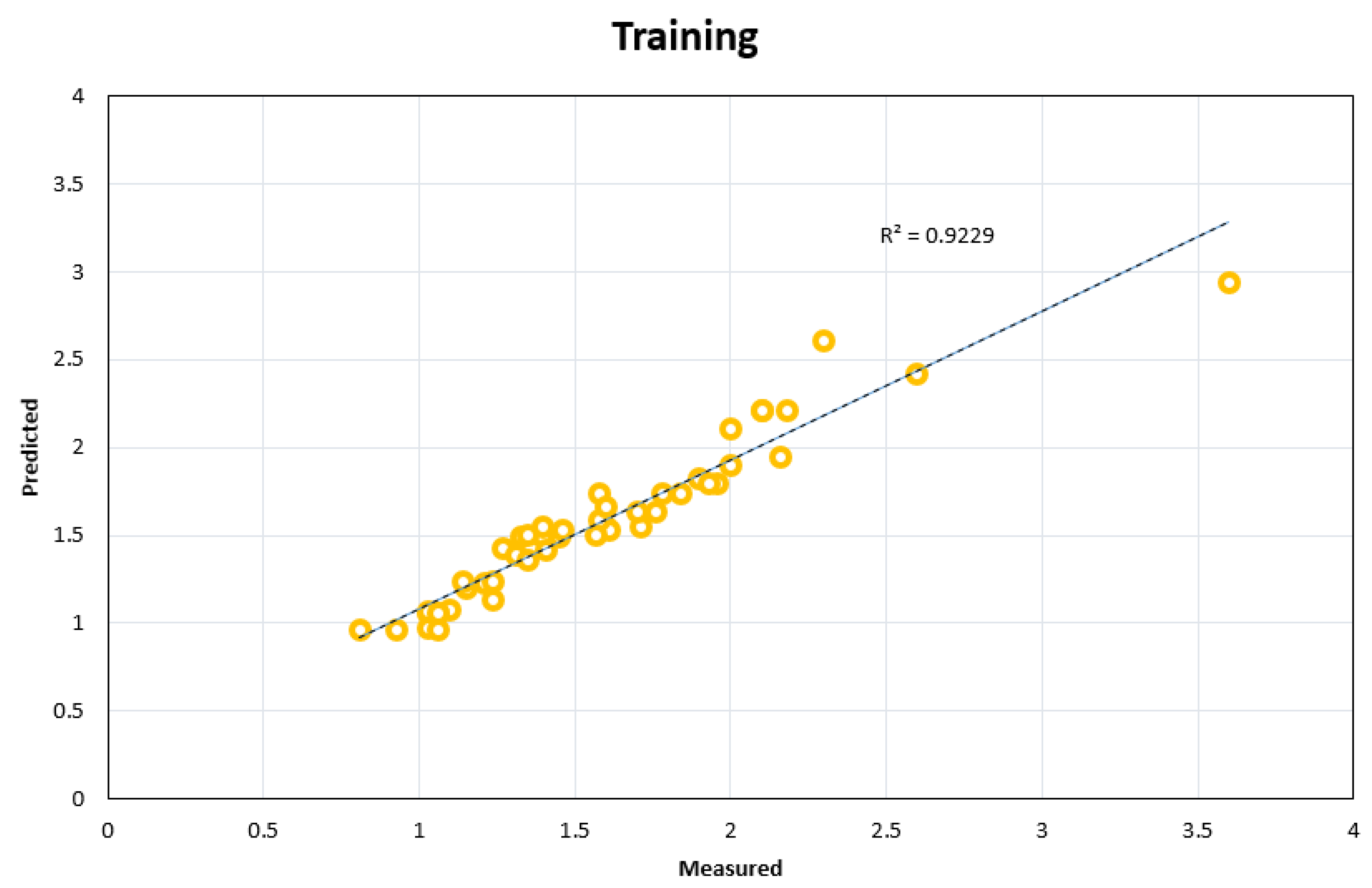
| PSO-ANFIS | 0.9229 | 0.144 | 0.9019 | 0.206 | Iteration = 400 Swarm size = 35 | Inertia coefficient = 0.75 Acceleration coefficients c1 = 2 and c2 = 2 |
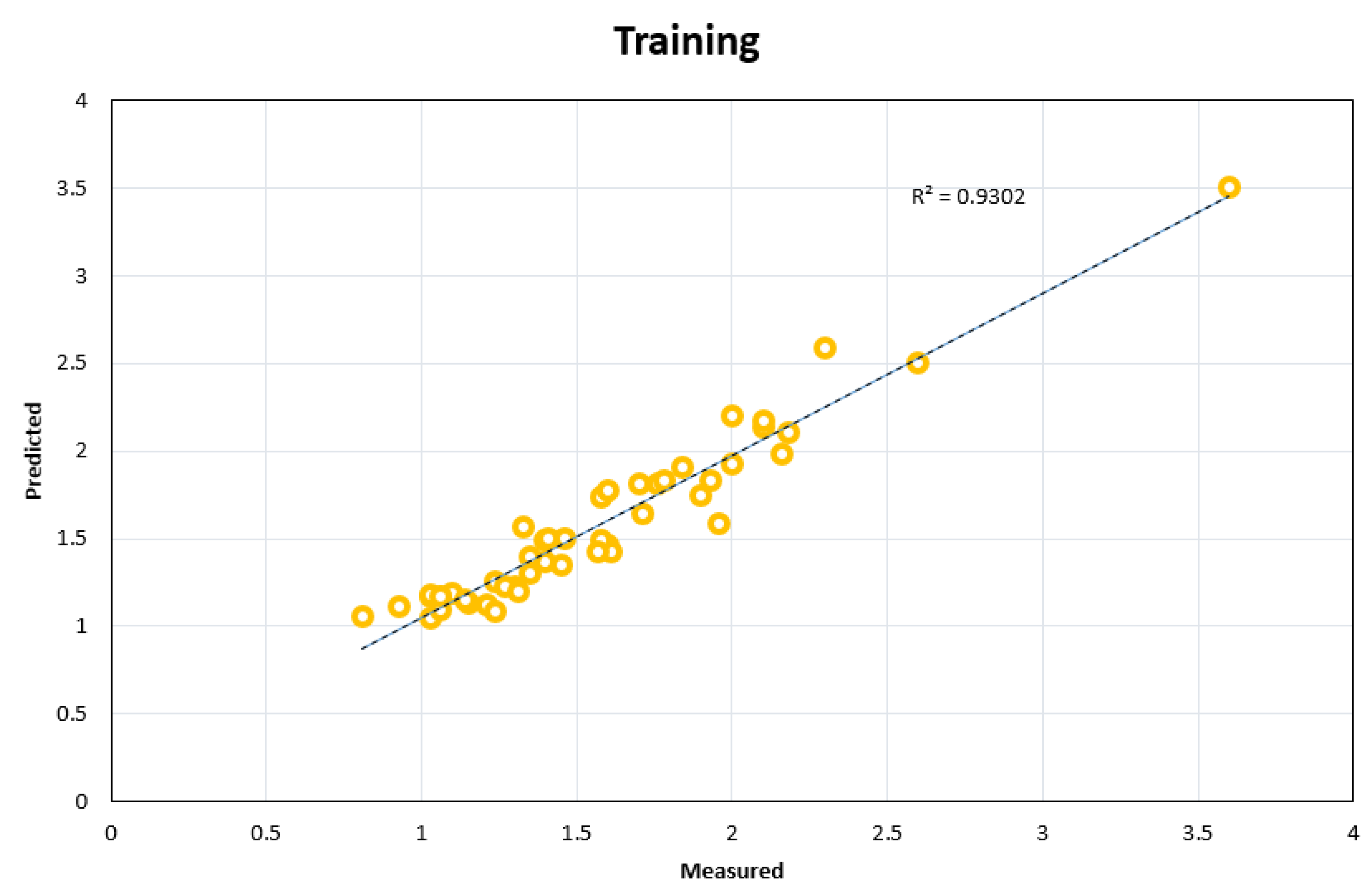
| ICA-ANFIS | 0.9302 | 0.132 | 0.9217 | 0.154 | Iteration (Ndecade) = 400 Ncountry = 30 Nimp = 10 | - |
| SDO-ANFIS | 0.9501 | 0.126 | 0.9449 | 0.134 | Iteration = 400 Market size = 35 | - |
Disclaimer/Publisher’s Note: The statements, opinions and data contained in all publications are solely those of the individual author(s) and contributor(s) and not of MDPI and/or the editor(s). MDPI and/or the editor(s) disclaim responsibility for any injury to people or property resulting from any ideas, methods, instructions or products referred to in the content. |
© 2022 by the authors. Licensee MDPI, Basel, Switzerland. This article is an open access article distributed under the terms and conditions of the Creative Commons Attribution (CC BY) license (https://creativecommons.org/licenses/by/4.0/).
Share and Cite
Cheng, G.; Lai, S.H.; Rashid, A.S.A.; Ulrikh, D.V.; Wang, B. Investigating the Effect of Parameters on Confinement Coefficient of Reinforced Concrete Using Development of Learning Machine Models. Sustainability 2023, 15, 199. https://doi.org/10.3390/su15010199
Cheng G, Lai SH, Rashid ASA, Ulrikh DV, Wang B. Investigating the Effect of Parameters on Confinement Coefficient of Reinforced Concrete Using Development of Learning Machine Models. Sustainability. 2023; 15(1):199. https://doi.org/10.3390/su15010199
Chicago/Turabian StyleCheng, Gege, Sai Hin Lai, Ahmad Safuan A. Rashid, Dmitrii Vladimirovich Ulrikh, and Bin Wang. 2023. "Investigating the Effect of Parameters on Confinement Coefficient of Reinforced Concrete Using Development of Learning Machine Models" Sustainability 15, no. 1: 199. https://doi.org/10.3390/su15010199