Macroeconomic Effects of COVID-19 Pandemic: Fresh Evidence from Korea

Abstract

Korea’s economy has suffered greatly as a result of the COVID-19 pandemic. Based on such a background, this paper investigates the macroeconomic effects of the COVID-19 pandemic. Via impulse response function analysis, the results reveal that the COVID-19 pandemic has a considerable short-term influence on Korea’s key macroeconomic variables, while its long-term effects are not significant. As a consequence of the COVID-19 pandemic, total demand in Korea has decreased. It is mostly reflected in the lower consumption and investment demand. Simultaneously, this has put increased pressure on inflation and unemployment. Moreover, the results also show that government investment expenditure and monetary policy may, to some degree, ameliorate the status of consumption demand. Meanwhile, they may alleviate employment pressures in order to boost output. In reality, both have some negative consequences. Based on the evidence presented in this article, the Korean government may implement appropriate policies to ensure the smooth functioning of the Korean macroeconomy.

1. Introduction

With the continued spread of the COVID-19 pandemic in Korea, it has had a major impact on many aspects of society, including people’s health and economic development. To curb the spread of the COVID-19 pandemic, Korea’s government has enacted laws requiring stores to shut early and limiting the number of people engaged in gathering activities. All of these COVID-19-fighting policies, however, will have an effect on Korea’s economy, such as consumption and total output [1]. The Korean government believes that the COVID-19 pandemic has caused the Korean economy to decline and that the worsening external environment has resulted in weak domestic demand and exports. A further drop in economic growth cannot be ruled out given the influence of the negative factors and the reappearance of the COVID-19 pandemic. Meanwhile, the COVID-19 pandemic has had a significant influence on Korea’s domestic demand. Specifically, the COVID-19 pandemic has significantly lowered the number of international visitors, slowed local demand, and reduced retail sales, dealing a more severe blow to Korea’s economy and society. In terms of domestic consumption, although the Korean government has not forced the closure of restaurants or shopping malls, the passenger flow through these establishments is often significantly smaller than it was before. Although supermarket and online shopping shipments have increased year over year as compared to physical shops, their profit margins have decreased significantly. Small- and medium-sized business owners often struggle when labor, shop leasing prices, and other expenditures are factored in. Of course, large enterprises have also been severely affected. In addition, in this COVID-19 pandemic situation, the investment and financial situation in Korea is bleak, and the possibility of firms acquiring financing at home and abroad, particularly abroad, is substantially diminished. Investor confidence has been significantly impacted as well. Many businesses’ investment plans have been thwarted, affecting the real economy and sectors in Korea’s various areas.

As a result, this article selects some representative macroeconomic variables in Korea to examine the influence of the COVID-19 pandemic on them in order to better deal with the macroeconomic impact of COVID-19 on Korea’s economy and assess the success of the Korean government’s strategies. We found that, in the short run, as a consequence of the effect of the COVID-19 pandemic, consumption and investment fell sharply, resulting in a drop in total output. Simultaneously, employment has fallen. Of course, these will lead to upward pressure on inflation. Furthermore, we also found that government investment expenditure and monetary policy may alleviate the COVID-19 pandemic’s impact on consumption and investment downward pressure, but they had some side-effects on Korea’s macroeconomic variables.

This paper contributes to the literature on the influence of COVID-19 on key macroeconomic variables in three ways. First, most Korean literature focuses on basic statistical data analysis to explain the economic effect of COVID-19 pandemic [2,3]. However, the dynamic stochastic general equilibrium model is used in this study to estimate the macroeconomic implications of the COVID-19 pandemic. This adds to the current body of knowledge, at least in terms of study methodologies. Secondly, the transparency of Korea’s COVID-19 policies might improve the accuracy and credibility of these empirical findings. Thirdly, government investment expenditure and monetary policy shocks are also discussed in this paper. The reason for this is that the influence of the COVID-19 pandemic on Korea’s key macroeconomic variables can be fully presented when compared to these two shocks.

The remainder of this paper is organized as follows: Section 2 examines the prior literature on this subject. The model is defined in Section 3. The findings are presented in Section 4. The last section presents the conclusions.

2. Literature Review

A great number of experts have recently emerged to examine the economic consequences of the COVID-19 pandemic. In this section, we review previous literature in terms of research techniques, research objectives, and research results in order to provide the theoretical groundwork for this article.

Walmsley et al. [4] used the United States as a case study to investigate the macroeconomic implications of mandated business closures to stop the spread of the COVID-19 pandemic. They created a new version of the global trade analysis project to conduct empirical studies. On an annual basis, their findings indicated a 20.3% drop in gross domestic product and a 22.4% drop in employment. Bairoliya and Imrohoroglu [5] employed the overlapping generation model with the same sample to examine the macroeconomic consequences of the COVID-19 pandemic. They discovered that the unexpected COVID-19 pandemic shock had a negative impact on total output, labor supply, savings, and consumption. Fernández-Villaverde and Jones [6] also examined the link between macroeconomic outcomes and COVID-19 pandemic. They discovered that the COVID-19 pandemic had reduced gross domestic product and employment. However, they also showed that the impact of the COVID-19 pandemic on the macroeconomies of Germany, Japan, Norway, and Korea is relatively modest when compared to other countries. These results were supported by Alvarez et al. [7] and Bigio et al. [8].

Malliet et al. [9] utilized the computed general equilibrium to investigate the economic impacts of the COVID-19 pandemic using France as a case study. They discovered that the COVID-19 pandemic assaults reduced production considerably, up to 5% of gross domestic product. Maliszewska et al. [10] used a similar technique to examine the probable impact of the COVID-19 pandemic on gross domestic product. They discovered that the COVID-19 pandemic reduced gross domestic product by 2% below the global average. Caggiano et al. [11] tried to assess the global impact of the COVID-19 pandemic. Empirical analysis was carried out using the vector auto-regression model. They discovered that the COVID-19 pandemic shock caused a 1.6% drop in global production. The total production loss over a year would be up to a 14%. McKibbin and Fernando [12] investigated seven different scenarios and macroeconomic outcomes for the COVID-19 pandemic using the global hybrid dynamic general stochastic equilibrium model and the computable general equilibrium model. The findings indicated that, even if the COVID-19 pandemic was contained, it might have a major effect on the world economy in the near future. Increased investment in public health systems, particularly in countries with less established health-care systems and high population density, might significantly reduce economic costs. Furthermore, Addison et al. [13] discovered that the COVID-19 pandemic had a detrimental impact on macroeconomic stability and growth. Moreover, Eichenbaum et al. [14] and Jones et al. [15] also agreed with findings above.

Zhao [16] aimed to explore the influence of the COVID-19 pandemic on macroeconomic variables using a sample of China by incorporating the Susceptible-Infectious-Recovered model into the Bewley-type incomplete market model. He discovered that, despite a decrease in the average tendency to use household wealth, there was an increase in the demand for money. He also discovered that an early abandoning of containment strategy caused a substantial reduction in both employment and production in the short term. Goswami et al. [17] used India as a case study to investigate the influence of the COVID-19 epidemic on macroeconomic performance. Using the panel regression model and monthly data from April to November 2020, they conducted empirical studies and discovered that the COVID-19 pandemic had a significant negative impact on economic growth in these states, particularly in the manufacturing and tertiary sectors. However, the effect of the COVID-19 epidemic on economic development was relatively modest in primary-industry-oriented countries. Jena et al. [18] employed an artificial neural network model to examine the economic effect of the COVID-19 pandemic in the United States, Germany, Spain, Italy, France, Japan, Mexico, and India. Their findings indicated that the shock of the COVID-19 pandemic caused a substantial reduction in gross domestic product during the second quarter of 2020. Boscá et al. [19] considered Spain to be a case study for analyzing the macroeconomic repercussions of the COVID-19 pandemic. Using a dynamic stochastic general equilibrium model to assess the Spanish economy, the yearly loss in gross domestic product was moderated by at least 7.6% points as a result of the COVID-19 pandemic shock. These results were consistent with Baqaee and Farhi [20], Eichenbaum et al. [21], and Guerrieri et al. [22].

Based on the aforementioned analyses, it can be concluded that, despite the fact that a large number of scholars have studied the effect of the COVID-19 pandemic on key macroeconomic variables using various samples and methods, their findings largely supported the idea that the COVID-19 pandemic had a negative effect on key macroeconomic variables such as output, consumption, and employment. However, as Korea is an import-and-export-oriented economy, its capacity to withstand the effect of COVID-19 is modest. Thus, using Korea as an example, the macroeconomic consequences of the COVID-19 pandemic may have diverse outcomes when compared to other countries. These findings may give policy suggestions to the Korean government in order to cope with the losses caused by the COVID-19 pandemic. At the same time, this article may contribute to the current literature on this subject.

3. Model

In this paper, COVID-19 pandemic is introduced into the new Keynesian framework. Following Gali and Jordi [23], the model includes three sectors: household, firm, and government. We attempt to simulate the COVID-19 pandemic on key macroeconomic indicators such as total output, consumption, investment, employment, inflation, wage, lending interest rate, price, and deposit interest rate, using Matlab and Dynare.

3.1. Household

Suppose that there is a representative household in the economic system. The utility function is given as follows:

$${\mathrm{E}}_0{{\displaystyle \sum }}_{\mathrm{t}=0}^{\infty }{\mathsf{\beta }}^{\mathrm{t}}\mathrm{U}({\mathrm{C}}_{\mathrm{t}},{\mathrm{N}}_{\mathrm{t}},\frac{{\mathrm{M}}_{\mathrm{t}}}{{\mathrm{P}}_{\mathrm{t}}}),$$

(1)

where ${\mathrm{C}}_{\mathrm{t}}$ denotes final goods consumption; ${\mathrm{N}}_{\mathrm{t}}$ denotes work house; ${\mathrm{M}}_{\mathrm{t}}$ denotes money holding; ${\mathrm{P}}_{\mathrm{t}}$ denotes price level; ${\mathrm{E}}_0$ denotes expectation operator; $\mathsf{\beta }$ denotes discount factor; $\mathrm{U}$ denotes utility function. Equation (1) is rewritten as follows:

$${\mathrm{Max}\mathrm{E}}_0{\displaystyle \sum }_{\mathrm{t}=0}^{\infty }{\mathsf{\beta }}^{\mathrm{t}}[{\mathrm{logC}}_{\mathrm{t}}-\frac{\mathsf{\theta }}{1+\mathsf{\theta }}{\mathrm{N}}_{\mathrm{t}}^{1+\mathsf{\theta }}+\frac{1}{1-\mathsf{\vartheta }}{(\frac{{\mathrm{M}}_{\mathrm{t}}}{{\mathrm{P}}_{\mathrm{t}}})}^{1-\mathsf{\vartheta }}]$$

(2)

where $\mathsf{\theta }$ denotes the inverse of labor elasticity; $\mathsf{\vartheta }$ denotes the inverse of real balance substitution elasticity. A representative household provides labor and capital to a firm. Meanwhile, a representative household also owns extra profits by holding money and bonds. The budget constraint of a representative household is given as follows:

P_tC_t + P_tI_t + B_t + M_t + T_t = W_tN_t + R_t¹K_t + (1 + R_t²)B_t−1 + D_t,

(3)

where I_t denotes investment; B_t denotes bonds; T_t denotes tax; W_t denotes wage; Rt¹ denotes interest rate for capital; K_t denotes capital; R_t² denotes interest rate for bonds; D_t denotes dividends. Suppose that there is an adjustment cost of investment. The law of capital motion is given as follows:

$${\mathrm{K}}_{\mathrm{t}+1}=\left(1-\mathsf{\delta }\right){\mathrm{K}}_{\mathrm{t}}+{\mathrm{I}}_{\mathrm{t}}[1-\frac{\mathsf{\chi }}{2}{\left(\frac{{\mathrm{I}}_{\mathrm{t}}}{{\mathrm{I}}_{\mathrm{t}-1}}\right)}^2],$$

(4)

where $\mathsf{\delta }$ denotes the capital depreciation rate; $\chi$ denotes the sensitivity parameter for the investment adjustment.

3.2. Firm

Suppose that there are two types of firms: one is the final goods production firm, and the other is the intermediate goods production firm. The former is subject to perfect competition, whereas the latter is subject to monopolistic competition.

3.2.1. Final Goods Production Firm

Suppose that there is a representative final goods production firm in the economy. Using production technology to produce the final goods (${\mathrm{Y}}_{\mathrm{t}}$), the expression is shown as follows:

$${\mathrm{Y}}_{\mathrm{t}}={[{{\displaystyle \int }}_0^1{\mathrm{Y}}_{\mathrm{t}}{\left(\mathrm{j}\right)}^{\frac{{\mathsf{\epsilon }}_{\mathrm{p}}-1}{{\mathsf{\epsilon }}_{\mathrm{p}}}}{\mathrm{d}}_{\mathrm{j}}]}^{\frac{{\mathsf{\epsilon }}_{\mathrm{p}}}{{\mathsf{\epsilon }}_{\mathrm{p}}-1}},$$

(5)

where ${\mathrm{Y}}_{\mathrm{t}}\left(\mathrm{j}\right)$ denotes intermediate goods produced by the jth intermediate goods production firm; ${\mathsf{\epsilon }}_{\mathrm{p}}$ denotes substitution elasticity between different intermediates.

Under the given production technology, the final goods price (${\mathrm{P}}_{\mathrm{t}}$) and the intermediate goods price (${\mathrm{P}}_{\mathrm{t}}\left(\mathrm{j}\right)$) of the final goods production firm are considered as given. The intermediate goods quantity (${\mathrm{Y}}_{\mathrm{t}}\left(\mathrm{j}\right)$) is selected to maximize the profit as follows:

$${}_{{\mathrm{Y}}_{\mathrm{t}}\left(\mathrm{j}\right)}{}^{\max }{\mathrm{P}}_{\mathrm{t}}{\mathrm{Y}}_{\mathrm{t}}-{{\displaystyle \int }}_0^1{\mathrm{P}}_{\mathrm{t}}{\mathrm{Y}}_{\mathrm{t}}\left(\mathrm{j}\right)\mathrm{dj}={\mathrm{P}}_{\mathrm{t}}{[{{\displaystyle \int }}_0^1{\mathrm{Y}}_{\mathrm{t}}{\left(\mathrm{j}\right)}^{\frac{{\mathsf{\epsilon }}_{\mathrm{p}}-1}{{\mathsf{\epsilon }}_{\mathrm{p}}}}]}^{\frac{{\mathsf{\epsilon }}_{\mathrm{p}}}{{\mathsf{\epsilon }}_{\mathrm{p}}-1}}-{{\displaystyle \int }}_0^1{\mathrm{P}}_{\mathrm{t}}\left(\mathrm{j}\right){\mathrm{Y}}_{\mathrm{t}}\left(\mathrm{j}\right)\mathrm{dj},$$

(6)

where the final goods production firm is subject to perfect competition. According to the classical assumption of perfect competition, its profit is zero. The nominal total output is shown as follows:

$${\mathrm{P}}_{\mathrm{t}}{\mathrm{Y}}_{\mathrm{t}}={{\displaystyle \int }}_0^1{\mathrm{P}}_{\mathrm{t}}\left(\mathrm{j}\right){\mathrm{Y}}_{\mathrm{t}}\left(\mathrm{j}\right)\mathrm{dj},$$

(7)

The determinant equation of total price level index is expressed as follows:

$${\mathrm{P}}_{\mathrm{t}}={[{{\displaystyle \int }}_0^1{\mathrm{P}}_{\mathrm{t}}{\left(\mathrm{j}\right)}^{1-{\mathsf{\epsilon }}_{\mathrm{p}}}]}^{\frac{1}{1-{\mathsf{\epsilon }}_{\mathrm{p}}}},$$

(8)

3.2.2. Intermediate Goods Production Firm

Suppose that the intermediate goods production firm uses the Cobb–Douglas production to produce goods. The function is given as follows:

$${\mathrm{Y}}_{\mathrm{t}}\left(\mathrm{j}\right)={\mathrm{A}}_{\mathrm{t}}{\mathrm{N}}_{\mathrm{t},\mathrm{co}}^{1-\mathsf{\gamma }}\left(\mathrm{j}\right){\mathrm{K}}_{\mathrm{t}}^{\mathsf{\gamma }}\left(\mathrm{j}\right){\mathrm{K}}_{\mathrm{t}}^{1\mathsf{\upsilon }}\left(\mathrm{j}\right),$$

(9)

where ${\mathrm{A}}_{\mathrm{t}}$ denotes the productivity; $\mathrm{j}$ denotes the $\mathrm{jth}$ firm; ${\mathrm{N}}_{\mathrm{t},\mathrm{co}}^{1-\mathsf{\gamma }}$ denotes the labor force affected by COVID-19 pandemic shock; ${\mathrm{K}}_{\mathrm{t}}^{1\mathsf{\upsilon }}$ denotes public capital; $\mathsf{\gamma }$ denotes the elasticity of the level of production with regard to capital; $\mathsf{\upsilon }$ denotes the elasticity of the level of production with regard to government investment expenditure.

In general, the effects of the COVID-19 pandemic on key macroeconomic variables are due to its effects on productivity and labor. Furthermore, the COVID-19 pandemic’s influence mechanism affects both households and firms by imposing distinct utility functions, budget constraints, and production functions. Following Lim [24], Lim [25], and Kaszowska-Mojsa and Wlodarczyk [26], total factor productivity is affected by two types of shocks. One is the technological advancement shock and the other is the COVID-19 pandemic shock.

The shocks are shown as follows:

$$\ln \frac{{\mathrm{A}}_{\mathrm{t}}}{\mathrm{A}}=\ln \frac{{\mathrm{a}}_{\mathrm{t}}}{\mathrm{a}}+\mathsf{\varsigma }\ln \frac{{\mathrm{co}}_{\mathrm{t}}}{\mathrm{co}},$$

(10)

where ${\mathrm{a}}_{\mathrm{t}}$ denotes the total factor productivity, which is not affected by COVID-19 productivity; ${\mathrm{co}}_{\mathrm{t}}$ denotes COVID-19 pandemic shock.

The labor force affected by COVID-19 pandemic shock is shown as follows:

$${\mathrm{N}}_{\mathrm{t},\mathrm{co}}\left(\mathrm{j}\right)={\mathrm{N}}_{\mathrm{t}}\left(\mathrm{j}\right)-{\mathsf{\varsigma }\mathrm{co}}_{\mathrm{t}}{\mathrm{N}}_{\mathrm{t}}\left(\mathrm{j}\right),$$

(11)

Suppose that the firm selects a labor and capital stock to minimize its costs:

$$\begin{array}{c}\min \\ {\mathrm{N}}_{\mathrm{t}}\left(\mathrm{j}\right),{\mathrm{K}}_{\mathrm{t}}\left(\mathrm{j}\right)\end{array}={\mathrm{W}}_{\mathrm{t}}{\mathrm{N}}_{\mathrm{t}}\left(\mathrm{j}\right)-{\mathrm{R}}_{\mathrm{t}}^1{\mathrm{K}}_{\mathrm{t}}\left(\mathrm{j}\right),$$

(12)

The budget constraint is shown as follows:

$${\mathrm{A}}_{\mathrm{t}}{\mathrm{N}}_{\mathrm{t},\mathrm{co}}^{1-\mathsf{\gamma }}\left(\mathrm{j}\right){\mathrm{K}}_{\mathrm{t}}^{\mathsf{\gamma }}\left(\mathrm{j}\right){\mathrm{K}}_{\mathrm{t}}^{\mathsf{\upsilon }}\left(\mathrm{j}\right)\ge {\mathrm{Y}}_{\mathrm{t}}\left(\mathrm{j}\right)={\left[\frac{{\mathrm{P}}_{\mathrm{t}}\left(\mathrm{j}\right)}{{\mathrm{P}}_{\mathrm{t}}}\right]}^{-{\mathsf{\epsilon }}_{\mathrm{p}}}{\mathrm{Y}}_{\mathrm{t}}=,$$

(13)

Then, the ratio between capital rent and wage is shown as follows:

$$\frac{{\mathrm{R}}_{\mathrm{t}}^1}{{\mathrm{W}}_{\mathrm{t}}}=\frac{\mathsf{\gamma }}{1-\mathsf{\gamma }}\frac{{\mathrm{N}}_{\mathrm{t},\mathrm{co}}\left(\mathrm{j}\right)}{{\mathrm{K}}_{\mathrm{t}}\left(\mathrm{j}\right)},$$

(14)

The real marginal cost is shown as follows:

$${\mathrm{M}}_{\mathrm{t}}={(\frac{1}{1-\mathsf{\gamma }})}^{1-\mathsf{\gamma }}{(\frac{1}{\mathsf{\gamma }})}^{\mathsf{\gamma }}\frac{1}{{\mathrm{A}}_{\mathrm{t}}}{\mathrm{K}}_{\mathrm{t}}^{1\left(-\mathsf{\upsilon }\right)}{(\frac{{\mathrm{W}}_{\mathrm{t}}}{{\mathrm{P}}_{\mathrm{t}}})}^{1-\mathsf{\gamma }}{(\frac{{\mathrm{R}}_{\mathrm{t}}^1}{{\mathrm{P}}_{\mathrm{t}}})}^{\mathsf{\gamma }},$$

(15)

where ${\mathrm{M}}_{\mathrm{t}}$ denotes real marginal cost.

3.2.3. Calvo Pricing

Because intermediate goods are differentiated, the intermediate goods production firm has an independent pricing power on their commodities in a market with monopolistic competition. Its goal is to maximize profits by setting a specified price. In this study, the nominal prices of the intermediate goods production firm in the economy is established in each period using a stochastic time-dependent rule defined by Calvo [27]. Specifically, a fraction of the intermediate goods production firm can establish a new pricing each time, while the others cannot be allowed to adjust their pricing (they will stick with the previous period’s price).

As a result, the cost of price adjustment is shown as follows:

$$\cos \mathrm{t}=\frac{\mathsf{\varpi }}{2}[\frac{{\mathrm{P}}_{\mathrm{t}}^{*}\left(\mathrm{j}\right)}{{\mathrm{P}}_{\mathrm{t}-1}^{*}\left(\mathrm{j}\right)}-1]{\mathrm{A}}_{\mathrm{t}}{\mathrm{N}}_{\mathrm{t},\mathrm{co}}^{1-\mathsf{\gamma }}\left(\mathrm{j}\right){\mathrm{K}}_{\mathrm{t}}^{\mathsf{\gamma }}\left(\mathrm{j}\right){\mathrm{K}}_{\mathrm{t}}^{1\mathsf{\upsilon }}\left(\mathrm{j}\right),$$

(16)

where $\mathsf{\varpi }$ denotes a percentage of intermediate goods production firms who can adjust their pricing. ${\mathrm{P}}_{\mathrm{t}}^{*}\left(\mathrm{j}\right)$ denotes the intermediate goods price.

The goal of the intermediate goods production firm is to establish a precise price that maximizes their predicted profits.

Predicted profits are shown as follows:

$${\mathrm{E}}_{\mathrm{t}}{\sum }_{\mathrm{i}=0}^{\infty }{\left(\mathsf{\beta }\mathsf{\theta }\right)}^{\mathrm{i}}{\mathsf{\lambda }}_{\mathrm{t}+\mathrm{i}}{\mathrm{P}}_{\mathrm{t}+\mathrm{i}}^{*}{\mathrm{Y}}_{\mathrm{t}+\mathrm{i}}\left(\mathrm{j}\right)-{\left(\mathsf{\beta }\mathsf{\theta }\right)}^{\mathrm{i}}{\mathsf{\lambda }}_{\mathrm{t}+\mathrm{i}}{\mathsf{\psi }}_{\mathrm{t}+\mathrm{i}}{\mathrm{Y}}_{\mathrm{t}+\mathrm{i}}\left(\mathrm{j}\right)-{\left(\mathsf{\beta }\mathsf{\theta }\right)}^{\mathrm{i}}{\mathsf{\lambda }}_{\mathrm{t}+\mathrm{i}}\frac{\mathsf{\theta }}{2}{[\frac{{\mathrm{P}}_{\mathrm{t}}^{*}}{{\mathrm{P}}_{\mathrm{t}-1}^{*}}-1]}^2{\mathrm{P}}_{\mathrm{t}+\mathrm{i}}^{*}\left(\mathrm{j}\right){\mathrm{Y}}_{\mathrm{t}+1}\left(\mathrm{j}\right)$$

(17)

where ${\left(\mathsf{\beta }\mathsf{\theta }\right)}^{\mathrm{i}}{\mathsf{\lambda }}_{\mathrm{t}+\mathrm{i}}$ denotes the discount rate of the future profits of intermediate goods production firms; ${\mathsf{\lambda }}_{\mathrm{t}}$ denotes the Lagrange multiplier of households’ budget constraint.

3.3. Government

Government uses the fiscal policy to regulate the key macroeconomic variables under the government budget constraint. The purpose is to maintain the output gap, government debt, and economic stability.

The government budget constraint is shown as follows:

$${\mathrm{T}}_{\mathrm{t}}+{\mathrm{B}}_{\mathrm{t}}=\left(1+{\mathrm{r}}_{\mathrm{t}-1}\right){\mathrm{B}}_{\mathrm{t}-1}+{\mathrm{G}}_{\mathrm{t}}^1+{\mathrm{G}}_{\mathrm{t}}^2,$$

(18)

where ${\mathrm{G}}_{\mathrm{t}}^1$ denotes government purchase; ${\mathrm{G}}_{\mathrm{t}}^2$ denotes government investment expenditure.

The public capital stock equation is shown as follows:

$${\mathrm{K}}_{\mathrm{t}}^{1\mathsf{\upsilon }}=\left(1-{\mathsf{\delta }}_2\right){\mathrm{K}}_{\mathrm{t}-1}^{1\mathsf{\upsilon }}+{\mathrm{G}}_{\mathrm{t}}^2,$$

(19)

where ${\mathsf{\delta }}_2$ denotes the depreciation rate.

The fiscal policy used to cope with external shocks in this study is government investment expenditure. As a result, if the macroeconomic system is hit by the COVID-19 pandemic, we would want to see how the government investment expenditure, which serves as a fiscal tool for macroeconomic operation, may be altered. Following Iwata [28], the government investment expenditure is shown as follows:

$$\frac{{\mathrm{G}}_{\mathrm{t}}^2}{{\mathrm{G}}^2}={(\frac{{\mathrm{G}}_{\mathrm{t}-1}^2}{{\mathrm{G}}^2})}^{\mathsf{\xi }}[{(\frac{{\mathrm{Y}}_{\mathrm{t}}}{\mathrm{Y}}{)}^{-\varrho }]}^{-\mathsf{\xi }}{\mathsf{\mu }}_{\mathrm{t}}^1,$$

(20)

where ${\mathsf{\mu }}_{\mathrm{t}}^1$ denotes government investment expenditure shock. This shock is defined as an independent and identically distributed normal error term.

3.4. Central Bank

The central bank may exert control over the monetary policy by establishing the nominal interest rate in accordance with the Taylor (1993) rule. It is shown as follows:

$$\frac{{\mathrm{R}}_{\mathrm{t}}^1}{{\mathrm{R}}^1}={(\frac{{\mathrm{R}}_{\mathrm{t}-1}^1}{{\mathrm{R}}^1})}^{{\mathsf{\rho }}_{\mathrm{r}}}\{{(\frac{{{{\displaystyle \prod }}^{}}_{\mathrm{t}}}{{{\displaystyle \prod }}^{}})}^{{\mathsf{\theta }}_{\mathsf{\pi }}}{[\frac{\frac{{\mathrm{Y}}_{\mathrm{t}}}{\mathrm{Y}}}{\frac{{\mathrm{Y}}_{\mathrm{t}-1}}{\mathrm{Y}}}]}^{{\mathsf{\theta }}_{\mathrm{y}}}\}{\mathsf{\mu }}_{\mathrm{t}}^2,$$

(21)

where ${\mathsf{\rho }}_{\mathrm{r}}$ denotes the degree of interest-rate smoothing; ${\mathsf{\theta }}_{\mathsf{\pi }}$ denotes weights the central bank places on inflation; ${\mathsf{\theta }}_{\mathrm{y}}$ denotes weights the central bank places on the output gap; ${\mathsf{\mu }}_{\mathrm{t}}^2$ denotes the monetary policy shock that is defined as an independent and identically distributed normal error term.

3.5. Market Clearing

Goods market clearing conditions require aggregate output to be equal to aggregate demand.

$${\mathrm{Y}}_{\mathrm{t}}={\mathrm{C}}_{\mathrm{t}}+{\mathrm{I}}_{\mathrm{t}}+{\mathrm{G}}_{\mathrm{t}}^1+{\mathrm{G}}_{\mathrm{t}}^2,$$

(22)

The bonds market is shown as follows:

$${\mathrm{B}}_{\mathrm{t}}=0,$$

(23)

4. Results and Discussion

4.1. Parameters

The parameters in this study are determined using two approaches. The first approach is to estimate the parameters using Bayesian Estimation. The second approach is to calibrate the parameters.

4.1.1. Bayesian Estimation

The Economic Statistics System of the Bank of Korea provides quarterly data for the period Q1 2000–Q1 2021. Two variables (South Korea’s GDP and deposit interest rate) are used in this study. This paper pertains to Choi’s [29] processing approach, which deals with both raw and processed data. Both variables are taken into the logarithm to eliminate both data trends. Then, the two investigated variables are taken as the first difference. After that, they are multiplied by 100. To be calculated, the total number of observations are up to 81.

For Bayesian estimation, let $\mathrm{p}\left({\mathsf{\theta }}_{\mathrm{M}}|\mathrm{M}\right)$ indicate the prior distribution of the parameter vector ${\mathsf{\theta }}_{\mathrm{M}}$ for some model. Let the likelihood function of the observed data conditional on the model and its parameters be represented by $\mathrm{L}\left({\mathsf{\theta }}_{\mathrm{M}}{|\mathrm{Y}}_{\mathrm{T}},\mathrm{M}\right)\equiv \mathrm{p}\left({\mathrm{Y}}_{\mathrm{T}}{|\mathsf{\theta }}_{\mathrm{M}},\mathrm{M}\right)$. Here, $\mathrm{p}\left({\mathrm{Y}}_{\mathrm{T}}{|\mathsf{\theta }}_{\mathrm{M}},\mathrm{M}\right)$ is the density of the data, and $\mathrm{Y}$ denotes observations until period $\mathrm{T}$. $\mathrm{p}(·)$ stands for the probability density function (pdf), e.g., gamma, beta, generalized beta, normal, inverse gamma, shifted gamma, and uniform function [30]. Let the marginal density function of the data conditional on the model be written as:

$$\mathrm{p}\left({\mathrm{Y}}_{\mathrm{T}}|\mathrm{M}\right)={{\displaystyle \int }}_{{\mathsf{\theta }}_{\mathrm{M}}}^{⬚}\mathrm{p}\left({\mathsf{\theta }}_{\mathrm{M}},{\mathrm{Y}}_{\mathrm{T}}|\mathrm{M}\right){\mathrm{d}\mathsf{\theta }}_{\mathrm{M}}={{\displaystyle \int }}_{{\mathsf{\theta }}_{\mathrm{M}}}^{⬚}\mathrm{p}\left({\mathrm{Y}}_{\mathrm{T}}{|\mathsf{\theta }}_{\mathrm{M}},\mathrm{M}\right)\mathrm{p}\left({\mathsf{\theta }}_{\mathrm{M}}|\mathrm{M}\right){\mathrm{d}\mathsf{\theta }}_{\mathrm{M}}$$

(24)

Then, using Bayes theorem, the posterior density $\mathrm{p}\left({\mathsf{\theta }}_{\mathrm{M}}{|\mathrm{Y}}_{\mathrm{T}},\mathrm{M}\right)$ can be expressed as the product of the likelihood function and the prior density:

$$\mathrm{p}\left({\mathsf{\theta }}_{\mathrm{M}}{|\mathrm{Y}}_{\mathrm{T}},\mathrm{M}\right)=\frac{\mathrm{p}\left({\mathrm{Y}}_{\mathrm{T}}{|\mathsf{\theta }}_{\mathrm{M}},\mathrm{M}\right)\mathrm{p}\left({\mathsf{\theta }}_{\mathrm{M}}|\mathrm{M}\right)}{\mathrm{p}\left({\mathrm{Y}}_{\mathrm{T}}|\mathrm{M}\right)},$$

(25)

$$\mathrm{p}\left({\mathsf{\theta }}_{\mathrm{M}}{|\mathrm{Y}}_{\mathrm{T}},\mathrm{M}\right)=\frac{\mathrm{L}\left({\mathsf{\theta }}_{\mathrm{M}}{|\mathrm{Y}}_{\mathrm{T}},\mathrm{M}\right)\mathrm{p}\left({\mathsf{\theta }}_{\mathrm{M}}|\mathrm{M}\right)}{{{\displaystyle \int }}_{{\mathsf{\theta }}_{\mathrm{M}}}^{⬚}\mathrm{p}\left({\mathrm{Y}}_{\mathrm{T}}{|\mathsf{\theta }}_{\mathrm{M}},\mathrm{M}\right)\mathrm{p}\left({\mathsf{\theta }}_{\mathrm{M}}|\mathrm{M}\right){\mathrm{d}\mathsf{\theta }}_{\mathrm{M}}},$$

(26)

The posterior kernel corresponds to the numerator of the posterior density, given as $\mathrm{k}\left({\mathsf{\theta }}_{\mathrm{M}}{|\mathrm{Y}}_{\mathrm{T}},\mathrm{M}\right)\equiv \mathrm{L}\left({\mathrm{Y}}_{\mathrm{T}}{|\mathsf{\theta }}_{\mathrm{M}},\mathrm{M}\right)\mathrm{p}\left({\mathsf{\theta }}_{\mathrm{M}}|\mathrm{M}\right)$. The posterior distribution of the parameter vector ${\mathsf{\theta }}_{\mathrm{M}}$ for model $\mathrm{M}$ is directly proportional to the posterior density. This can be written as:

$$\mathrm{p}\left({\mathsf{\theta }}_{\mathrm{M}}{|\mathrm{Y}}_{\mathrm{T}},\mathrm{M}\right)\propto \mathrm{L}\left({\mathsf{\theta }}_{\mathrm{M}}{|\mathrm{Y}}_{\mathrm{T}},\mathrm{M}\right)\mathrm{p}\left({\mathsf{\theta }}_{\mathrm{M}}|\mathrm{M}\right),$$

(27)

The above distribution is characterized by: standard measures of central tendency, such as the mean, mode, or median; and measures of dispersion, such as the standard deviation, or some selected percentiles. When the model and data of observations are given, the likelihood function can be calculated using the Kalman filter or other particle filters for nonlinear models.

As part of this study, Bayesian estimation is used to find the parameters. Because of this, both the prior mean and prior distribution must be given. Following Takyi and Leon-Gonzalez [31], the prior mean of government investment expenditure smoothing is 0.886 with a beta distribution. Following Choi [29], the prior mean of the output gap is 0.500 with a gamma distribution. Following Hwang [32], and Yie and Yoo [33], the prior mean of degree of interest-rate smoothing is 0.750 with a beta distribution. Following Yie and Yoo [33], the prior mean of weights the central bank places on inflation is 1.700 with a gamma distribution. Following Hwang [32], and Yie and Yoo [33], the prior mean of weights the central bank places on output growth is 0.500 with a gamma distribution. Following Jeong [34], the prior mean of capital depreciation rate is 0.025 with a beta distribution. Following Takyi and Leon-Gonzalez [31], the prior mean of government investment expenditure is 0.500 with an inverse gamma distribution. Following Takyi and Leon-Gonzalez [31], the prior mean of benchmark interest is 0.700 with an inverse gamma distribution. Following Junior et al. [35], the prior mean of COVID-19 is 0.500 with an inverse gamma distribution. The results of Bayesian estimation are shown in

Table 1. Results of Bayesian estimation.

Parameter	Definition	Prior Mean	Posterior Mean	95% HPD Interval		Prior Distribution	Posterior Deviation
$\mathsf{\xi }$	Government investment expenditure smoothing	0.886	0.869	0.868	0.882	Beta	0.010
$\mathsf{\rho }$	output gap	0.500	0.498	0.482	0.516	Gamma	0.010
${\mathsf{\rho }}_{\mathrm{r}}$	Degree of interest-rate smoothing	0.750	0.750	0.746	0.753	Beta	0.010
${\mathsf{\theta }}_{\mathsf{\pi }}$	Weights the central bank places on inflation	1.700	2.514	2.248	2.774	Gamma	0.010
${\mathsf{\theta }}_{\mathrm{y}}$	Weights the central bank places on output growth	0.500	0.498	0.497	0.504	Gamma	0.010
$\mathsf{\delta }$	Capital depreciation rate	0.025	0.006	0.002	0.011	beta	0.010
${\mathrm{e}}_1$	Government investment expenditure shock	0.500	0.502	0.564	0.644	inverse gamma	0.200
${\mathrm{e}}_1$	Benchmark interest shock	0.700	0.846	0.790	0.886	inverse gamma	0.200
${\mathrm{e}}_1$	COVID-19 shock	0.500	0.740	0.598	0.894	inverse gamma	0.200

.

4.1.2. Parameter Calibration

The parameters utilized in this subsection are taken from prior significant research publications in the field. Furthermore, this study makes as many references to pertinent South Korean literature as feasible. The reason is that the fundamental features of South Korea’s real economic activity may then be properly expressed. Following Yoo [36], the inverse of the real balance substitution elasticity is 1.250. Following Jeong [34], the inverse of labor elasticity is 1.093. Following Yie and Yoo [33], the sensitivity parameter for investment adjustment is 0.971. Following Rhee [37], and Yie and Yoo [33], the elasticity of substitution between differentiated goods is 6.000. Following Kim et al. [38], the elasticity of the level of production with regard to capital is 0.450. Following Takyi and Leon-Gonzalez [31], the elasticity of the level of participation of capital with regard to government spending is 0.200. Following Rhee [37], and Yie and Yoo [33], the proportion of intermediate goods production firms who can adjust their price is 0.750. Following Kim et al. [38], and Yie and Yoo [33], the subjective discount factor is 0.990. Following Takyi and Leon-Gonzalez [31], the public capital depreciation rate is 0.020. The results of parameter calibration are shown in

Table 2. Results of parameter calibration.

Parameter	Value	Definition	Source
$\mathsf{\theta }$	1.250	Inverse of real balance substitution elasticity	Yoo [36]
$\mathsf{\vartheta }$	1.093	Inverse of labor elasticity	Jeong [34]
$\mathsf{\chi }$	0.971	Sensitivity parameter for investment adjustment	Yie and Yoo [33]
${\mathsf{\epsilon }}_{\mathrm{p}}$	6.000	Elasticity of substitution between differentiated goods	Rhee [37]; Yie and Yoo [33]
$\mathsf{\gamma }$	0.450	Elasticity of the level of production with regard to capital	Kim et al. [38]
$\mathsf{\upsilon }$	0.200	Elasticity of the level of participation of capital with regard to government spending	Takyi and Leon-Gonzalez [31]
$\mathsf{\varpi }$	0.750	Proportion of intermediate goods production firms who can adjust their price	Rhee [37]; Yie and Yoo [33]
$\mathsf{\beta }$	0.990	Subjective discount factor	Kim et al. [38]; Yie and Yoo [33]
${\mathsf{\delta }}_2$	0.020	Public capital depreciation rate	Takyi and Leon-Gonzalez [31]

.

4.2. Impulse Response Function Analysis

The implications of the COVID-19 pandemic, government investment expenditure, and monetary policy shocks on South Korea’s key macroeconomic variables including output, consumption, investment, employment, inflation, wages, lending interest rate, price level, and deposit interest rate are explored extensively in this subsection. These key macroeconomic variables are simulated by the Dynare 4.6.2 version based on Matlab. Furthermore, the dynamic reactions of these variables represent a standard deviation shock to all innovations. Meanwhile, they provide a percentage-point variation from their steady state. Furthermore, the mean impulse response is shown by the black line in bold, whereas the steady state is represented by the red line. One by one, these three types of shocks are simulated and examined in the following sections.

4.2.1. COVID-19 Pandemic Shock

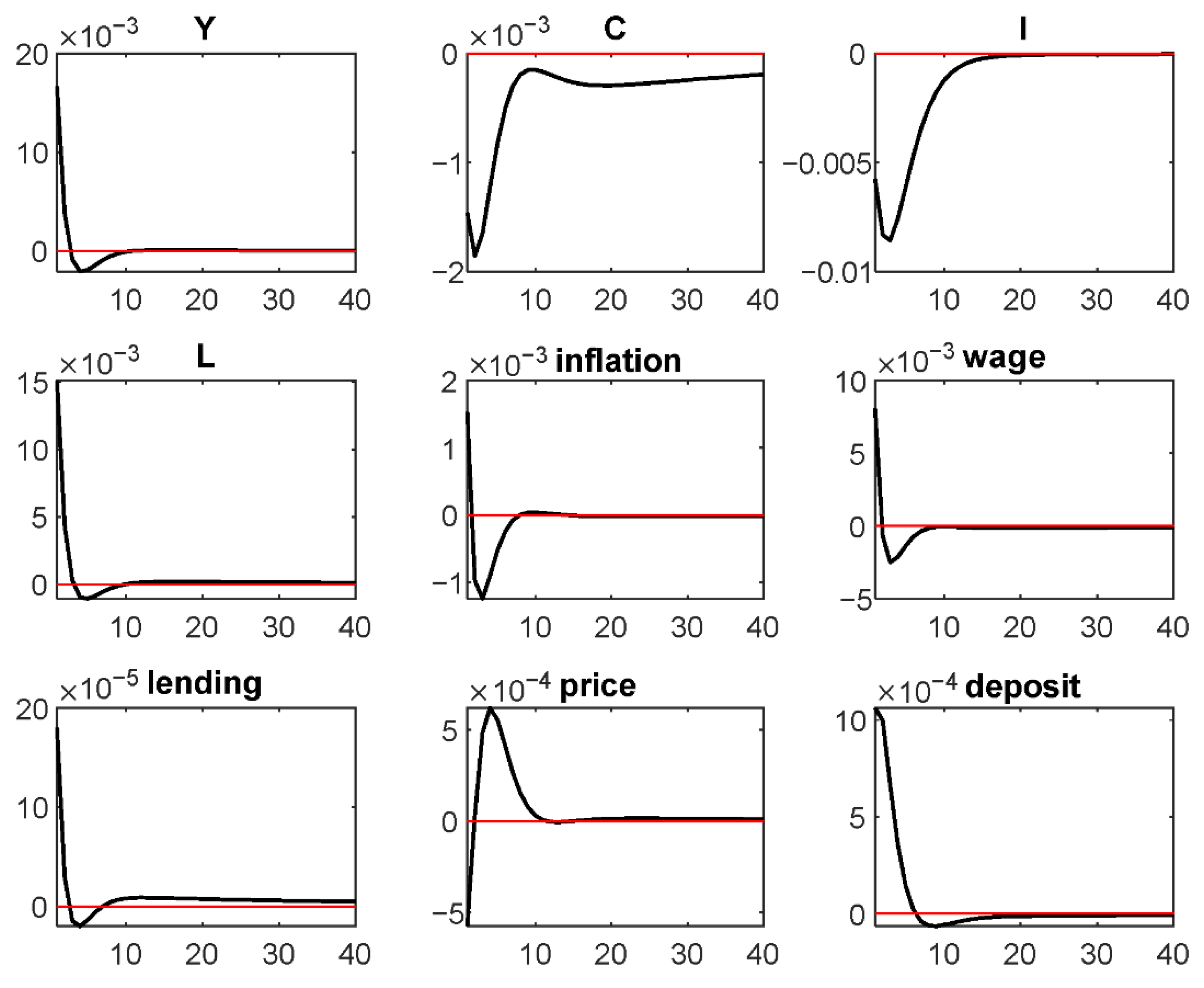
Following McKibbin and Fernando [39], and Adam et al. [40], the shock of the COVID-19 pandemic has caused significant changes in macroeconomic variables. This subsection simulates the effects of COVID-19 on Korea’s key macroeconomic variables. The results are shown in Figure 1.

Figure 1 shows the results of effects of the COVID-19 pandemic on Korea’s macroeconomic variables including total output, consumption, investment, work hours, inflation, wage, lending interest rate, price level, and deposit interest rate. It can be seen that, as a result of the shock of the COVID-19 pandemic, the total output instantly decreases from positive to negative. One probable reason is that, in order to comply with the government’s COVID-19 pandemic-fighting-policies, which prohibits people from gathering, businesses have to reduce their output size or possibly shut down. Furthermore, it is shown that both consumption and investment decrease as a consequence of the COVID-19 pandemic shock. These phenomena might be explained by two factors. The first reason is that a decreased total output leads to decreased consumption and investment. The second reason is that decreased mobility as a consequence of the COVID-19 pandemic leads to less activities. As a result, the consumption decreases. Simultaneously, the need for investment is decreasing. Furthermore, enterprises’ routine manufacturing operations are disrupted, resulting in a short-term supply shortage. As a result, inflation will arise in the short term. Likewise, as a result of the short-run economic slowdown induced by the shock of the COVID-19 pandemic, labor market demand will tighten, resulting in a decrease in employment. Of course, in the short term, the wage increases instantly and then stabilizes. Meanwhile, in order to reduce enterprises’ short-term debts, the central bank will lower loan interest rates in the short run. The price will decline in the short run to boost short-run demand and stabilize the market. In terms of the deposit interest rate, there are two possible explanations. On the one hand, by hiking the deposit interest rate, the government may generate more funds to combat the COVID-19 pandemic. Raising the deposit interest rate, on the other hand, might be seen as a kind of transfer payment for households to compensate for the loss created by unemployment. In summary, the effects of the COVID-19 pandemic on Korea’s key macroeconomic variables, with the exception of consumption, will vanish in the long run.

4.2.2. Government Investment Expenditure and Monetary Policy Shocks

As the COVID-19 pandemic spread, the Korean government implemented fiscal and monetary measures to mitigate the COVID-19 pandemic’s effects on the macroeconomy. The results of the effects of government investment expenditure and monetary policy on Korea’s macroeconomic variables are shown in Figure 2 and Figure 3.

According to the findings in Figure 2, an exogenous increase in government investment expenditure will result in a temporary increase in output and employment. They will drop for a short time before returning to their previous level. Because of the uncertainty in the investment market and the constraints on private consumption, when government investment expenditure is increased exogenously, both investment and consumption would decline. Due to the general reduction in supply, both inflation and wages are expected to rise in the short term. In reality, they will implement certain associated rules to control this kind of tendency. As a result, with a small drop, both of them will return to their steady state. Meanwhile, wages respond in the same way as employment does when the government investment expenditure shock occurs. According to the Phillips curve, inflation will follow the same pattern as the price. Because of the government investment expenditure shock during the COVID-19 pandemic, both consumption and investment fall. As a result, both the deposit and lending interest rates climb. To summarize, the government investment expenditure shock to consumption and lending interest rates is sustained.

Then, we turn to the effects of monetary policy on Korea’s macroeconomic variables. The results are shown in Figure 3.

Because interest plays a role in monetary policy behavior, Figure 3 shows the responses of key macroeconomic variables to the monetary policy shock. The response of the output will be negative as a result of a standard deviation monetary expansion, and it will revert to a steady state. The labor market therefore responds to the drop in total output first. As a result, employment falls. The wage will fall as a result of the employment supply function. Meanwhile, inflation will fall as a result of the Phillips curve. The price will then rise. Furthermore, a drop in wages will result in a drop in consumption. Furthermore, a drop in total output leads to a decline in investment. A decrease in investment, according to the investment function, will result in an increase in the deposit interest rate. In reality, the loan interest rate will fall in order to alleviate enterprises’ loan burdens. Only one of the responses to consumption and the loan interest rate may be sustained as a result of the monetary shock.

5. Conclusions

The COVID-19 pandemic has a significant influence on people’s lives and health, as well as on Korea’s macroeconomic operation. Therefore, this study investigates the influence of the COVID-19 pandemic on Korea’s key macroeconomic variables, including total output, consumption, investment, employment, inflation, wages, loan interest rate, price, and deposit interest rate. The results of impulse response function analysis show that the COVID-19 pandemic reduces total output, consumption, investment, employment, price level, and loan interest rates, while it increases inflation, wage, and deposit interest rates in the short run. Specifically, according to the pattern of economic development, the macroeconomic effects of the COVID-19 pandemic are phased, and its long-term effects are insignificant. The total demand for the Korean economy has decreased because of the COVID-19 pandemic shock. This is mostly seen in a contraction in consumption and investment demand. At the same time, inflation and unemployment are on the rise. This is mostly due to a significant drop in production factors (labor force) and an increase in production costs. Under the impact of the COVID-19 pandemic, government investment expenditure and monetary policy can alleviate the pressure on employment and increase output to some extent, but investment expenditure has a crowding out effect on social capital, and monetary policy is accompanied by longer-term inflationary pressure.

This work contributes to the Korean literature in several aspects. First, this paper uses the dynamic stochastic general equilibrium model and Bayesian estimation instead of the basic statistical data analysis to explore the macroeconomic effects of the COVID-19 pandemic. Secondly, because of the transparency of Korea’s COVID-19-fighting-policies and the timeliness of COVID-19 pandemic reporting, using Korea as the study object to investigate the macroeconomic impacts of the COVID-19 pandemic is more reasonable. Thirdly, government investment expenditure and monetary policy are introduced in this paper to explore the macroeconomic effects of the COVID-19 pandemic. These three points may enrich the Korean literature to some extent.

This study proposes some policy implications based on the findings of the empirical investigation shown above. With the COVID-19 pandemic under control, enterprises resume manufacturing and economic activities return to normality. To support economic recovery more effectively and quickly, we propose using the essential function of monetary policy to lower the deposit reserve ratio, which injects liquidity into the market. Moreover, we also recommend increasing government investment, creating new investment channels, and enhancing investment efficiency. Finally, we suggest that the government directly provide financial assistance to the populations most impacted by the COVID-19 pandemic, particularly those in need of basic living necessities.

Of course, there are several limitations in this article, which also suggests some potential research areas for future scholars. First, the COVID-19 pandemic has had a significant influence on the import and export sector. It is advised that future studies take the import and export sector into consideration to examine the macroeconomic consequences of the COVID-19 pandemic. Secondly, the financial sector is especially crucial in the battle against the COVID-19 pandemic, but it is equally susceptible to the COVID-19 pandemic’s consequences. As a result, future scholars may supplement this article with information from the financial sector.