Stochastic Second-Order Conic Programming for Optimal Sizing of Distributed Generator Units and Electric Vehicle Charging Stations

Abstract

The increased penetration of electric vehicles (EVs) and distributed generator (DG) units has led to uncertainty in distribution systems. These uncertainties—which have not been adequately considered in the literature—can entail risks in the optimal sizing of EV charging stations (EVCSs) and DG units in active distribution network planning. This paper proposes a method for obtaining the optimal sizing of DG units and EVCSs (considering uncertainty), to achieve exact power system analysis and ensure EV driver satisfaction. To model uncertainties in optimal sizing planning, this study first generates scenarios for each system asset using a probability distribution that considers the asset characteristics. In this step, the wind-turbine (WT), PV, and EVCS are modeled applying the Weibull, exponential, and kernel density estimation (KDE), and scenarios for each asset are generated using random sampling. Then, the k-means clustering is carried out for scenario reduction and the representative scenario abstract. The probability of occurrence for each representative scenario is assigned depending on the number of observations within each cluster. The representative scenarios for each asset are integrated into the scenario for all assets through the joint probability. The integrated scenarios are applied in the optimization problem for optimal sizing of the system asset framework. The optimal sizing of the system assets problem is proposed (to minimize the line loss and voltage deviation) and formulated via stochastic second-order conic programming, to reflect the uncertainty under an AC power flow; this is a convex problem that can be solved in polynomial time. The proposed method is tested on a modified IEEE 15 bus system, and the simulation is performed with various objective functions. The simulation results demonstrate the effectiveness of the proposed method.

1. Introduction

1.1. Motivation

Concerns over climate change and the recent developments in technology have caused distributed generation (DG) and electric vehicles (EVs) to attract worldwide attention as eco-friendly alternatives to fossil fuel-based power plants [1]. In an active distribution network (ADN) that integrates a combination of DG units and EV charging stations (EVCSs), uncertainties arising from the high penetration of DG units and EVs in the distribution systems cause challenges for the distribution system operator (DSO) [2,3]. The increase in DG units (e.g., photovoltaic (PV) and wind-turbine (WT)) leads to uncertainty on the supply side, whilst increasing EV penetration leads to uncertainty on the demand side. Therefore, the optimal sizing framework of system assets in the distribution planning should consider these uncertainties. Since the EVCS uncertainty does not follow specific probability distribution (e.g., normal, exponential distribution) that is a parametric method, asset characteristics should be adequately modeled. If not, cost losses and lower utilization rates may arise through the oversizing of system assets. Meanwhile, the optimal capacity of each asset (i.e., PV, WT, and EVCS) should be optimized to satisfy driver convenience and system constraints (e.g., voltage and permitted current). For the accurate analysis of power systems, power flow should be applied in the distribution planning model. However, AC power flow is generally nonconvex and NP-hard due to its nonlinear nature, thus making the optimization problem challenging. To this end, the DC power flow is widely used, which is a popular approximation and a linearization of AC power flow [4,5,6,7]. DC power flow makes the optimization problem easy to solve and is based on some assumptions [8]: (1) The line resistance can be neglected because the reactance is much larger than the resistance in the transmission system. (2) The bus voltages are fixed as 1.0 pu These assumptions are valid in the transmission system but not in the distribution system because the R/X ratio cannot be ignored as in the transmission system. Furthermore, the bus voltage is the main issue in the distribution system. Therefore, the AC power flow should be applied in the AND planning, and it can be solved using the metaheuristics method, which does not ensure the global optimum.

1.2. Literature Review

Numerous studies in the literature have addressed these challenges, by placing various requirements upon the optimal sizing problem. In [9], a review of the systematic modeling and analysis of EVs integrated hybrid renewable energy system is presented. In [10], the EVCS sizing framework was introduced by incorporating the different types of EVCS (e.g., public parking lot and roadside fixed charging stations) into an NP-hard problem. This was solved by a Voronoi diagram-based particle swarm optimization. In [11], optimal storage and DG planning were formulated to reflect the uncertainty of EVs. This problem was solved using tabu search and simulated annealing algorithms for short-term and long-term planning, respectively. The authors of [12,13] sought to minimize the net present value of the total cost. In [12], the optimal sizing of the DGs and an energy storage system (ESS) was formulated using mixed-integer linear programming (MILP). In [13], the model predictive control-based optimization model for EVCS planning was formulated as a second-order conic program (SOCP), to minimize the system operation cost. Meanwhile, several researchers have performed optimizations to minimize power system loss or voltage deviations [14,15,16]. The authors in [14] aimed to minimize the power loss and maximize the penetration of system assets. For system loss analysis, AC power flow was applied, and SOCP relaxation was performed. In [15], an optimization model for EVCS sizing was proposed and solved using particle swarm optimization and a genetic algorithm (GA), to minimize power loss. Similarly, [16] proposed multi-objective EV charging station planning with the aim of minimizing the power loss and voltage deviation. Furthermore, the optimization problem for distribution assets (e.g., transformers and feeders) and DG units was modeled as an MILP in [12]. The authors of [2] proposed the joint planning of PVs, micro-turbines, and an EVCS for cost minimization. However, these studies were based on point optimization, which does not consider uncertainty. From a practical point of view, performing optimal sizing without considering this uncertainty may lead to the above-mentioned oversizing. Although a typical day from each season was applied in [2], it is difficult to ascertain whether uncertainty was fully considered. Moreover, power system constraints were neglected in [10,12], and most of these studies did not fully consider PVs, WTs, or EVCS.

The optimal sizing of system assets should consider the uncertainty of those assets; therefore, several researchers have conducted scenario-based optimizations such as stochastic programs and chance-constrained programs (CCPs). The authors of [17] proposed a CCP-based method for the optimal sizing of DGs; they considered the uncertainty of EVs, electricity prices, and DGs via a probability distribution function (PDF), and they solved the problem using a GA. In [3,10,18], a stochastic mixed-integer nonlinear program was formulated to reflect the uncertainty, and AC power flow was applied to each optimization model. The model for [3] aimed to minimize the investment cost, energy loss, and waiting time of EVCSs in a sharing EV system; it was solved by a natural aggregation algorithm, considering only the uncertainty of EVCSs. The authors of [4,12] proposed a distribution planning model aimed at cost minimization; the optimal solution was obtained through a GA. Although these studies considered uncertainty using the CCP or stochastic optimization in the studies mentioned above (i.e., [3,10,17,18]), a heuristics method was used to obtain the optimal solution in the AC power flow constrained problem; however, it does not ensure a globally optimal solution. Furthermore, many researchers have studied the DGs and EV allocation for an optimal allocation framework. Fan et el. [19] introduced integrated expansion planning considering uncertainties of DGs and load to minimize the net present value of investments and recast in two-stage stochastic programming. The optimization problem is formulated as a multiobjective mixed-integer nonlinear program employing the AC power flow and solved with a multiobjective Tchbycheff decomposition-based evolutionary algorithm. The authors of [20] developed a hybrid approach for an EV-based grid connected to the DG to minimize the annualized social cost connected to DG and EVCS. The proposed model was solved using the student psychology optimization and AdaBoost algorithms. Several researchers have formulated optimization models to ensure global optimality. The authors of [21] optimized the capacity of the DGs, EVCS, and ESS through a stochastic MILP, by minimizing the net present value of the assets. In this study, nonlinear equations from the full AC power flow were transformed to a linear format. Although this linearization makes the simulation faster and easier to solve, the solution may not be accurate due to avoidable errors [22]. To tackle this problem, several researchers have carried out the relaxation of AC power flow constrained problem, transforming it into a convex problem. In [23], the authors employed SOCP relaxation to transform the AC power flow into a convex problem in a stochastic program. This problem optimizes the optimal sizing of the EVCS only. SOCP relaxation has also been applied in [2,13,14], though the uncertainty was not considered there.

1.3. Paper Contribution and Organization

Based on the motivations stated above, this paper proposes stochastic SOCP programming toward the optimal sizing of DG units and EVCSs. Uncertainties in system assets are considered by generating an integrated scenario according to joint probability. The optimization model is formulated for the optimal capacities of the PV, WT, and EVCS, considering EV penetration alongside uncertainties. This model seeks to minimize the line loss and voltage deviation. Subsequently, the exact SOCP relaxation is employed to transform the model into a convex problem. The SOCP relaxation exactness is demonstrated in [24,25], and a comparison for different commercial and user-developed packages has been addressed in [8].

The contributions of this paper are briefly summarized as follows:

• To consider the uncertainties of the system assets (PV, WT, and EVCS) simultaneously, an integrated scenario method is introduced, and a scenario-based stochastic program is conducted to optimize the PV, WT, and EVCS capacities.
• The stochastic program is formulated as an SOCP model, to solve the AC power flow constrained problem; this is a convex problem that can be solved in polynomial time using a global optimal solution.

The remainder of this paper is organized as follows. In Section 2, an integrated scenario generation method is presented. In Section 3, the proposed optimal sizing of the DG units is proposed, and the EVCS methodology is described in detail. The results are presented and discussed in Section 4. Finally, the paper is concluded in Section 5.

2. Scenario Generation of DG Units and EVCS

In this study, scenario-based stochastic programming was applied to consider the uncertainties of the PV and WT outputs and the EV charging demand. Stochastic programming requires scenario generation, and each scenario is assigned a probability of its occurrence. Therefore, in this step, the scenario sets for the PV and WT outputs and EV charging demand are generated to incorporate these uncertainties, using probability distribution fitting and k-means clustering. Figure 1 shows the framework for the proposed scenario generation method.

The EVCS demand and DG unit output data were normalized and used to represent the ratio of demand or generation for each asset. Then, the power outputs of the DG units (i.e., WT and PV) and the EVCS demand were modeled using Weibull, exponential, and kernel distributions, respectively; then, random samplings based on these probability distributions were used to generate scenarios. Subsequently, k-means clustering was used to reduce the scenarios and assign them probabilities. Finally, the scenario sets were integrated into one set of scenarios using the joint probability.

2.1. Modeling of Uncertainty

2.1.1. Output Uncertainty Modeling for WTs

Numerous studies have demonstrated that the stochastic wind power output follows a Weibull distribution; hence, it was assumed that the stochastic wind power $p^{WT}$ followed a Weibull distribution with the following PDF [26]:

$$f_{WT}\left(p^{WT}\right)=\frac{k}{c^k}{p}^{W{T}^{\left(k-1\right)}}{e}^{-{\left(p^{WT}/c\right)}^k}.$$

(1)

Here, $C$ and $k$ denote the shape and scale parameters of the Weibull distribution, respectively.

2.1.2. Output Uncertainty of PVs

Similar to the WT output, the PV output was modeled using the distribution probability based on the output characteristics. An exponential distribution was adopted to model the PV power output using historical data. The exponential PDF for $p^{PV}$ was expressed as

$$f_{PV}\left(p^{PV}\right)=\lambda {\mathrm{e}}^{p^{pv}},$$

(2)

where $\lambda$ represents the rate parameter of the exponential distribution.

2.1.3. Modeling for EV Charging Demand

In this study, practical historical data for the arrival time and charging amount per EV across several EVCSs in Korea are utilized.

Table 1. The data samples of EVCSs.

EVCS Code	Arrival Time	Charging Amount (kW)
EVCS 1	12.1	25.47
EVCS 2	13.7	17.57
$⋮$	$⋮$	$⋮$
EVCS 839	19.7	25.6

shows the sample data, including arrival time and charging amount of EVCS. The arrival time data were preprocessed at 0.1 intervals (i.e., 6 min) from 0 to 24 h.

The charging demand for the EVCS was calculated by summing the charging amount of the EVs arriving simultaneously (i.e., the sum of the charging amount with the same arrival time). Subsequently, the charging demand for the EVCS was utilized to model the uncertainty. The charging demand data did not follow a parametric family of probability distributions (e.g., the Weibull or exponential distributions). Thus, the KDE was used to estimate the probability distribution of the EVs’ EVCS charging demand. The KDE is a non-parametric method for estimating the shape of a PDF for a random variable with a kernel function $K$ and smoothing parameter $h$. It is defined as follows [27]:

$$f_{EVCS}\left(p^{EVCS}\right)=\frac{1}{Nh}{{\displaystyle \sum }}_o^{N}K\left(\frac{P^{EVCS}-P_o^{EVCS}}{h}\right).$$

(3)

Let $\left(P_1^{EVCS},x_2^{EVCS},\dots x_N^{EVCS}\right)$ denote the observed sampled data and let n be the number of sample data. The kernel function $K$ is a non-negative parametric distribution function (e.g., Gaussian, uniform, or Epanechnikov). In this study, the Epanechnikov function was applied as a kernel function. Figure 2 shows a histogram of the charging demand and estimated PDF using a KDE based on historical data. It can be observed that the charging demand does not have a specific parametric probability distribution, and the KDE-based PDF is suitable for fitting these historical data.

2.1.4. Integrated Scenario Generation

The probability distributions used in the modeling uncertainty were also utilized for scenario sampling. Random sampling (for scenario generation) produces a virtual scenario for each asset according to the probability distributions. However, excessively many scenarios make the simulation time-consuming, and stochastic programming requires the probability of occurrence for each scenario. Thus, k-means clustering was employed to reduce the number of scenarios and assign a probability to each one. The k-means clustering classifies asset data into the k cluster, and the centroid and classified data called observation (i.e., the data grouped into the same group) are in the cluster. The k-means clustering algorithm for scenario reduction works as follows:

(1)

Select the number of clusters k. In this step, the elbow method was used to determine the optimal number of clusters.

(2)

The initial centroids that are the central data point for each cluster are randomly selected.

(3)

The distance between the centroids and observation (i.e., each data point) and each observation is assigned to the nearest centroid.

(4)

The centroids are recalculated to be the center of the mass of observations within each cluster.

(5)

Repeat steps (3) and (4) until the clusters no longer charge.

(6)

The centroid data were taken as representative scenarios, and the probability of each representative scenario was assigned according to the number of observations within each cluster divided by the total number of sampling data points. This can be expressed as

$$P_{asset}\left(O_{asset}=S_{asset,n}\right)=\frac{\sum C_n}{D_{total}},$$

(4)

where $P_{asset}\left(O_{asset}=S_{asset,n}\right)$ indicates the probability of occurrence in which the output of each asset $O_{asset}$ is the $n$-th representative scenario $S_{asset,n}$ (i.e., the representative scenario). The number of representative scenarios can differ, depending on the asset. The index $asset$ includes WT, PV, and EVCS. $C_n$ and $D_{total}$ represent the total number of observations within the $n$-th cluster and total number of sampling data, respectively. It is assumed that the output of the DGs and the demand for EVCSs are independent. That is, the k-means clustering in this study separately yielded the representative scenario and the probability of each scenario for the WT, PV, and EVCS. The proposed optimization model considered the asset uncertainties simultaneously. To this end, the integrated scenario was generated using the joint probability, as follows:

$$P\left(S=S_o\right)=P_{PV}\left(PV=S_{PV,a}\right)\times P_{WT}\left(WT=S_{WT,b}\right)\times P_{EVCS}\left(EVCS=S_{EVCS,c}\right).$$

(5)

Here, $S_{PV,a}$, $S_{WT,b}$, and $S_{EVCS,c}$ represent the $a$-th, $b$-th, and $c$-th representative scenarios for each asset, respectively; $P_{PV}$, $P_{WT}$, and $P_{EVCS}$ denote the probability of occurrence for each representative scenario. $P\left(S=S_o\right)$ represents the probability of the $o$-th integrated scenario’s occurrence; that is, it indicates the joint probability that these representative scenarios occur simultaneously. Thus, one integrated scenario includes representative scenarios for each asset (i.e., three representative scenarios).

3. Proposed Optimization Formulation and Preliminaries for Optimization Model

3.1. Stochastic SOCP Program

Stochastic programming was adopted in this study; it sought to minimize the objective function for the overall scenario, to thereby consider the uncertainties of system assets. The standard form of the stochastic program is expressed as follows [28]:

$$\min C^{T}x+E_{\omega }Q\left(x,\omega \right),$$

(6)

$$s.t. Ax=b,$$

(7)

$$\mathrm{x}\ge 0.$$

(8)

Here, $N$ indicates the number of scenarios and the probability assigned to each.$Q\left(x,\omega \right)$ represents all scenarios. Stochastic programming has been described in detail in [18]. Because stochastic programming is based on scenarios (including generation or EVCS demand) it is useful to consider the uncertainties of system assets. In this study (unlike generic stochastic programming), the probability is applied to constraints, rather than to an objective function.

Then, the stochastic program was modeled as a second-order conic program, with the objective being to minimize the line loss and voltage deviation. In this step, an AC power flow was applied to analyze the power system, and SOCP relaxation was employed to transform the nonlinear and nonconvex problems into convex ones. In the SOCP problem, SOCP constraints were added to the standard form of stochastic programming; these constraints are expressed as follows:

$${\Vert Ax+b\Vert }_2\le C^{T}x+d.$$

(9)

3.2. Objective Function

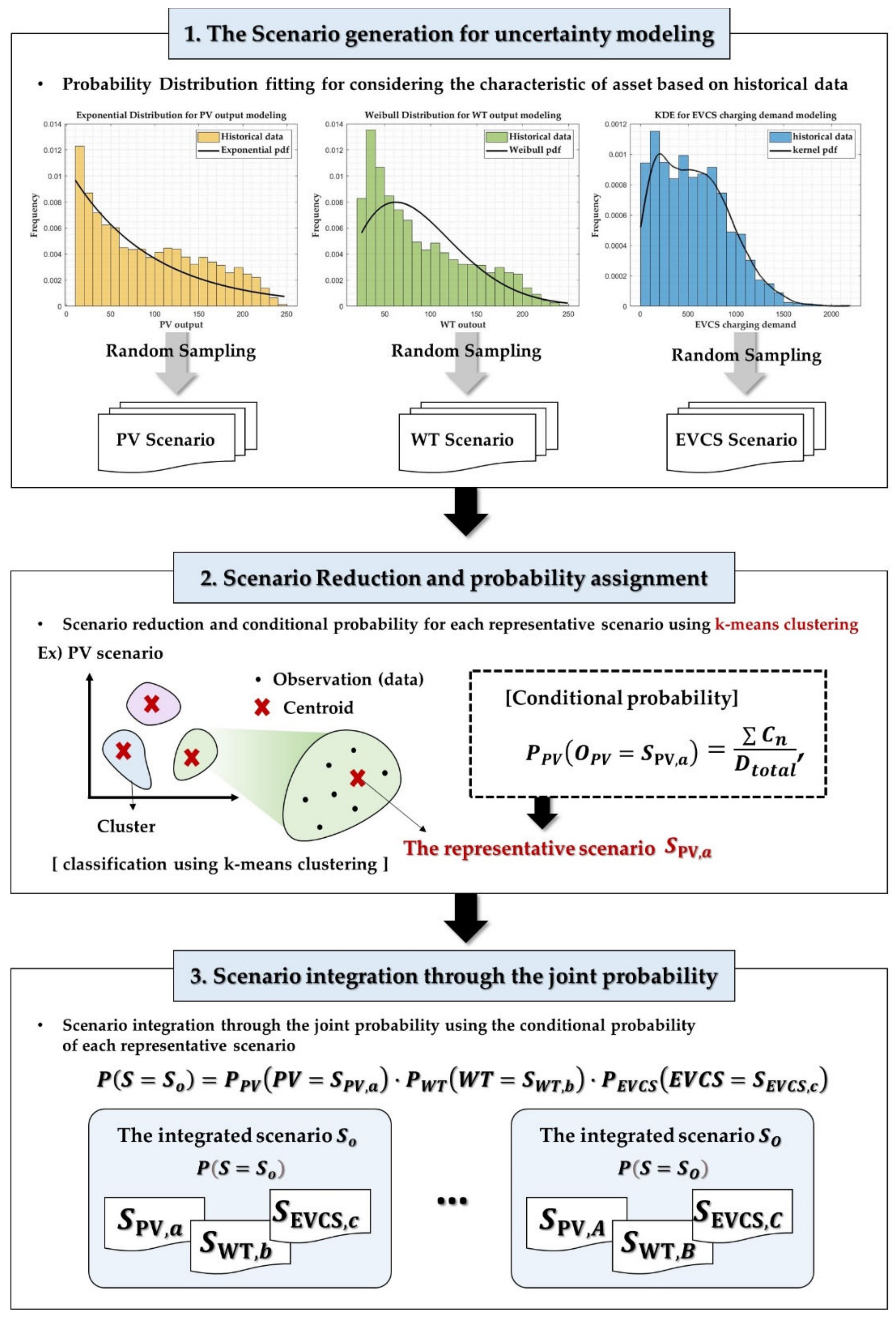
This study aims to appropriately size PV, WT, and EVCS for stable system operation. The following Figure 3 shows the proposed framework for stochastic programming, and

Table 2. The nomenclature for the proposed optimization problem.

Parameter	Meaning
$I_{ij}$	The current of branch $ij$.
$Z_{ij}/R_{ij}$$/X_{ij}$	The impedance/resistance/reactance of branch $ij$.
$V_0$	The nominal voltage.
$V_i$$,V_j$	The $i/j$-th bus voltage.
$V_{1,j}/V_{2,j}$	The auxiliary variables for linearization of objective function.
$S_{ij}/S_{jk}$	The complex power in branch $ij/jk$.
$P_{ij}/P_{jk}$	The active power in branch $ij/jk$.
$Q_{ij}/Q_{jk}$	The reactive power in branch $ij/jk$.
$S_j/P_j/Q_j$	The injected complex/active/reactive power at the $j$-th bus.
$v_i/v_i/l_{jj}$	The auxiliary variables for SOCP relaxation.
$P_{Gi}/Q_{Gi}$	The active/reactive power generated at $j$-th bus.
$\underset{¯}{P_{Gj}},\overline{P_{Gj}}/\underset{¯}{Q_{Gj}},\overline{Q_{Gj}}$	The under and upper bound of $P_{Gi}/Q_{Gi}$.
$P_{Dj}/Q_{Dj}$	The active/reactive power consumed at $j$-th bus.
$\underset{¯}{P_{Dj}}$$,\overline{P_{Dj}}$$/\underset{¯}{Q_{Dj}},\overline{Q_{Dj}}$	The under/upper bound of $P_{Dj}/Q_{Dj}$.
$Ca{p}_{Dj}^{type}$$/Ca{p}_{Gj}^{type}$	The capacity of power-consuming/generating asset.
$\overline{P_{Dj}^{Type}}$$/\overline{P_{Gj}^{Type}}$	The upper bound of active power-consumed/generating asset.
$E{V}_{pen}$	EV penetration rate.
$E{V}_{min}$	The minimum active power of the EVCS.
$P_j^{type}$$/Q_j^{type}$	The active/reactive power of asset at $j$-th bus.
$C_m$	The normalization coefficient of the $m$-th scenario.
$p{f}^{type}$	The power factor of each asset

lists the nomenclature of the proposed optimization problem.

The objective function of the optimization model was to minimize the voltage deviation and line loss using a multi-objective function. This function was formulated as follows:

$$\underset{u}{min}{{\displaystyle \sum }}_{ijϵL}{I}_{ij}^2{R}_{ij}+{{\displaystyle \sum }}_{jϵB}\left|V_o^2-{\left|V_j\right|}^2\right|.$$

(10)

Here, $L$ and $B$ denote the sets of lines and buses in the power system, respectively. $ij$ represents the line connecting the $i$-th and $j$-th bus. $I_{ij}^2$ and $R_{ij}$ represent the current and resistance, respectively, of the line $ij$. $V_0$ is the nominal voltage and $V_j$ is the complex bus voltage at $j$-th bus. That is, $I_{ij}^2{R}_{ij}$ is the line loss of line $ij$ and $\left|V_o^2-{\left|V_j\right|}^2\right|$ is the voltage deviation. $u$ is the set of control variables, which is described in detail in the constraint explanation. However, the objective function is nonlinear owing to the absolute value of the function’s second term. To convexify the objective function, Equation (10) can be rewritten with auxiliary variables as follows:

$$\underset{u}{min}{{\displaystyle \sum }}_{ijϵL}{I}_{ij}^2{R}_{ij}+{{\displaystyle \sum }}_{jϵB}\left(V_{1,j}+V_{2,j}\right).$$

(11)

Here, $V_{1,j}$ and $V_{2,j}$ are auxiliary variables for convexification and positive values. These variables have no physical meaning in the power system, just for linearization. According to the convexification of Equation (11), related constraints were added to ensure equivalence to Equation (10), as follows:

$$V_o^2-{\left|V_j\right|}^2+V_{1,j}-V_{2,j}=0.$$

(12)

$$V_{1,j},V_{2,j}\ge 0.$$

(13)

3.3. Constraints

In general, the AC power flow is nonlinear and non-convex in nature; therefore, DC power flows are extensively applied in practice, and these flows are formulated as linearized power flow equations. DC power flow is convex and makes simulation faster. However, the optimal solution of the DC power flow is incorrect because errors from linearization are inevitable. In this study, the AC power flow was applied to the optimization model and relaxed in the SOCP model with a branch flow model and the remaining AC power flow. Figure 4 presents a summary of the notations used in the branch flow model employed in this study.

$S_{ij}$ and $S_{jk}$ denote the complex powers in branches $ij$ and $jk$, respectively. $P_{ij},P_{jk},Q_{ij}$, and $Q_{jk}$ are the active and reactive powers in each branch, respectively. $S_j$, $P_j$, and $Q_j$ are the injected complex, active, and reactive powers, respectively, of bus $j$. The equations below represent Ohm’s law and the definition of branch power flow, respectively:

$$V_i-V_j=R_{ij}{I}_{ij},$$

(14)

$$S_{ij}=V_i{I}_{ij}^{*}.$$

(15)

where $I_{ij}^{*}$ denotes complex conjugate of $I_{ij}$. Based on the above definition, the power balance at each bus was expressed as follows:

$${{\displaystyle \sum }}_{k\in f_d\left(j\right)}{S}_{jk}-{{\displaystyle \sum }}_{i\in f_u\left(j\right)}(S_{ij}-Z_{ij}{\left|I_{ij}\right|}^2)=S_j.$$

(16)

$f_d\left(j\right)$ and $f_u\left(j\right)$ are the sets of downstream and upstream buses connected to bus $j$. The complex power at the upstream bus is the active power loss attributable to the line impedance. Furthermore, substituting Equation (15) into Equation (14) produces $v_j-v_i=R_{ij}{S}_{ij}^{*}/V_{ij}^{*}$; then, by taking the squared magnitude, we obtain

$${\left|V_j\right|}^2={\left|V_i\right|}^2-2\left(R_{ij}{P}_{ij}+X_{ij}{Q}_{ij}\right)+(R_{ij}^2+X_{ij}){\left|I_{ij}\right|}^2.$$

(17)

However, the equations above are nonconvex because S is a complex number reflecting the angle difference between the real and reactive power, and the bus voltage and branch flow equations include the magnitude squared forms of $V_i, V_j,$ and $I_j$. To convexify these equations, auxiliary variables were introduced as $v_i,v_j,$ and $l_j$, and these notations were substituted into $V_i, V_j,$ and $I_j$. Let $v_i≔{\left|V_i\right|}^2, v_j≔{\left|V_j\right|}^2$, and $l_{ij}≔{\left|I_{ij}\right|}^2$. Thus, these constraints should be separated as real variables and relaxed using auxiliary variables, as follows:

$${\displaystyle \sum }_{k\in f_d\left(j\right)}{P}_{jk}-{\displaystyle \sum }_{i\in f_u\left(j\right)}(P_{ij}-R_{ij}{l}_{ij})=P_j,$$

(18)

$${\displaystyle \sum }_{k\in f_d\left(j\right)}{Q}_{jk}-{\displaystyle \sum }_{i\in f_u\left(j\right)}(Q_{ij}-X_{ij}{l}_{ij})=Q_j,$$

(19)

$$v_j=v_i-2\left(R_{ij}{P}_{ij}+X_{ij}{Q}_{ij}\right)+(R_{ij}^2+X_{ij}^2)l_{ij}.$$

(20)

Here, $P_j$ and $Q_j$ denote the subtraction of the consumption and generation power at bus $j$ and can be expressed as $P_j=P_{Gj}-P_{Dj}$ and $Q_j=Q_{Gj}-Q_{Dj}$, respectively. Indexes $Gj$ and $Dj$ denote the amount of generation and consumption at bus $j$. The constraint-related auxiliary variables $V_1 \mathrm{and} V_2$ were rewritten as follows:

$$V_o^2-v_i+V_1-V_2=0.$$

(21)

Equations (18) and (19) represent the real and reactive power, respectively, separated from the complex power. Then, the constraint due to the auxiliary variable was formulated to represent the relation between the auxiliary variables, real power, and reactive power:

$$l_{ij}=\frac{P_{ij}^2+Q_{ij}^2}{v_i}.$$

(22)

In the power system, the $P_{Gi}, P_{Di}$, $Q_{Gi}, \mathrm{and} Q_{Di}$ of each bus have limited real and reactive powers of generation or demand under conditions of system:

$$\underset{¯}{P_{Gj}}\le P_{Gj}\le \overline{P_{Gj}},\hspace{1em}\hspace{1em}\underset{¯}{Q_{Gj}}\le Q_{Gj}\le \overline{Q_{Gj}},$$

(23)

$$\underset{¯}{P_{Dj}}\le P_{Dj}\le \overline{P_{Dj}},\hspace{1em}\hspace{1em}\underset{¯}{Q_{Dj}}\le Q_{Dj}\le \overline{Q_{Dj}}.$$

(24)

In this study, the power-consuming system assets were the EVCS and generic load, and the power-generating assets were the DG units and substation (slack bus). The $P_{Dj}$ of the power-generating connected bus and the $P_{Gj}$ of the power-consuming connected bus were zero. $P_j$ and $Q_j$ can be classified into five types according to the connected assets: slack, PV, WT, EVCS, and generic load. The capacity of each asset also limits the maximum active power at the connected bus and should always be positive. This can be expressed as

$$0\le Ca{p}_{Dj}^{type}\le \overline{P_{Dj}^{Type}},\hspace{1em}\hspace{1em}0\le Ca{p}_{Gj}^{type}\le \overline{P_{Gj}^{Type}},$$

(25)

where $Ca{p}_{Dj}^{type}$ and $Ca{p}_{Gj}^{type}$ represent the capacities of the power-consuming and power-generating assets, respectively, and $\overline{P_{Dj}^{Type}}$ and $\overline{P_{Gj}^{Type}}$ denote the maximum active power at the asset-connected bus. Furthermore, the EVCS should be able to supply the minimum power for charging, to ensure driver’s convenience; this depends on the EV penetration $E{V}_{pen}$, which is expressed as

$$E{V}_{pen}\times E{V}_{min}\le P_{Dj}^{EVCS}\le \overline{P_{Dj}^{Type}},$$

(26)

where $E{V}_{min}$ denotes the minimum power of the EVCS. The output of the assets should be lower than the capacity and should always have a positive value:

$$P_j=P_j^{type},$$

(27)

$$0\le P_j^{type}\le Ca{p}_j^{type}.$$

(28)

$P_j^{type}$ and $Ca{p}_j^{type}$ are the asset output and capacity, respectively.

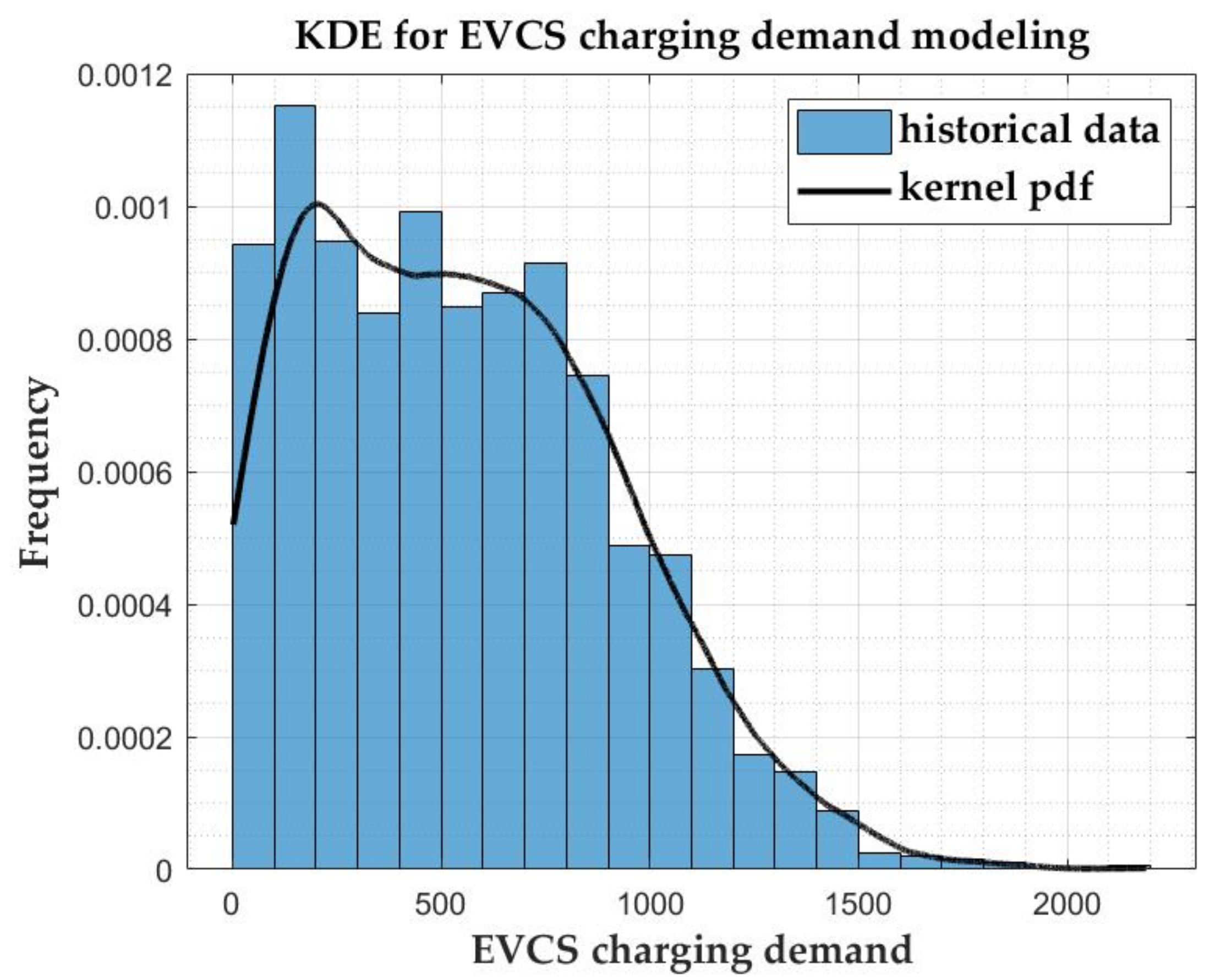
For stochastic programming, the integrated scenario described in Section 2 and the asset output coefficient $C_m$ were applied as follows:

$$P_j^{type}=C_m\times Ca{p}_j^{type}.$$

(29)

Here, $C_m$ denotes the normalization coefficient of the $m_{th}$ scenario. This can be used to reflect the output uncertainty. The reactive power was determined by the active power, because it is assumed that the system assets are operated at a fixed power factor:

$$Q_j=Q_j^{type},$$

(30)

$$Q_j^{type}=P_j^{type}\times \tan {\cos }^{-1}p{f}^{type}.$$

(31)

Here, $p{f}^{type}$ is the power factor of each asset and differs for each one. The line current was limited to the permitted current, to prevent thermal overload:

$$l_{jj}\le {\left|\overline{I_{ij}}\right|}^2.$$

(32)

In addition, the voltage magnitude should be maintained between the allowable lower and upper limits, and the slack bus voltage should be fixed at 1.0 pu:

$${\left|\underset{¯}{V_j}\right|}^2\le v_j\le {\left|\overline{V_j}\right|}^2$$

(33)

However, this problem is still nonconvex, owing to the quadratic equalities in Equation (22). To convexify this problem, conic relaxation was applied to transform the problem into an SOCP. Finally, this constraint was relaxed to inequalities:

$$l_{ij}\ge \frac{P_{ij}^2+Q_{ij}^2}{v_i}.$$

(34)

This inequality constraint is equivalent to the standard form of the SOCP:

$${\Vert \begin{array}{c}2P_{ij}\\ 2Q_{ij}\\ l_{ij}-v_i\end{array}\Vert }_2\le l_{ij}+v_i.$$

(35)

Because the objective function is linear, this optimization problem is a SOCP optimization. In a spanning-tree radial distribution system, the AC power flow relaxation is always exact; the exactness and validation of the SOCP relaxation in AC power flow are proven and comprehensively described in [27,28].

Finally, the proposed optimization problem for the optimal sizing of system assets was reformulated as follows:

$$\underset{u}{min}{{\displaystyle \sum }}_{ijϵL}{l}_{jj}{R}_{ij}+{{\displaystyle \sum }}_{jϵB}(V_{1,j}+V_{2,j}),$$

(36)

$$s.t. \left(12,13\right),\left(18-21\right),\left(23-33\right),\left(35\right).$$

(37)

In the above constraints, the constraints for AC power flow are Equations (18–20), (23), (24), (32), (33) and (35). Equations (12) and (13) are for linearization of the objective function, and other equations are for optimal sizing of each asset.

4. Results and Discussion

In this section, the proposed optimal sizing framework is tested upon a modified IEEE 15-bus radial distribution system.

Table 3. The example for representative scenario of each assets using k-means clustering.

Scenario	PV		WT		EVCS
	Scenario Coefficient	Probability (%)	Scenario Coefficient	Probability (%)	Scenario Coefficient	Probability (%)
1	0.5819	16.83	0.6192	19.65	0.4345	19.18
$2$	0.4278	44.35	0.4594	18.90	0.7838	9.59
$⋮$	$⋮$	$⋮$	$⋮$	$⋮$	$⋮$	$⋮$
Total		1		1		1

shows the representative scenario of each asset using k-means clustering. The normalized data are classified using k-means clustering, and the scenario coefficients are the centroids of each cluster. The k-means clustering is carried out for each asset; therefore, the sum of the probability of occurrence (i.e., the conditional probability) is 1 for each asset.

Table 4. The example of the integrated scenario using the joint probability.

Integrated Scenario	PV	WT	EVCS	Probability (%)
Scenario 1	0.5819	0.6192	0.4345	0.63
Scenario 2	0.5819	0.6192	0.7838	0.32
$⋮$	$⋮$	$⋮$	$⋮$	$⋮$
Scenario 245	0.4943	0.8227	0.5193	0.47
Total				1

represents the example of the integrated scenario using the joint probability. Each integrated scenario includes the scenarios of PV, WT, and EVCS and the probability of each scenario through the joint probability, as shown in Table 4. In this paper, it is assumed that the output of each asset is independent. Therefore, the probability of each integrated scenario is calculated as the product of the probability for representative scenarios.

For this system, case studies are conducted depending on the various optimization functions. Figure 5 illustrates the modified IEEE 15-bus system, and the numbers in Figure 5 represent bus number.

Table 5. System parameters.

Parameter	Value	Parameter	Value
$E{V}_{min}$ (kW)	350	$V_0$ (kV)	12
$Ca{p}^{max}$ (MW)	12	$p{f}^{EVCS}$	0.99 lag
$V_{min}$ (pu)	0.95	$p{f}^{PV}$	0.99 lag
$V_{max}$ (pu)	1.05	$p{f}^{WT}$	0.95 lag

lists the system parameters, and the parameter and decision variables in the proposed optimization are applied as per unit. The DG units and EVCS were in Bus 7, 8, and 11 and Bus 13, respectively.

A case study analysis was carried out for different objective functions, as follows:

• Case 1 ($C_A$ = 1, $C_B$ = 0): Line loss minimization (active power loss);
• Case 2 ($C_A$ = 0, $C_B$ = 1): Voltage deviation minimization;
• Case 3 ($C_A$ = 1, $C_B$ = 1): Line loss and voltage deviation minimization (multi-objective function).

To implement the optimization of various objective functions, the objective function was rewritten as

$$\underset{u}{min}{C}_A{{\displaystyle \sum }}_{ij=1}^L{I}_{ij}^2{R}_{ij}+C_B{{\displaystyle \sum }}_{j=1}^B(V_{1,j}-V_{2,j}).$$

(38)

The simulation results are presented in

Table 6. Results of the optimal sizing of system assets.

Asset	Case 1	Case 2	Case 3
EVCS1 (kVA)	685.7	685.7	685.7
EVCS2 (kVA)	685.8	3051.5	3048.6
PV (kVA)	7971.9	7858.8	10,377.4
WT (kVA)	3921.6	$0$	3743.1
Active power loss (Line loss) (kW)	608	3737.1	706.7
Voltage deviation (pu)	0.4905	0.1343	0.3393

. Comparing Cases 1 and 2, it can be seen that the active power loss in Case 2 decreased substantially (by 83.7% in Case 1) because the objective function minimizes the line loss of the test system. In contrast, the voltage deviation in Case 2 was ~27.3% less than that in Case 1, because the objective function of Case 2 was to minimize the voltage deviation. The voltage deviation in Table 6 was obtained as follows:

$$Voltage deviation={\displaystyle \sum }_{j\in B}\left|V_o-V_j\right|.$$

(39)

In Case 1, the size of EVCS2 was smaller than that of the other cases because EVCS2 was located at the end of the system, and the line loss due to line impedance was large. The size of the WT was zero. From the perspective of minimizing the voltage, DG units can cause overvoltage at the DG-connected bus. EVCS1 was located close to the substation, and the capacity of EVCS1 was smaller than that of EVCS1. Hence, the size of WT was zero, to minimize the voltage deviation. It can be noted that the results (i.e., the capacities of asset, loss, and voltage deviation) in Cases 1 and 2 were strongly determined by the objective to be minimized, which is not appropriate. Hence, a multi-objective function was applied in this study (see Case 3). The voltage deviation and line loss were lower than in Cases 1 and 2, respectively. From the cases, the impact of the auxiliary variables $V_{1,j}$ and $V_{2,j}$ for convexifying the objective function can be analyzed. Case 2, which minimizes only voltage deviation, shows the smallest voltage deviation. Additionally, when comparing Cases 1 and 3, the effect of the auxiliary variables can be verified by reducing the voltage deviation in Case 3 where both loss and voltage deviation are minimized compared to Case 1 where only power loss is minimized.

Figure 6, Figure 7 and Figure 8 show the bus voltage of each scenario in the case studies. The bus voltages at the asset-connected bus are listed in detail in

Table 7. Bus voltage in each case.

Bus	Case 1	Case 2	Case 3
7 (EVCS1)	1.0241	1.0000	1.0207
8 (WT)	1.0500	1.0037	1.0457
11 (PV)	1.0500	1.0500	1.0500
13 (EVCS2)	1.0399	1.0000	1.0000

. The objective function that minimizes the voltage deviation was not included in Case 1, and the bus voltage in Figure 6 shows that the voltage deviation exceeded that in other cases. It can be observed in Figure 7 that the bus voltage of Case 2 (in which only the voltage deviation was minimized) exhibited the smallest voltage deviation. In Figure 7, compared to other cases, the voltage at Bus 8 (connected to the WT) was closest to 1.0 pu, because the wind power generation was zero and therefore the voltage did not increase. A voltage greater than 1.0 pu appeared on the DG-connected or adjacent buses. As shown in Table 7., the voltages on the DG-connected bus and EVCS-connected bus exceeded 1.0 pu, because the EVCSs were located close to the DG units.

It should be noted in Figure 6, Figure 7 and Figure 8 that the voltage did not depend on the scenario. In the proposed optimization model, the capacity of an asset depends on the scenario that minimizes voltage deviation and line loss. Figure 9, Figure 10 and Figure 11 show the change in capacity with respect to the scenario. In the case of case 1, it is calculated that charging stations 1 and 2 have almost the same capacity, and WT is the most calculated compared to other cases. In Case 2, it can be observed that the capacity of WT is calculated as 0 in all scenarios, as shown in Table 6. The capacity of EVCS 2 is calculated to be larger in all Cases 2 and 3 because EVCS is adjacent to a bus connected with a PV with a large output. It can be confirmed that, in Case 3, the capacity of WT is calculated to be larger than in Case 2, and that the capacity of EVCS2 is calculated to be larger than in Case 1.

Table 8. Comparison of cases with/without k-means clustering.

Asset	With k-Means Clustering		Without k-Means Clustering
	Capacity (pu)	Computation Time (s)	Capacity (pu)	Computation Time (s)
EVCS1 (kVA)	685.7	5.37	5378.7	208.40
EVCS2 (kVA)	3048.6		236,905
PV (kVA)	10,377.4		265,649.4
WT (kVA)	3743.1		11,619.9

represents the comparison of with/without k-means clustering. Compared to the case where scenario reduction using the k-means clustering is applied, it can be found that the capacity is extremely oversized when it is not applied. This is because there are many scenarios close to zero, so the capacity is calculated excessively. In addition, because the number of scenarios is large, the operation time is also larger than the case where the k-means clustering is applied, about 208 s, and it can be verified that the scenario reduction through the application of the k-means clustering is effective in the optimal sizing framework of system asset.

5. Conclusions

A new method for optimally sizing PV, WT, and EVCS was proposed to minimize voltage deviation and line loss. The proposed method is formulated as a stochastic SOCP model to consider the uncertainties of the system assets and applied AC power flow. To consider the uncertainties, the probability distribution was fitted according to the output characteristics of the PV, WT, and EVCS; then, integrated scenarios were generated using k-means clustering. Finally, these integrated scenarios were applied to the stochastic SOCP optimization model.

To verify the effectiveness of the proposed optimization model, case studies involving various objective functions were conducted, and these cases were compared with each other. When a single objective function was applied, the capacity of the asset and system value (e.g., line loss and voltage deviation) was robustly determined, whereas the multi-objective function model determined the control variables (e.g., line loss, voltage deviation, and capacity). These results were confirmed through numerical experiments and analyses of multiple dimensions.

The proposed method can solve ADN planning problems by considering these uncertainties. Furthermore, the power system was considered by employing an AC power flow in the model. The optimal sizing of the DG units and EVCS was properly determined in the distribution planning step.

However, the EV charging demand was simplified by modeling the charging demand from the EVCS rather than the driver’s perspective. The generated scenarios are not time-variant but a snapshot for a certain time. Therefore, we will model the driver’s behavior characteristics in future work and generate a time-variant scenario (i.e., profile scenario for PV, WT, and EVCS). This model will be applied in charging demand modeling for ADN planning; furthermore, the joint optimal sizing and siting model of DGs and EVCSs will be extended to achieve greater practical value. This work will help resolve the problems of uncertainty in ADN planning and thereby offer breakthroughs in the design of economical and reliable energy systems for the future.

References

1. Shahab, B.; Amini, M.H. A decentralized trading algorithm for an electricity market with generation uncertainty. Appl. Energy 2018, 218, 520–532. [Google Scholar]
2. Luo, L.; Gu, W.; Wu, Z.; Zhou, S. Joint planning of distributed generation and electric vehicle charging stations considering real-time charging navigation. Appl. Energy 2019, 242, 1274–1284. [Google Scholar] [CrossRef]
3. Wang, S.; Dong, Z.Y.; Chen, C.; Fan, H.; Luo, F. Expansion Planning of Active Distribution Networks with Multiple Distributed Energy Resources and EV Sharing System. IEEE Trans. Smart Grid 2020, 11, 602–611. [Google Scholar] [CrossRef]
4. Stott, B.; Alsac, O. Fast Decoupled Load Flow. IEEE Trans. Power Appar. Syst. 1974, PAS-93, 859–869. [Google Scholar] [CrossRef]
5. Alsac, O.; Bright, J.; Prais, M.; Stott, B. Further developments in LP-based optimal power flow. IEEE Trans. Power Syst. 1990, 5, 697–711. [Google Scholar] [CrossRef]
6. Purchala, K.; Meeus, L.; Van Dommelen, D.; Belmans, R. Usefulness of DC power flow for active power flow analysis. In Proceedings of the IEEE Power Engineering Society General Meeting, San Francisco, CA, USA, 16 June 2005; pp. 454–459. [Google Scholar]
7. Stott, B.; Jardim, J.; Alsac, O. DC Power Flow Revisited. IEEE Trans. Power Syst. 2009, 24, 1290–1300. [Google Scholar] [CrossRef]
8. Javadi, M.S.; Gouveia, C.S.; Carvalho, L.M.; Silva, R. Optimal Power Flow Solution for Distribution Networks using Quadratically Constrained Programming and McCormick Relaxation Technique. In Proceedings of the 2021 IEEE International Conference on Environment and Electrical Engineering and 2021 IEEE Industrial and Commercial Power Systems Europe (EEEIC/I&CPS Europe), Bari, Italy, 7–10 September 2021; pp. 1–6. [Google Scholar]
9. Mamun, K.A.; Islam, F.R.; Haque, R.; Chand, A.A.; Prasad, K.A.; Goundar, K.K.; Prakash, K.; Maharaj, S. Systematic Modeling and Analysis of On-Board Vehicle Integrated Novel Hybrid Renewable Energy System with Storage for Electric Vehicles. Sustainability 2022, 14, 2538. [Google Scholar] [CrossRef]
10. Kandil, S.M.; Farag, H.E.; Shaaban, M.; El-Sharafy, M.Z. A combined resource allocation framework for PEVs charging stations, renewable energy resources and distributed energy storage systems. Energy 2018, 143, 961–972. [Google Scholar] [CrossRef]
11. Ahmadian, A.; Aliakbar-Golkar, M. Fuzzy load modeling of plug-in electric vehicles for optimal storage and DG planning in active distribution network. IEEE Trans. Veh. Technol. 2016, 66, 3622–3631. [Google Scholar] [CrossRef]
12. De Quevedo, P.M.; Muñoz-Delgado, G.; Contreras, J. Impact of electric vehicles on the expansion planning of distribution systems considering renewable energy, storage, and charging stations. IEEE Trans. Smart Grid 2017, 10, 794–804. [Google Scholar] [CrossRef]
13. Zheng, Y.; Song, Y.; Hill, D.J.; Meng, K. Online Distributed MPC-Based Optimal Scheduling for EV Charging Stations in Distribution Systems. IEEE Trans. Ind. Inform. 2019, 15, 638–649. [Google Scholar] [CrossRef]
14. Erdinc, O.; Tascikaraoglu, A.; Paterakis, N.G.; Dursun, I.; Sinim, M.C.; Catalao, J.P.S. Comprehensive Optimization Model for Sizing and Siting of DG Units, EV Charging Stations, and Energy Storage Systems. IEEE Trans. Smart Grid 2018, 9, 3871–3882. [Google Scholar] [CrossRef]
15. Amini, M.H.; Moghaddam, M.P.; Karabasoglu, O. Simultaneous allocation of electric vehicles’ parking lots and distributed renewable resources in smart power distribution networks. Sustain. Cities Soc. 2017, 28, 332–342. [Google Scholar] [CrossRef]
16. Wang, G.; Xu, Z.; Wen, F.; Wong, K.P. Traffic-Constrained Multiobjective Planning of Electric-Vehicle Charging Stations. IEEE Trans. Power Deliv. 2013, 28, 2363–2372. [Google Scholar] [CrossRef]
17. Liu, Z.; Wen, F.; Ledwich, G. Optimal siting and sizing of distributed generators in distribution systems considering uncertainties. IEEE Trans. Power Deliv. 2011, 26, 2541–2551. [Google Scholar] [CrossRef]
18. Amer, A.; Azab, A.; Azzouz, M.A.; Awad, A.S.A. A Stochastic Program for Siting and Sizing Fast Charging Stations and Small Wind Turbines in Urban Areas. IEEE Trans. Sustain. Energy 2021, 12, 1217–1228. [Google Scholar] [CrossRef]
19. Fan, V.H.; Dong, Z.; Meng, K. Integrated distribution expansion planning considering stochastic renewable energy resources and electric vehicles. Appl. Energy 2020, 278, 115720. [Google Scholar] [CrossRef]
20. Thangaraju, I. Optimal allocation of distributed generation and electric vehicle charging stations-based SPOA2B approach. Int. J. Intell. Syst. 2022, 37, 2061–2088. [Google Scholar] [CrossRef]
21. Muñoz-Delgado, G.; Contreras, J.; Arroyo, J.M. Joint expansion planning of distributed generation and distribution networks. IEEE Trans. Power Syst. 2014, 30, 2579–2590. [Google Scholar] [CrossRef]
22. Yuwei, C.; Xiang, J.; Li, Y. SOCP relaxations of optimal power flow problem considering current margins in radial networks. Energies 2018, 11, 3164. [Google Scholar]
23. Zhang, H.; Moura, S.J.; Yonghua, S.; Qi, W.; Song, Y. A Second-Order Cone Programming Model for Planning PEV Fast-Charging Stations. IEEE Trans. Power Syst. 2018, 33, 2763–2777. [Google Scholar] [CrossRef] [Green Version]
24. Farivar, M.; Low, S.H. Branch flow model: Relaxations and convexification—Part I. IEEE Trans. Power Syst. 2013, 28, 2554–2564. [Google Scholar] [CrossRef]
25. Luo, L.; Gu, W.; Zhang, X.-P.; Cao, G.; Wang, W.; Zhu, G.; You, D.; Wu, Z. Optimal siting and sizing of distributed generation in distribution systems with PV solar farm utilized as STATCOM (PV-STATCOM). Appl. Energy 2018, 210, 1092–1100. [Google Scholar] [CrossRef]
26. Feijoo, A.E.; Cidras, J.; Dornelas, J.L.C. Wind speed simulation in wind farms for steady-state security assessment of electrical power systems. IEEE Trans. Energy Convers. 1999, 14, 1582–1588. [Google Scholar] [CrossRef]
27. Sheather, S.J.; Jones, M.C. A reliable data-based bandwidth selection method for kernel density estimation. J. R. Stat. Soc. Ser. B Methodol. 1991, 53, 683–690. [Google Scholar] [CrossRef]
28. NEOS. Stochastic Linear Programming. Available online: https://neos-guide.org/content/stochastic-linear-programming (accessed on 16 February 2022).
Figure 1. The framework for the proposed scenario generation method.
Sustainability 14 04964 g001
Figure 2. Histogram of charging demand data and kernel density estimation-based PDF.
Sustainability 14 04964 g002
Figure 3. The flowchart for the proposed stochastic SOCP optimization.
Sustainability 14 04964 g003
Figure 4. The 3-bus system for method demonstration.
Sustainability 14 04964 g004
Figure 5. Modified IEEE 15-bus system.
Sustainability 14 04964 g005
Figure 6. Bus voltage for Case 1.
Sustainability 14 04964 g006
Figure 7. Bus voltage for Case 2.
Sustainability 14 04964 g007
Figure 8. Bus voltage for Case 3.
Sustainability 14 04964 g008
Figure 9. Capacity with respect to scenario for Case 1.
Sustainability 14 04964 g009
Figure 10. Capacity with respect to scenario for Case 2.
Sustainability 14 04964 g010
Figure 11. Capacity with respect to scenario for Case 3.
Sustainability 14 04964 g011