The State of the Art and New Insight into Combined Finite–Discrete Element Modelling of the Entire Rock Slope Failure Process

Abstract

The stability of rock slopes is of significance, as even the slightest slope failure can result in damage to infrastructure and catastrophes for human beings. Thus, this article focuses on the review of the current techniques available for rock slope stability analysis. The rock slope stability techniques can be classified as conventional methods and numerical methods. The advantages and limitations of the conventional method are briefly reviewed. The numerical methods mainly included three types, i.e., continuum methods, discontinuum methods, and the combined/hybrid continuum–discontinuum methods. This article pays more attention to the last type. The combined/hybrid finite–discrete element method (FDEM), which might be the most widely used continuum–discontinuum method, is introduced and we illustrated its abilities in modelling the entire rock slope failure process. The fundamental principles of FDEM, i.e., the contact interaction of the discrete bodies and the transition from continuum to discontinuum, are introduced in detail. The abilities of the FDEM in modelling the rock slope failure process are calibrated by modelling the entire typical rock slope failure process. Then, the application of the FDEM in the analysis of slope stability is introduced and discussed. Finally, the authors give insight into the GPGUP-parallelized FDEM modelling of the high rock slope failure process by the implementation of the strength reduction method (SRM). It is concluded that the FDEM can effectively model the entire rock slope failure process, even without the implantation of any slope modes, and the GPGUP-parallelized FDEM is a promising tool in the study and application of rock slope stabilities.

1. Introduction

The fast development of modern society results in a variety of geotechnical activities, some of which require the excavation of rock cuts. Those actives, e.g., embayment, open-pit mining, and highway and urban contraction, can form many slopes. Figure 1 gives two typical rock slope examples. Figure 1a illustrates a rock slope with an angle of about 60° for the surface, which is reinforced by tensioned anchors. Figure 1b is a typical rock slope formed due to mining excavation in the Palabora open pit. The slope is 830 m in depth with an overall slope angle of 45–50°. There are also natural rock slopes in addition to the man-made slopes. For instance, the mountains or valleys are generally steep or falter slopes. As highways or railways might be built along valleys, the stability of the slopes, whether man-made or natural, are of significance in terms of protecting the surroundings and avoiding casualties.

The slope stability is always seen as critical, since even the tiniest slope failure may be costly in terms of monetary damage and human lives. It is essential to understand the geological, geomorphological, and hydrogeological characterization of a slope before the reconstruction of any structure. More importantly, a comprehensive understanding of the impacts of the external factors, e.g., external loading, seismicity, and groundwater, is crucial for preventing and controlling slope instabilities. In addition, the rock characteristics of the slope, e.g., faults, folds, and discontinuities, are significant factors influencing the stabilities of the rock slopes. The stability analysis of the rock slope is always associated with the factor of safety, which is the most well-known performance indicator in slope stability. The factor of the safety of the rock slope is a ratio of the average shear strength of a specific slip face to the average applied shear stress. If the ratio, i.e., the factor of the safety $\mathrm{F}=1$, it represents the “critical equilibrium” or “limiting equilibrium”, and this implies that a slope is on the verge of collapse or sliding, or complete failure. In this scenario, the rock slide is imminent along a certain slip surface. If the factor of the safety $\mathrm{F}>1$, the slope is stable and it is not on the verge of sliding. If the factor of the safety $\mathrm{F}<1$, it represents instability, and in this case, the slope design cannot be constructed.

In general, the rock slope has four categories in terms of failure types, i.e., plane failures, wedge failures, toppling failures, and circular failures. Figure 2a illustrates a general sketch of a plane failure (left part) and the plane failure of a rock slope in a mountain (right part). As illustrated in Figure 2a, for a plane failure, there is a structural discontinuity plane where sliding occurs. The angle of the discontinuity plane is smaller than the slope-face angle and it is greater than the fraction angle of the discontinuity surface [2]. Figure 2b illustrates the edge failure of the rock slope. It involves two discontinuities inclined out of the slope face and a rock mass, such as a wedge on them. During the edge failure, the wedge-like rock mass is generated and slides along the two crossing discontinuities that both drop out of the cut slope at an oblique angle to the curt face. Figure 2c shows the toppling failures of rock slopes. Toppling failures are most prevalent in rock masses that have been broken into a series of slabs or columns by a sequence of fractures that run roughly parallel to the slope face and dip sharply into it. Figure 2d illustrates the circular failure of the rock slope, which is named by the failure type—like the arc of a circle. It often occurs in solid mass with large grain sizes. Thus, for the circular failure of the rock slope, the rock mass is generally fragmented and the failure is not predominately controlled by a discontinuity (e.g., plane failure) or two intercrossing discontinuities (e.g., wedge failure).

The rock slope stability analysis is essential for many engineering projects, e.g., road cuts and open-pit mining. The main purposes of the rock slope stability analysis are to determine the stability of the rock slope, to investigate the different support options, and to optimize the slope in terms of reliability. There are many techniques available for performing the analyses, which can be in general classified into the conventional methods and numerical methods. The conventional methods include limit equilibrium techniques and the kinematic method. Limit equilibrium techniques are popular methods for the analysis of the plane or the toppling failure of the rock slope. This technique can provide a factor of safety or it can provide shear strength parameters for a rock slope. There are also lots of computer programs used for slope instability analysis, which are made based on the limit equilibrium concept [5]. The limit equilibrium approach has traditionally been used to test the stability of rock slopes, which are confined to the analysis of planar or wedge instabilities, while other complicated failure kinematics, such as toppling, are often not addressed by these methodologies.

The numerical methods are significant tools utilized during the slope design stage. As for the numerical techniques, there are mainly two categories, i.e., the continuum method and the discontinuum method. The representative continuum methods for modelling the rock slopes are the finite element method [6], failure-process analysis method (RFPA) [7], numerical manifold method (NMM) [8], and finite difference method (FDM) [9]. Jin, Yin and Yuan (2020) used the smooth-particle finite element method to simulate the rock slope failure process [6]. The smooth-particle finite element method is an updated Lagrangian approach with frequent re-meshing by the Delaunay triangulation method [6]. To employ continuum modelling, the rock mass in the slope is considered as a continuum material. In addition, the finite element method is widely used to study the failure mechanisms of the unsupported conical slope by the implementation of various rock failure models and criteria [10,11,12,13,14], e.g., the anisotropic undrained shear (AUS) model [11] and the Hoek–Brown failure criterion. However, for a real rock slope, there are unavoidable pre-existing planes of weaknesses, e.g., schistosity, joint sets, and faults. Those weaknesses in the rock slope might be the key issues that result in the instability of the rock slope. The continuum technique has limits in explicitly simulating complicated discontinuities, progressive failure, substantial deformation, and complex rock movement during the whole failure process due to the continuum assumptions [15]. There is also a variety of discontinuum methods applied for the simulation of the rock slope failure process. The distinct element method (DEM) [16] might be the most widely used discontinuum method. Jiang and Murakami (2012) employed the distinct-element method to model the full-process slope failure. The particle flow code (PFC) [7] and the discontinuous deformation analysis method (DDA) [17] are widely used to model the slope failure process.

The rock slope failure process is extremely complicated, it involves crack initiation propagation, and coalescence, and rock-bodies movement, rotation, and fragmentation. Neither the continuum method nor the discontinuum method can solve these problems [18]. Thus, a more robust numerical method, taking the advantages of both the continuum method and discontinuum method, is needed to reproduce the full failure process. The continuum–discontinuum method might be the most suitable technique to model the entire rock failure process, as it combines the advantage of the continuum-based methods and the discontinuum-based methods. Many researchers have focused their studies on the continuum–discontinuum modelling of the rock slope failure process [19,20,21,22,23]. Thus, this research reviews the rock slope sliding modelling using the continuum–discontinuum method. As the hybrid finite–discrete element method (FDEM) is one of the most popular approaches to modelling the rock fracture process, and

Table 1. Summary of FDEM modelling of the rock slope failure process.

Numerical Code	Modelled Results	Reference
Y-Slope	Y-Slope considers the tensile and shear failure. The failure is caused by gravity. By decreasing the strength parameters, the cracks initiate from the toe of the slope and propagate further into the slope. Finally, the cracks form a discontinuity surface. The crack initiation, propagation, colliding, fragmentation, and piling are modelled.	[19]
FDEM realized using ABAQUS/Explicit	The FDEM framework is implemented in the ABAQUS/Explicit. The cohesive zone model (CZM) is employed to model the fracture occurring along the bulk elements boundary. The gravity increase method is implanted in the ABAQUS/Explicit-based FDEM program to model the slope failure process. The failure processes of the laboratory-scale slope with various joint inclination surfaces are modelled.	[20]
Y-Geo based on Munjiza’s Y-code	Y-Geo is used to model the evaluation of a rock slide that occurred in Italy in 1997. The modelled results in terms of the runout profiles and evaluation of the slopes agree well with the site observation.	[21]
ELFEN	A modified Mohr–Coulomb elastoplastic model is implemented in ELFEN to model the material softening, and deal with both the tension and shear states. Then, the ELFEN was employed to model the 1991 Randa rockslide. Due to strength degradation, the rock mass breaks into blocks and are modelled using ELFEN.	[23]
Y-2D with Y-GUI	The failure process of the rock avalanche is modelled. The weak interface in the slope was firstly produced, then, the rock avalanche was initiated. A large volume of rock mass started to move, which further fragmented. During the process, the blocks were progressively broken into smaller fragments.	[22]

lists the representative study on the FDEM modelling of rock slope failure processes, this research introduced the main principles of the hybrid finite–discrete element method. In addition, the calibrated applications of the hybrid finite–discrete element method are introduced and explained in detail to demonstrate the validity and capability of the hybrid finite–discrete element method in modelling the entire rock slope failure process.

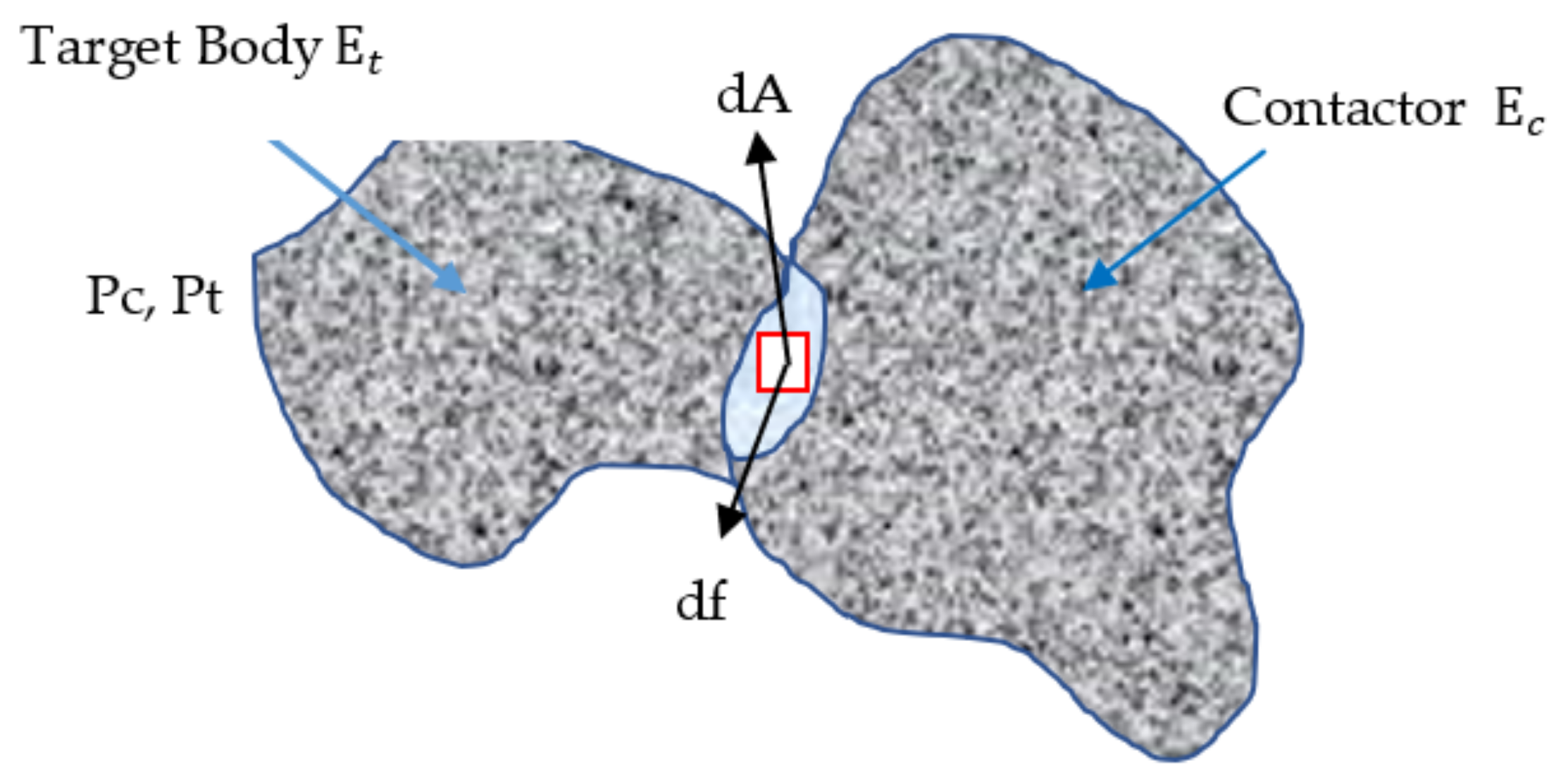
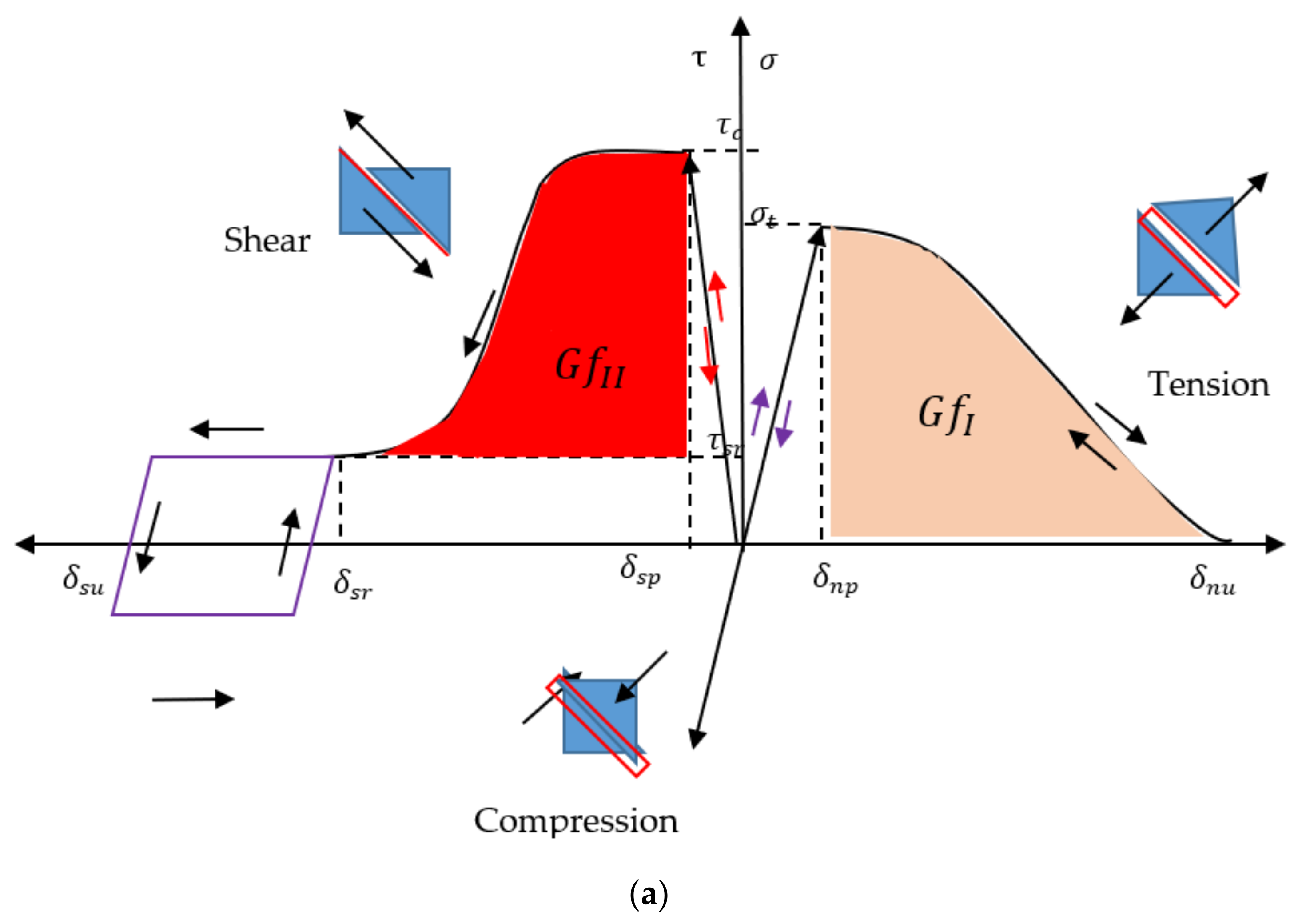
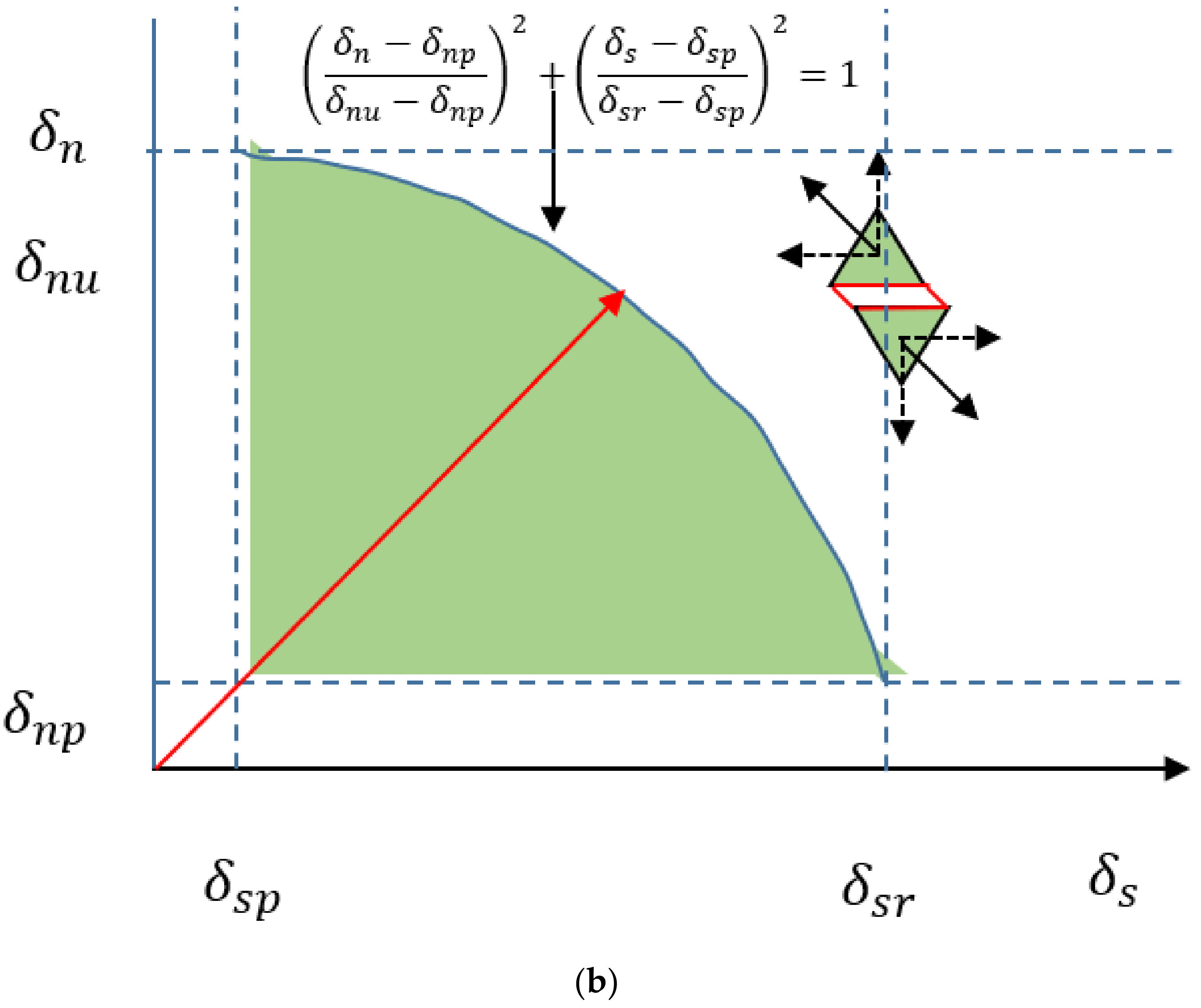
2. Combined Finite–Discrete Element Method

The continuum–discontinuum method (CDM) is a promising tool for the study of the rock fracture and fragmentation process under static or dynamic loading conditions, e.g., blasting [24,25,26,27,28,29,30]. It has been successfully applied in many geotechnical engineering problems associated with the transition from continuum to discontinuum through fracture and fragmentation over the last two decades [31,32,33,34]. Compared with the continuum method or discontinuum method, the CDM can not only model the rock damage, fracture initiation, coalescence, and propagation as most of the continuum-based methods do, but it also can model the interaction of the fracture rocks and even the muck-pilling of the rock fragments during a rock blasting process [30]. Many CDM methods have been proposed for overcoming the shortcomings of the continuum-based method or discontinuum method in simulating the entire rock fracture process, e.g., the combination of the boundary element method with the finite element method (BEM/FEM), the combination of the discrete element method with the finite element method (DEM/FEM), and the combination of the discrete element method with the boundary element method (DEM/BEM) [35].

The hybrid/combined finite element method (FDEM) might be the most widely used continuum–discontinuum method. Based on the FDEM, many tools are developed for modelling the entire rock fracture process, e.g., Y-2D [36], Y-GUI [37], Y-GEO [30], Y-Slope [19], Y2D/3D IDE [30], and the commercial software ELFEN [38,39]. Y-slope models the crack initiation, propagation, colliding, fragmentation and pilling process during the rock slope failure process [19]. Y2D/3D IDE has been implemented to model the entire fracture, fragmentation, and muck-pilling process induced by the blast [30], and has also been used to study the excavation damaged zone (EDZ) induced by blasting in deep tunnels [29]. Y-GUI is a graphical user interface developed for Y2D, as Y2D setting up Y2D modes is a time-consuming and error-prone process [22]. The GUI is developed to setup Y-2D modes graphically and minimize the possibility of erroneous input files [22]. Y2D has modelled the slope failure process where rock avalanches occur [22].

As the FDEM has been used in many geotechnical problems, the fundamental principles and FDEM applications have been introduced in detail. For a FDEM mode, it can have one discrete body or many discrete bodies. As illustrated in Figure 3, the discrete body is meshed by three-node finite elements (Figure 3a), and the four-node joint elements (Figure 3b) are embedded among the finite elements. The damage and the deformity of the rock mass are modelled using the three-node finite element, while the fracture initiation and propagation are simulated by the distortion of the four-node joint elements depending on the calculated strains on the finite element of a discrete.

Sun et al. (2022) [19] gave the rock mass with fracture and its equivalent FDEM model meshed by three-node finite element and four-node joint elements, as illustrated in Figure 4. The rock model is meshed using finite elements and the cracks are modelled using the broken joint elements, i.e., crack elements. The stress and strain of the individual body are described using the continuum law. The fracture of the rock, i.e., the transition from continuum to discontinuum, is modelled by the breakage of the joint element among the three-node finite elements. The motion of each node of the discrete body is updated using Newton’s second law (Equation (1) [40]).

$$M\frac{{\partial }^{2}X}{\partial t^2}+C\frac{\partial X}{\partial t}=F$$

(1)

where M is the mass of the discrete body while C is the damping diagonal matrices, X is the nodal displacement and F is the node force vector.

Figure 3. FDEM modelling rock fracture modes [19,25,27,28,41]. (a) FDEM model assembled with three-node and four-node elements (from reference [41]); (b) tensile failure (from reference [28]); (c) shear failure (from reference [27]); (d) mixed tensile–shear failure (from reference [25]).

Figure 3. FDEM modelling rock fracture modes [19,25,27,28,41]. (a) FDEM model assembled with three-node and four-node elements (from reference [41]); (b) tensile failure (from reference [28]); (c) shear failure (from reference [27]); (d) mixed tensile–shear failure (from reference [25]).

Contact detections of the discrete elements or discrete bodies are essential for the FDEM, as there might be thousands or even millions of discrete elements or discrete bodies. Thus, many algorithms for automatic contact detection are proposed [36,42], e.g., the no-binary search, buffer zone, binary tree, and alternating digital tree. After the coupled discrete elements or discrete bodies are detected, the contact forces between the coupled discrete elements or bodies are calculated.

Most of the FDEMs use the penalty method to calculate the contact forces in the tangential and normal directions [26,36]. As illustrated in Figure 5, the two bodies are called the target and contactor, respectively. The penetration of the contactor into the target causes contact force. An infinitesimal contact force due to the penetration can be calculated using Equation (2) [36], while the total contact force due can be calculated using Equation (3) [36].

$$\mathrm{df}=\left[grad{\phi }_c\left(P_c\right)-grad{\phi }_t\left(P_t\right)\right]dA$$

(2)

$${\mathrm{f}}_{\mathrm{c}}={{\displaystyle \int }}_{S=E_{t\cap E_c}}^{ }\left(grad{\phi }_c\left(P_c\right)-grad{\phi }_t\left(P_t\right)\right)dA$$

(3)

where $\mathrm{df}$ is the infinitesimal overlap $dA$ force and the ${\phi }_c$ and ${\phi }_t$ are potential functions.

During the contact interaction, the discrete element or bodies are deformable and the joint elements can be distorted to perform the continuum of the rock mass. The distortion in the vertical and normal direction will finally result in the shear and tensile failure, which perform the transition of the intact rock from continuum to discontinuum through the rock fracture and fragmentation. Bonding stress is induced during the distortion or the separation of the joint elements. Figure 6 gives the relationship between the bonding stresses with the separation of the joint elements in the normal direction (Figure 6a, right), and the vertical direction (Figure 6a, left). The bonding stress in the normal direction can be obtained according to Equation (4) [43]:

$${\sigma }_n=\left\{\begin{array}{ccc}\left[2·\frac{{\delta }_n}{{\delta }_{np}}-{\left(\frac{{\delta }_n}{{\delta }_{np}}\right)}^2\right]·{\sigma }_t& if& 0\le {\delta }_n\le {\delta }_{np}\\ f\left(D\right)·{\sigma }_t& if& {\delta }_{np}\le {\delta }_n\le {\delta }_{nu}\\ 0& if& {\delta }_n\ge {\delta }_{nu}\end{array}\right.$$

(4)

The tensile fracture or the Mode-I fracture process is governed by the Mode-I fracture energy release, and the value can be calculated as follows (Equation (5) [43]).

$${\mathrm{G}}_{fI}=\underset{ {\delta }_{np}}{\overset{ {\delta }_{nu}}{{\displaystyle \int }}}{\sigma }_n\left( {\delta }_n\right)d{\delta }_n$$

(5)

where the ${\mathrm{G}}_{fI}$ is the Mode-I fracture energy release rate.

For the shear fracture or the Mode-II fracture process, the sliding of the adjacent finite element and the shear stress relationship is illustrated in the right part of Figure 6a. The shear stress $\mathsf{\tau }$ increases with the increase of the sliding ${\delta }_s$ and the shear strength corresponds to the sliding displacement of ${\delta }_{sp}$, which indicates the shear fracture occurs. After that, the boding stress in the tangential direction or the shear stress decreases. As it decreases to a residual stress ${\delta }_{sr}$ according to a mechanical damage model, the shear fracture finishes. The bonding stress in the tangential direction can be expressed as Equation (6) [43] according to the sliding displacement of the adjacent finite elements.

$$\tau =\left\{\begin{array}{ccc}2·\frac{{\delta }_s}{{\delta }_{sp}}·{\sigma }_c& if& 0\le {\delta }_s\le {\delta }_{sp}\\ g\left(D\right)& if& {\delta }_{sp}\le {\delta }_s\le {\delta }_{sr} \\ {\sigma }_n·tan\left({\varnothing }_f\right)& if& {\delta }_s\ge {\delta }_{sr}\end{array}\right.$$

(6)

where D is the damage variable and $g\left(D\right)$ is the function of the damage [44], and ${\varnothing }_f$ is the joint residual friction angle.

Figure 6b illustrates mixed fracture criteria. When Equation (7) [43] is satisfied, the mixed-Mode I–II occurs.

$${\left(\frac{{\delta }_n-{\delta }_{np}}{{\delta }_{nu}-{\delta }_{np}}\right)}^2+{\left(\frac{{\delta }_s-{\delta }_{sp}}{{\delta }_{sr}-{\delta }_{sp}}\right)}^2\ge 1$$

(7)

It should be noted that although most of the FDEMs, e.g., Y-FDEM [27] and Y-Slope [19], are implemented based on the open-source combined finite–discrete element libraries Y2D and Y3D originally developed by Munjiza (2004) [36] and Xiang et al. (2009) [45] and programmed using C++ or VC++, the C program is not the only platform for the implementation of the FDEM. Other platforms can be used for the implementation of the FDEM framework. Zhou, Yuan et al. (2016) [20] proposed a cohesive zone model-based on a combined finite–discrete element method to simulate the rock sliding process at the laboratory scale. The Mohr–Coulomb model with a tension and cut-off is impended for the FDEM to model both the tensile and the shear failure. Then, the FDEM is implanted into the ABAQUA to perform the transition from continuum to discontinuum through fracture and fragmentation during the rock slope sliding process.

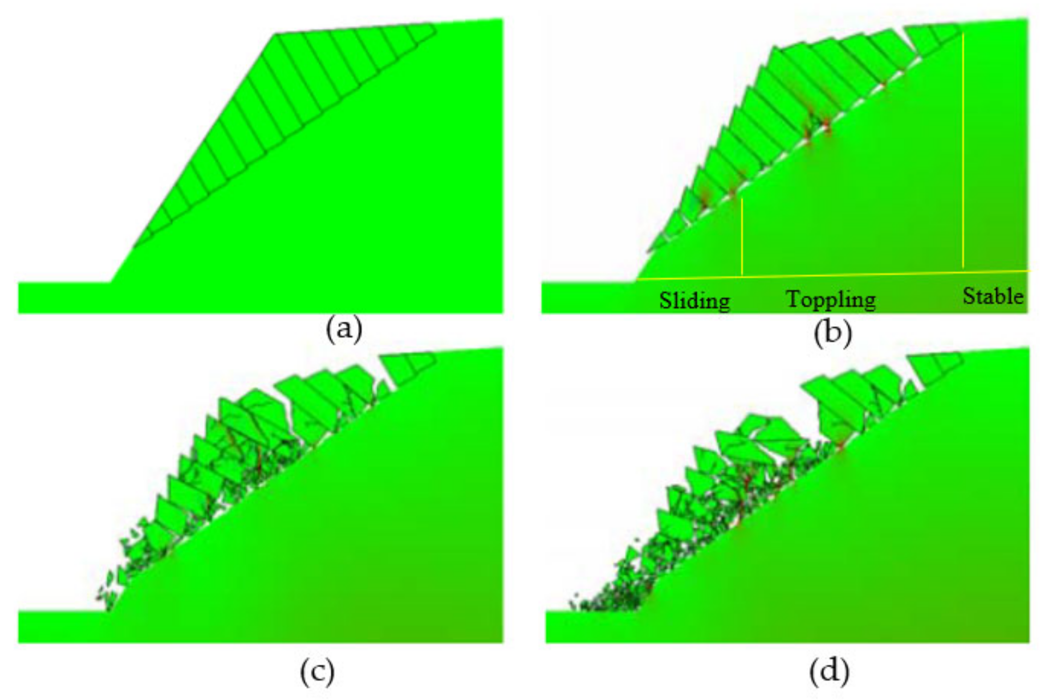
3. Calibration of Hybrid Finite–Discrete Element Method for Modelling the Rock Slope Failure Process

The FDEM has been calibrated by many typical rock mechanism tests, e.g., the Brazilian tensile strength test [27], uniaxial compressive strength test [28], three-point test [26], and four-point test [24]. Those modelling results indicate that the FDEM can effectively model various fracture types, i.e., tensile, shear, and combination failures. To better indicate the capability of the FDEM in modelling the entire rock failure process of a rock slope, the FDEM has been employed to model the typical rock slope failure process [46], and it is even used for the back analysis of the rock slope in which the failure has occurred [21].

Grasselli, Lisjak et al. (2011) modelled the toppling failure of the rock slope, which is one of the main rock slope failure types [46], to calibrate and show the capabilities of the FDEM method in modelling the entire rock failure process of the rock slope. Figure 7 illustrates the temporal sequence of the failure process and the resultant fragmentation of the toppling failure of the rock slope. As can be seen from Figure 7, the toppling rock slope is comprised of multiple columns and those interact on an inclined plane during the rock-toppling failure process. According to Bray and Goodman (1981) [47], the toppling slope can be divided into three sections, i.e., the stable section, sliding section, and toppling section (Figure 7b). Due to the gravity of the columnar blocks, the failure occurs in the toppling and sliding sections, as illustrated in Figure 7b. The blocks slid on the inclined plane in the sliding sections while the blocks slide and rotate in the toppling section. During the interactions of the blocks, many blocks break into smaller blocks and even fragments (Figure 7c). Finally, more fragments are produced and pile on the toe of the slope during the gravity of the blocks interacting with the adjacent blocks (Figure 7c). The rock mass on the stable section is not significantly influenced by the slope failure process, as there is no interaction between adjacent blocks and the force along the sliding face induced by gravity is not big enough to cause the blocks to slide, due to the friction on the discontinuity face.

Sun, Liu et al. (2022) developed the Y-slope to model the entire failure process of rock slopes from initiation and transportation to deposition [19]. The Y-slope is developed based on the Y-code. The Y-slope considered the shear and tensile failure conditions by the implementation of the strength reduction methods. To calibrate the Y-slope, the equilibrium state of a benchmark is modelled. The stress distribution and displacement distribution are illustrated in Figure 8. It finds that both the stress distribution and the displacement follow a layered distribution, which are similar to the typical results of the rock slope at the equilibrium state obtained from commercial software.

Thus, the FDEM can model the transition of the rock slope from continuum to discontinuum through the rock fracture initiation, propagation and sliding, or rotation. In addition, it can effectively demonstrate the stress distribution and displacement distribution.

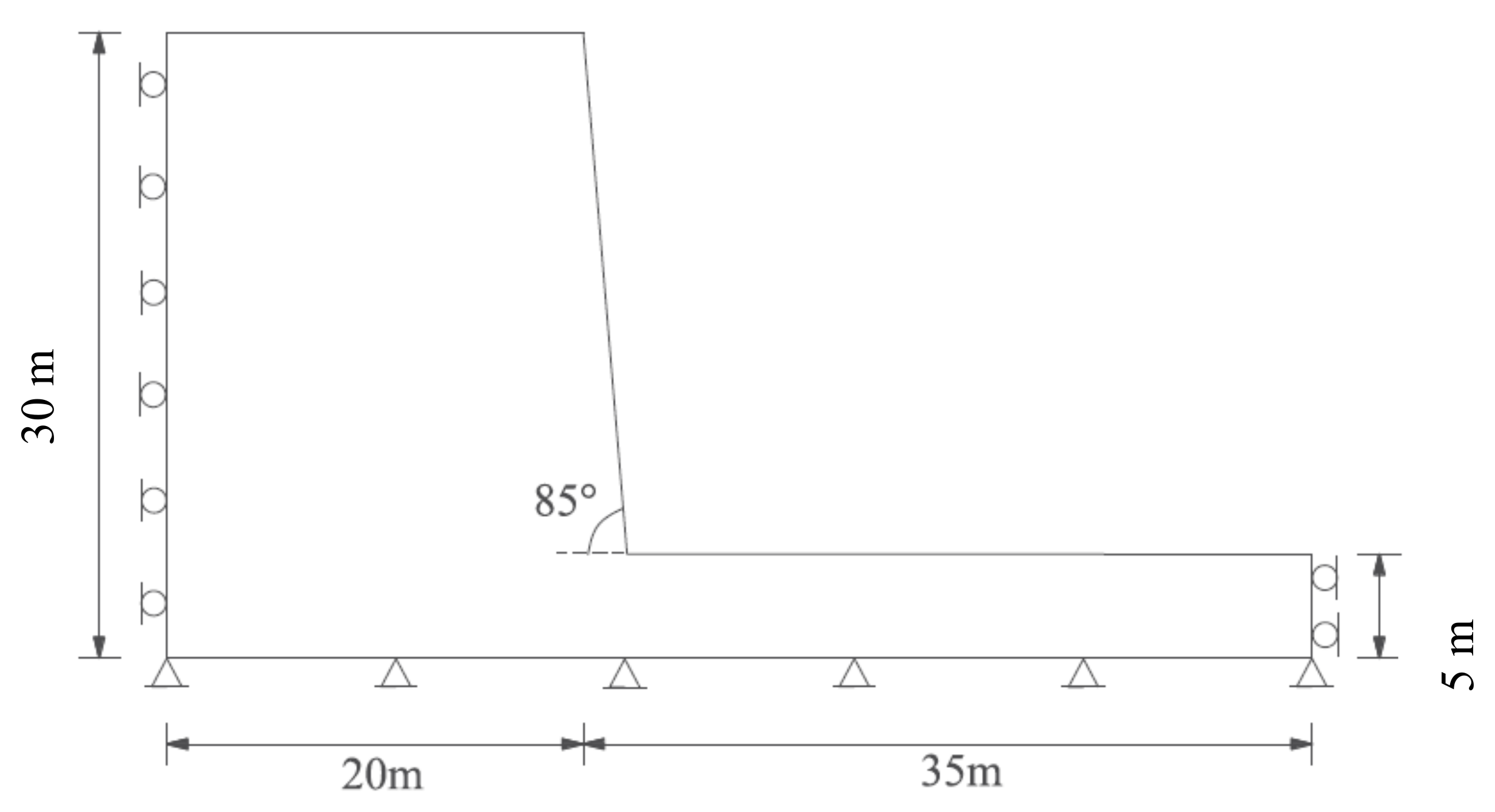
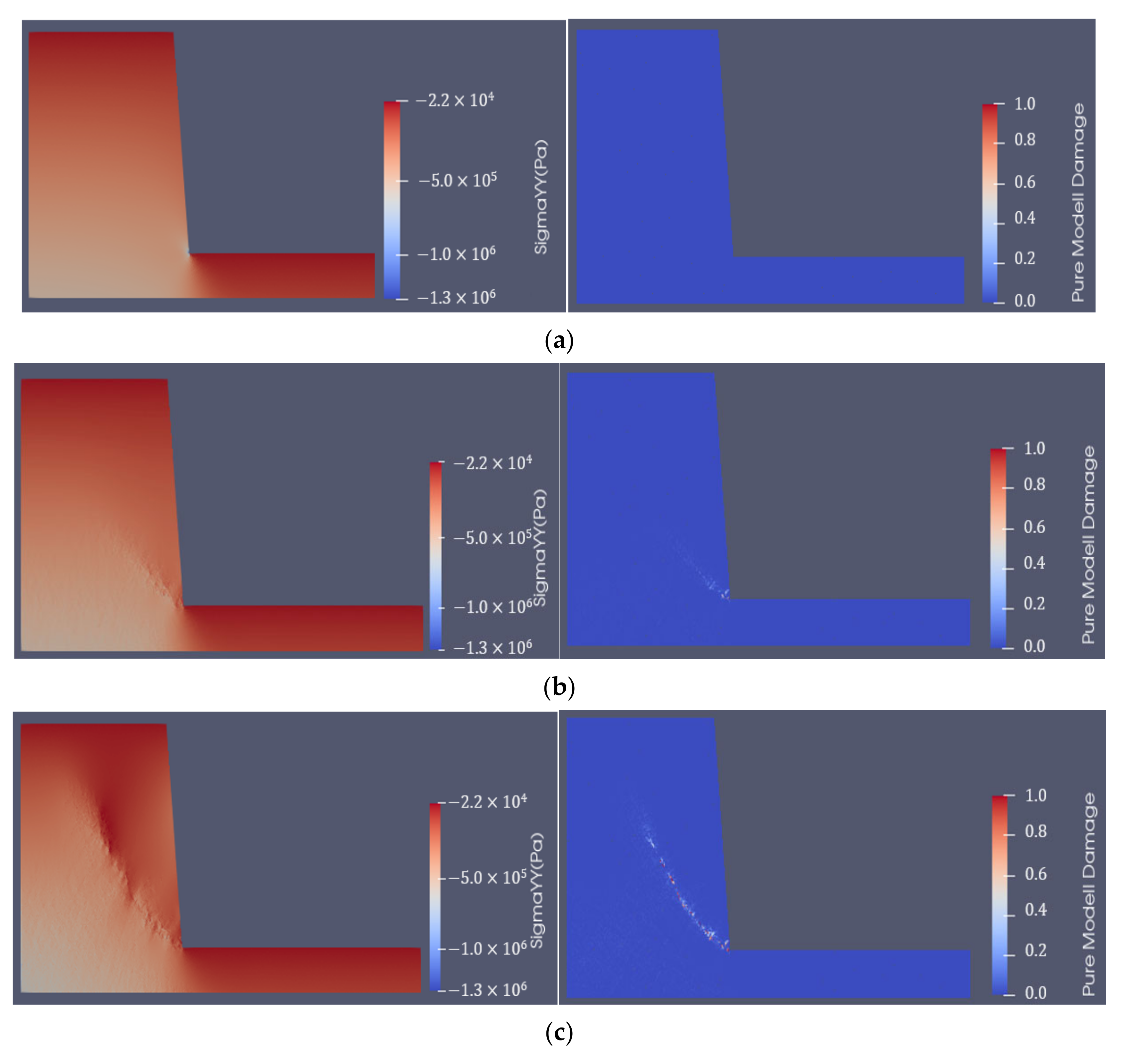
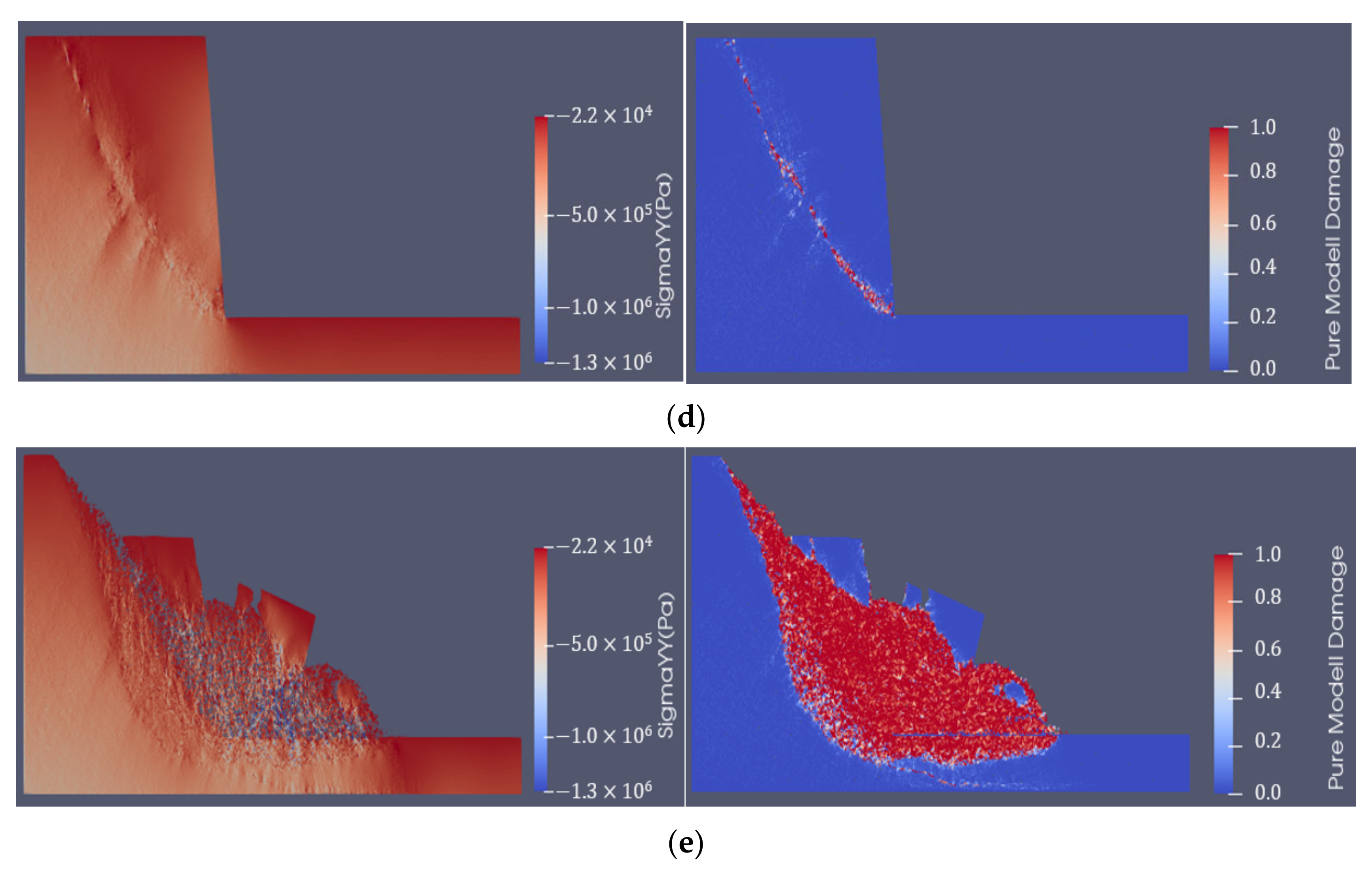
4. Application of the Hybrid Finite–Discrete Element Method in Modelling the Entire Rock Failure Process

Barla, Piovano et al. (2012) simulated two different rock slides observed at the Apletto Mine in Cesana Brianza, Italy [21]. Figure 9 shows the plane view, in which two sections, i.e., Section A and Section B, can be observed. Due to the intensive and persistent rainfall, instability has occurred in Section A. Barla, Piovano et al. (2012) made a back analysis of the side of Section A using FDEM, while the failure process of Section B also is simulated using FDEM.

Figure 10 shows the FDEM modelling of the rock slope failure process of Section A of the Alpetto high rock cut slope. Figure 10a-A illustrates the initial state of the cut slope. It can be seen that the bedding plane in the rock mass is approximately parallel to the slope, which results in the formation of thin slabs. The slabs are generated and move along the discontinuity or the sliding surface (Figure 10a-D). During the movement, the slabs turn to fragments due to the interactions of the slabs with the rock slope discontinuity. Finally, the fragments cover the bottom part of the slope. Figure 10b shows the FDEM modelling of the rock slope sliding process of Section B of the Alpetto high rock cut slope. The FDEM modelled two slopes (Section A and Section B) that are both similar to the high steep-slope failure process. The final fractured rock mass covers the bottom of the slope.

5. Discussion

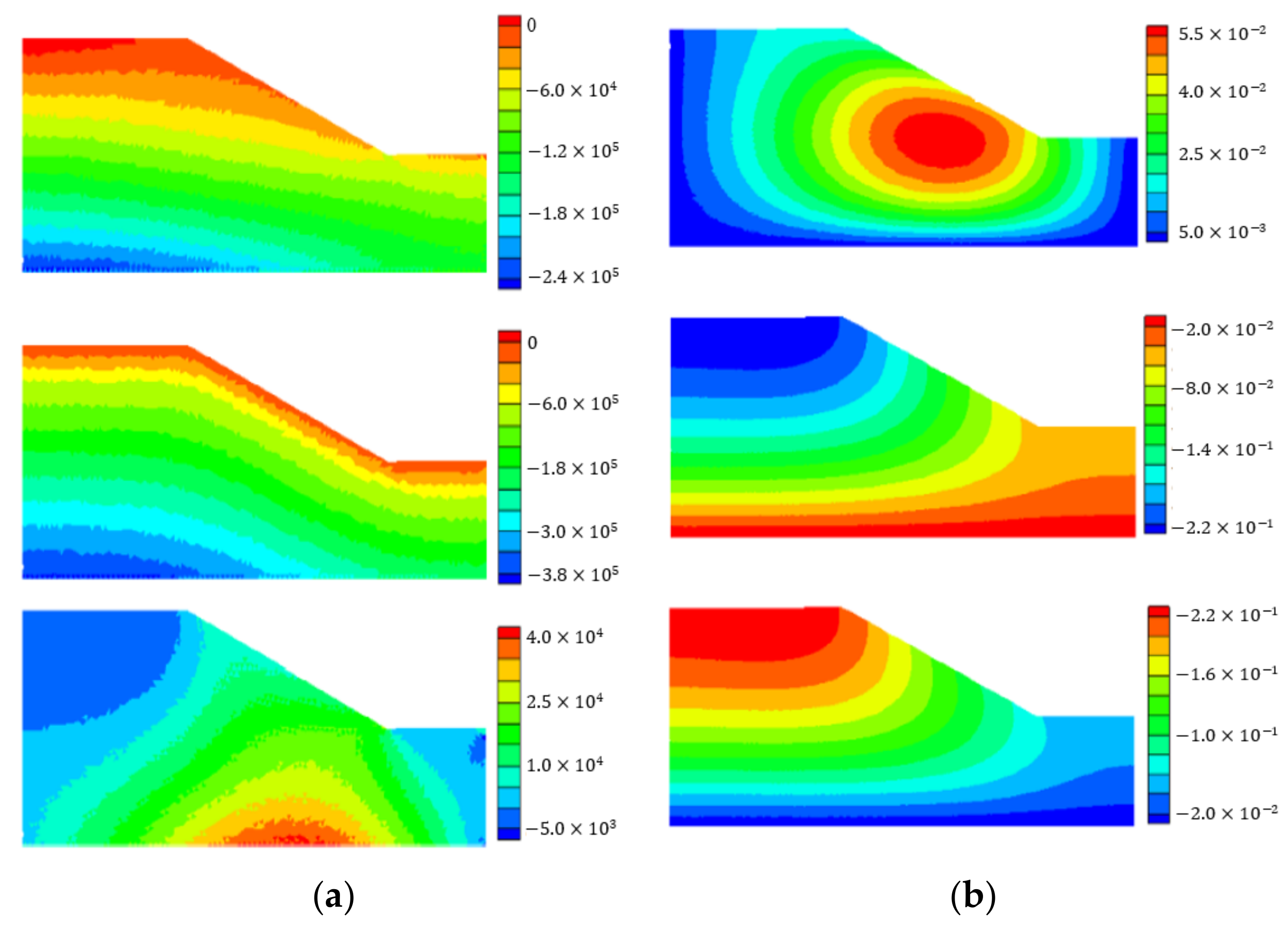
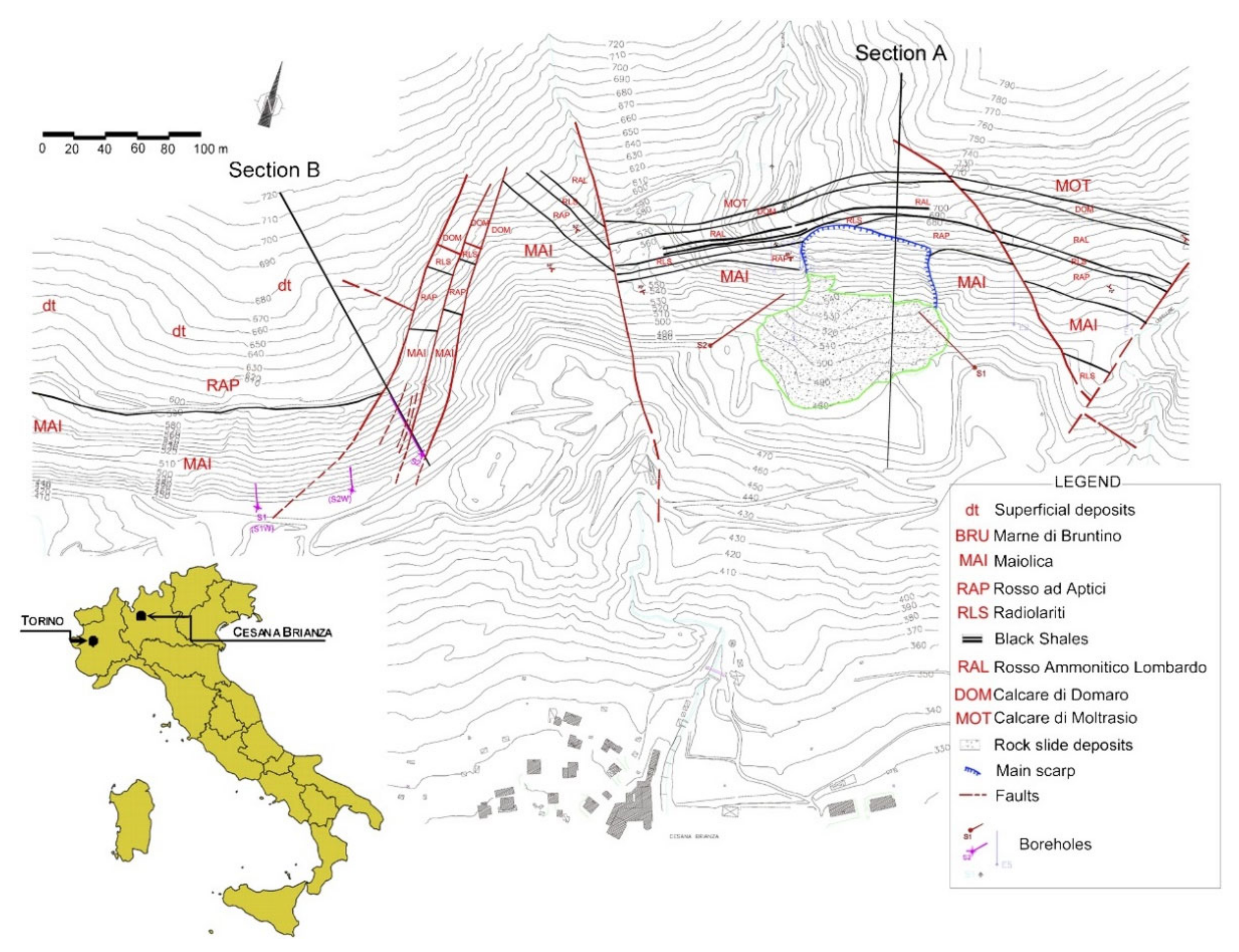
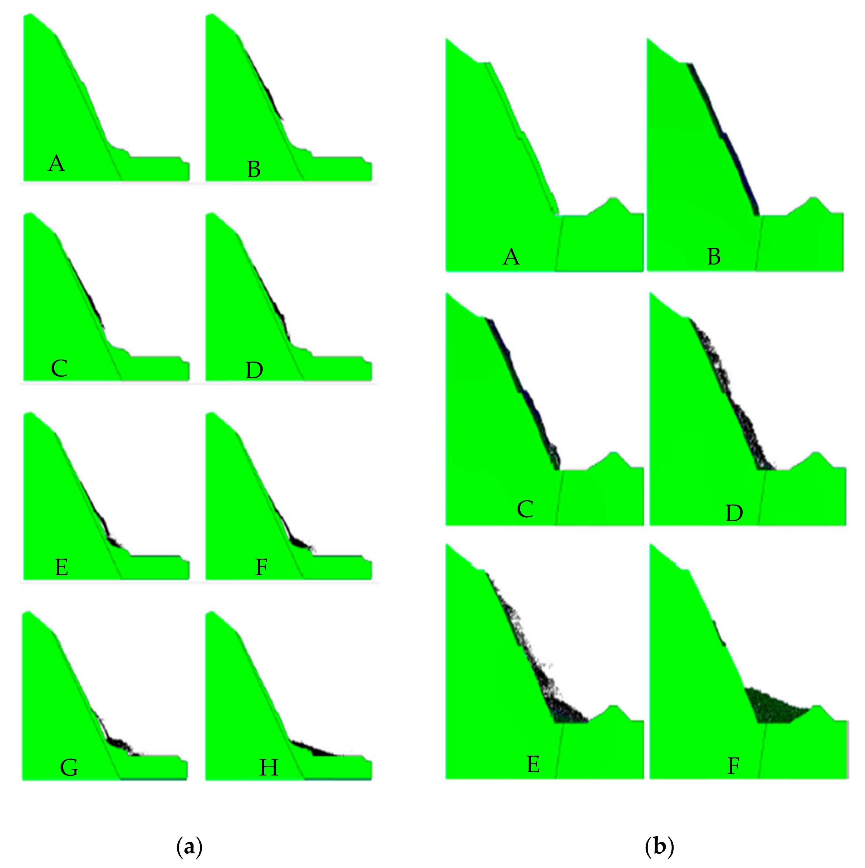
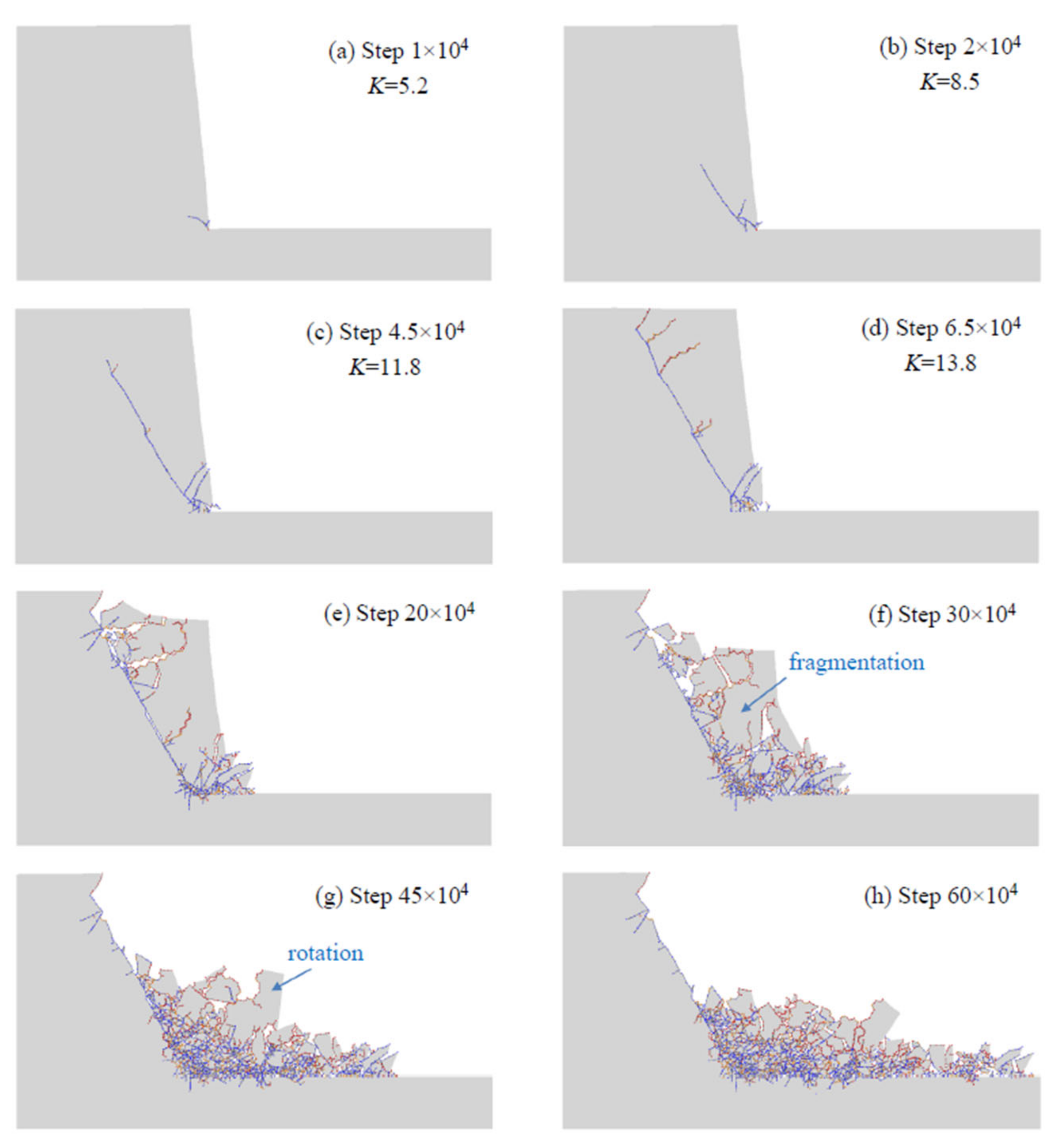
5.1. Discussion on the Numerical Modelling Entire Slope Failure Process

Although many numerical techniques have been applied to model the rock slope failure process [2,6,8,9,18,19,48,49], naturally modelling the entire failure process is still a challenge. The entire rock slope failure process involves continuous displacement and discontinuous interaction. It is also associated with crack initiation, crack propagation, and even the coalescence of the cracks. In the post-failure process, the rock mass may move, rotate, collide, and finally fragment. As it involves continuous behaviours before the failure occurs, and discontinuous behaviour during the post-failure process, an individual continuum or discontinuum method has its limitations in modelling the entire failure process of rock slopes.

Figure 11 illustrates an FDEM method, i.e., Y-slope, which modelled the entire rock slope failure process [19]. Due to the gravity of the rock mass, a crack initiates from the toe of the slope, in which the stress is concentrated (Figure 11a). Then, the crack starts to propagate and reaches the top surface of the slope (Figure 11b–d). Thus, a sliding surface is formed. After that, the rock mass on the sliding surface begins to move along the formed surface (Figure 11e). During the post-failure process, the sliding rock mass rotates, interacts, and collides, which results in massive fragments being produced (Figure 11f). Finally, massive fragments accumulate in the vicinity of the slope toe. The rock slope failure process illustrated in Figure 11 effectively indicates that the FDEM can model the entire slope failure process well, from the continuous behaviours to the discontinuous behaviours.

Figure 12 compares two modelling results for a same toppling failure process. Figure 12a illustrates a toppling failure process modelled using the UDEC, while Figure 12b shows the same failure process modelled using FDEM.

Generally, the modelled results are almost the same in terms of failure formation. As can be seen, the failure initiated from the bottom-three rock blocks, and this caused the instability of the other blocks, except for the two blocks at the top of the sliding discontinuity. Then, the fracture blocks moved along the sliding surface. Thus, the UEDC and the FDEM both can model the toppling failure process well. However, it seems that FDEM has modelled the fracture initiation and propagation better when compared with the UDEC-obtained results in this case, which shows the advantage of the continuum method.

5.2. Discussion on the Advantages and Limitations of the FDEM in Rock Fracture Modelling

As the FDEM is a combined/hybrid continuum and discontinuum method, it takes the advantages of both the continuum method, e.g., FEM, and discontinuum method, e.g., DDA. The continuum method can model the rock initiation well, as well as propagation and coalescence, including the localization of the failure [18], while the discontinuum is good at modelling the sliding of the rocks along the discontinuous surface, as well as the interaction and rotation of the blocks. Thus, the FDEM can model the entire rock slope sliding process, i.e., crack initiation, propagation, coalescence, and the rock bodies’ movements, interactions, and fragmentations. In another word, the FDEM allows for new crack initiation and exiting crack extension, and can model the larger deformation, including rotations.

However, the FDEM also has its limitations. For example, the FDEM requires very specialized input parameters, and the required joint properties are not routinely measured [39]. In addition, the FDEM modelling results are very sensitive to the mesh size and mesh orientation, since the joint element or crack elements are inserted among the finite element boundaries to model the fracture initiation and propagation. Moreover, the FDEM encounters difficulties when simulating failures through intact rock.

Thus, new techniques need to be developed to more naturally model the crack initiation and propagation, and to try to avoid the effects of the mesh size and mesh orientation. Moreover, the crack initiated from the intact rock should be developed as the rock slope sliding process includes not only discontinuous mechanical behaviours but also crack initiation, propagation, and coalescence from intact rock [23,50].

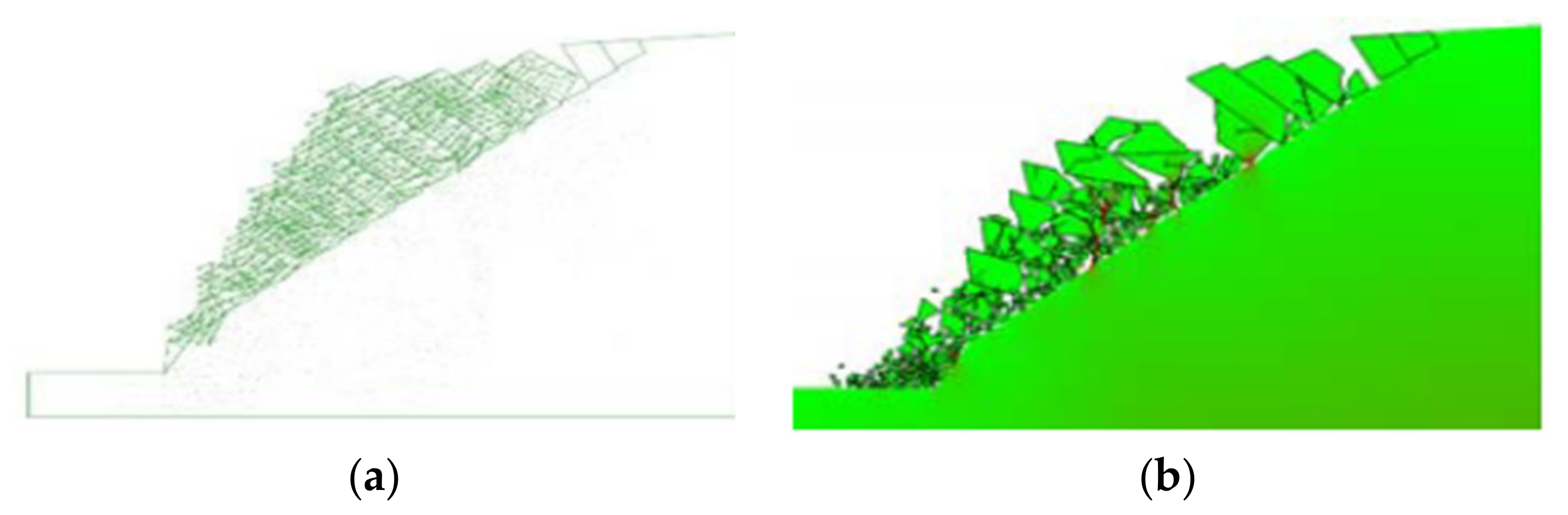
6. New Insight into GPGPU-Parallelized FDEM Modelling of Rock Slope Failure Process

The significance of understanding the mechanism of the rock fracturing process has been widely realized in several fields, e.g., rock slopes and tunnellings, in which the stability is sensitive to the fractures. Numerical methods have been implemented to model the fracture process and the FDEM is considered as a promising tool, as mentioned in the Introduction Section. However, the computing power limited the FDEM, not only with 3D modelling but also in carrying out large-scale 2D modelling with a small mesh size in the past. The recently developed general purpose graphic processing unit (GPGUP) accelerators have dramatically improved this situation. Thus, this section gives a brief insight into the GPGUP-parallelized FDEM in modelling the rock slope failure process.

The FDEM code, i.e., Y-HFDEM, used in this section is originally developed by the authors in reference [51] and has been employed to study the conventional rock mechanism tests [26,27,28], rock blasting in mining production [25], and tunnelling excavation [29,41]. To overcome the computationally expensive issue of Y-HFDEM, the authors Fukuda et al. (2019–2020) [52,53] recently parallelized it on the basis of the GPGPU using a compute-unified device architecture (CUDA) C/C++. The detailed computing performance analysis shows the GPGPU-parallelized HFDEM 2D/3D IDE code can achieve the maximum speedups of 128.6 [53] and 286 [52] times in the case of the 2D and 3D modellings, respectively. More recently, adaptive efficient contact activation [54], mass scaling, the hyperplane separation theorem, and the semi-adaptive contact activation approach [55] have been implemented by the authors to further speed up the GPGPU-parallelized HFDEM, which paves the way for investigating the large-scale rock slope failure process.

The safety factor (SF) has been introduced in the Introduction Section, which is regarded as the key indicator for the stability of a slope. In addition, the safety factor can be obtained by weakening the rock material until the slope fails using the strength reduction method (SRM) [56,57]. For the modelling of the rock slope failure process using GPGUP-parallelized Y-HFDEM, the strength reduction method (SRM) is implemented in the proposed method. Then, a typical rock high slope is modelled to gain insight into the GPGUP-parallelized Y-HFDEM on the rock slope stability analysis. Figure 13 illustrates the geometrical mode, the size of which is the same as in Figure 11 of reference [19].

Table 2. Input parameters for the FDEM high rock slope model.

Properties	Values
Young’s modulus (GPa)	10
Poisson’s ratio	0.25
Density (kg/m3)	2000
Friction angle (degrees)	32
Cohesion (MPa)	1
Tensile strength (MPa)	0.5

gives the input parameters for the FDEM high rock slope model, which are the same as in Figure 11 of reference [19].

The following input parameters in

Table 3. Input parameters for the GPGUP-parallelized Y-HFDEM high rock slope model.

Properties	Values
Mode-I fracture energy (J/m2)	4
Mode-II fracture energy (J/m2)	12
Normal contact penalty (GPa)	100
Tangent contact penalty (GPa)	100
Artificial stiffness penalty (GPa)	1000

are not provided in reference [19] but are chosen following the calibration procedure described by Mohammadnejad et al. (2020) [54].

During the modelling, the gravity of the rock mass is firstly applied to the model and the stress reaches an equilibrium state through implementing a local damping approach. A damping coefficient is incorporated into the constitutive model in the FDEM, which is the so-called critical damping technique, one of the simplest approaches that have been used in many explicit FDEM. However, it was noted that the convergence rate of the critical damping technique is rather poor. Correspondingly, a local damping with a mass scaling technique is implemented into the GPGPU-parallelized HFDEM IDE code following Equation (8).

$${\mathit{M}}^{scale}{\partial }^2\mathit{u}/\partial t^2={\mathit{f}}_{tot}+\alpha \left|\right|{\mathit{f}}_{tot}\left|\right|sgn\left(\mathit{v}\right)$$

(8)

where M^scale is the scaled lumped mass, f_tot is the nodal out-of-balance force, v is the nodal velocity, ||f_tot|| is the absolute value of each component of f_tot, sgn(∙) is the sign function automatically determined by the sign of (∙), and α is the local damping coefficient. Please refer to Fukuda et al. (2019) [53] for the implementation of the local damping method in detail. This process is completely different from that implemented in reference [19].

During the process, no fracture is allowed, since cohesive elements have not been inserted. After that, cohesive elements are inserted and static equilibrium is achieved. As the strength reduction method (SRM) is implemented in the proposed method, an iterative process begins. The strength parameters are reduced and re-arranged into the model. Then, a stress equilibrium state will be achieved again. The iterative process will not stop until the slope becomes unstable. Figure 14 illustrates a typical rock slope failure process using the proposed method with the implementation of the SRM. The left part of Figure 14 indicates the stress distribution while the right part shows the fracture initiation and propagation. Figure 14a indicates the stress equilibrium state after the gravity of the rock mass is applied to the model. The stress concentration can be observed at the toe of the slope, where fractures initiate (Figure 14b). Then, the fractures propagate into the slope (Figure 14c) and form a sliding failure surface (Figure 14d). The rock mass slides along the newly formed sliding surface. Due to the sliding, rotation, and colliding, the rock mass breaks into fragments and finally piles at the lower bench of the slope (Figure 14e). Thus, the GPGUP-parallelized Y-HFDEM can effectively model the entire slope failure evolution process due to the implementation of the SRM in the proposed method.

7. Conclusions

The stability of rock slopes plays a significant role in many geotechnical engineering projects. To avoid the catastrophes induced by the instability of the rock slopes and to optimize the slopes for reliability, many techniques have been developed, which can be classified into convention methods and numerical methods. The limited analysis method is the most popular and widely used conventional technique, which can provide the factor of the safety of the rock slopes. However, the limited method is mostly limited to analyzing the planar failure and wedge failure, and it is beyond the capability of the limited analysis method for complicated failure types. With the fast development of computation techniques, numerical techniques are employed to analyze the stability of the rock slopes. In general, the numerical techniques mainly include three types, i.e., the continuum method, discontinuum method, and the combined/hybrid continuum–discontinuum method. Both the continuum and discontinuum methods can model the slope failure process. However, due to the material assumptions, i.e., the continuum material or discontinuum material, the continuum or discontinuum methods have limitations in modelling the entire failure process. The continuum–discontinuum methods combined the advantages and avoid the disadvantages of the continuum methods and the discontinuum methods. Thus, a representative continuum–discontinuum method, i.e., the combined/hybrid finite–discrete element method (FDEM), is reviewed, calibrated, and then implemented in the rock slope stability analysis in this article. The fundamental principles of the FDEM are introduced. Compared with continuum methods and discontinuum methods, one of the most distinct is that the FDEM can model the transition from continuum to discontinum. Therefore, the FDEM can model the entire slope sliding process naturally. This research paper gives a detailed explanation of this distinction, i.e., the transition from continuum to discontinuum. In addition, the three fracture modes that make the FDEM able to model the transition from continuum to discontinuum through fracture and fragmentation are introduced. The calibration of the FDEM is essential to show its abilities in rock slope failure modelling. The authors reviewed the typical slope failure process modelled using the FDEM to calibrate the proposed method. The stress and displacement distributions modelled by the FDEM are similar to those obtained by commercial software. Moreover, the FDEM can obtain the fracture initiation, the interaction of the rock bodies, and the rock wedges sliding along the failure surface. After that, the employment of the FDEM for the back analysis of the rock slope failure and predicting the rock failure using FDEM is given. Finally, the GPGUP-parallelized FDEM with the implementation of the strength reduction method (SRM) is introduced and employed to model the rock slope failure process to gain insight into the recent advance in FDEM techniques. On the basis of the review research, it is concluded that:

• The FDEM can effectively model the entire rock slope failure process from the fracture initiation, wedge sliding, and fragmentation due to the transition from the continuum to discontinuum technique implemented in the FDEM;
• The continuum or the discontinuum methods have their limitations in naturally modelling the entire rock failure process. However, the distinctive character, i.e., the transition from continuum to discontinuum, means that the FDEM can effectively model the natural failure process for the rock slopes, even without any failure modes implemented in the proposed method;
• The GPGUP-parallelized FDEM with the implementation of SRM is a promising technique in the back analysis and prediction of the slope failure process, as it combined the advantages of the continuum methods and discontinuum methods, and it can naturally model the transition for rock from continuum to discontinuum through fracture and fragmentations.

References

1. Wyllie, D.C.; Mah, C. Rock Slope Engineering; CRC Press: Boca Raton, FL, USA, 2004. [Google Scholar]
2. Tang, H.; Yong, R.; Ez Eldin, M.A.M. Stability analysis of stratified rock slopes with spatially variable strength parameters: The case of Qianjiangping landslide. Bull. Eng. Geol. Environ. 2017, 76, 839–853. [Google Scholar] [CrossRef]
3. Norrish, N.I.; Wyllie, D.C. Landslides: Investigation and Mitigation. Chapter 15—Rock Slope Stability Analysis; Transportation Research Board: Washington, DC, USA, 1996. [Google Scholar]
4. Stead, D.; Wolter, A. A critical review of rock slope failure mechanisms: The importance of structural geology. J. Struct. Geol. 2015, 74, 1–23. [Google Scholar] [CrossRef]
5. Abramson, L.W.; Lee, T.S.; Sharma, S.; Boyce, G.M. Slope Stability and Stabilization Methods; John Wiley & Sons: Hoboken, NJ, USA, 2001. [Google Scholar]
6. Jin, Y.-F.; Yin, Z.-Y.; Yuan, W.-H. Simulating retrogressive slope failure using two different smoothed particle finite element methods: A comparative study. Eng. Geol. 2020, 279, 105870. [Google Scholar] [CrossRef]
7. Lv, Z.Q.; Wang, B.S.; Zhang, X.X. The PFC2DSimulation of the Slope Stability. In Advanced Materials Research; Trans Tech Publications Ltd.: Bäch SZ, Switzerland, 2015; pp. 240–243. [Google Scholar]
8. Yang, Y.; Xu, D.; Liu, F.; Zheng, H. Modeling the entire progressive failure process of rock slopes using a strength-based criterion. Comput. Geotech. 2020, 126, 103726. [Google Scholar] [CrossRef]
9. Shen, J.; Karakus, M. Three-dimensional numerical analysis for rock slope stability using shear strength reduction method. Can. Geotech. J. 2014, 51, 164–172. [Google Scholar] [CrossRef]
10. Yodsomjai, W.; Keawsawasvong, S.; Thongchom, C.; Lawongkerd, J. Undrained stability of unsupported conical slopes in two-layered clays. Innov. Infrastruct. Solut. 2021, 6, 15. [Google Scholar] [CrossRef]
11. Yodsomjai, W.; Keawsawasvong, S.; Senjuntichai, T. Undrained stability of unsupported conical slopes in anisotropic clays based on anisotropic undrained shear failure criterion. Transp. Infrastruct. Geotechnol. 2021, 8, 557–568. [Google Scholar] [CrossRef]
12. Yodsomjai, W.; Keawsawasvong, S.; Likitlersuang, S. Stability of unsupported conical slopes in Hoek-Brown rock masses. Transp. Infrastruct. Geotechnol. 2021, 8, 279–295. [Google Scholar] [CrossRef]
13. Li, A.-J.; Lyamin, A.; Merifield, R. Seismic rock slope stability charts based on limit analysis methods. Comput. Geotech. 2009, 36, 135–148. [Google Scholar] [CrossRef]
14. Li, A.J.; Merifield, R.S.; Lyamin, A.V. Stability charts for rock slopes based on the Hoek-Brown failure criterion. Int. J. Rock Mech. Min. Sci. 2008, 45, 689–700. [Google Scholar] [CrossRef]
15. Jing, L. A review of techniques, advances and outstanding issues in numerical modelling for rock mechanics and rock engineering. Int. J. Rock Mech. Min. Sci. 2003, 40, 283–353. [Google Scholar] [CrossRef]
16. Jiang, M.; Murakami, A. Distinct element method analyses of idealized bonded-granulate cut slope. Granul. Matter 2012, 14, 393–410. [Google Scholar] [CrossRef]
17. Zhang, Y.; Xu, Q.; Chen, G.; Zhao, J.X.; Zheng, L. Extension of discontinuous deformation analysis and application in cohesive-frictional slope analysis. Int. J. Rock Mech. Min. Sci. 2014, 70, 533–545. [Google Scholar] [CrossRef]
18. Tang, S.; Huang, R.; Tang, C.; Liang, Z.; Heap, M. The failure processes analysis of rock slope using numerical modelling techniques. Eng. Fail. Anal. 2017, 79, 999–1016. [Google Scholar] [CrossRef]
19. Sun, L.; Liu, Q.; Abdelaziz, A.; Tang, X.; Grasselli, G. Simulating the entire progressive failure process of rock slopes using the combined finite-discrete element method. Comput. Geotech. 2022, 141, 104557. [Google Scholar] [CrossRef]
20. Zhou, W.; Yuan, W.; Ma, G.; Chang, X.L. Combined finite-discrete element method modeling of rockslides. Eng. Comput. 2016, 33, 1530–1559. [Google Scholar] [CrossRef]
21. Barla, M.; Piovano, G.; Grasselli, G. Rock slide simulation with the combined finite-discrete element method. Int. J. Geomech. 2012, 12, 711–721. [Google Scholar] [CrossRef]
22. Mahabadi, O.; Grasselli, G.; Munjiza, A. Y-GUI: A graphical user interface and pre-processor for the combined finite-discrete element code, Y2D, incorporating material heterogeneity. Comput. Geosci. 2010, 36, 241–252. [Google Scholar] [CrossRef]
23. Eberhardt, E.; Stead, D.; Coggan, J.S. Numerical analysis of initiation and progressive failure in natural rock slopes—The 1991 Randa rockslide. Int. J. Rock Mech. Min. Sci. 2004, 41, 69–87. [Google Scholar] [CrossRef]
24. An, H.; Wu, S.; Liu, H.; Wang, X. Hybrid Finite-Discrete Element Modelling of Various Rock Fracture Modes during Three Conventional Bending Tests. Sustainability 2022, 14, 592. [Google Scholar] [CrossRef]
25. An, H.; Song, Y.; Liu, H.; Han, H. Combined Finite-Discrete Element Modelling of Dynamic Rock Fracture and Fragmentation during Mining Production Process by Blast. Shock. Vib. 2021, 2021, 6622926. [Google Scholar] [CrossRef]
26. An, H.; Song, Y.; Liu, H. FDEM Modelling of Rock Fracture Process during Three-Point Bending Test under Quasistatic and Dynamic Loading Conditions. Shock. Vib. 2021, 2021, 5566992. [Google Scholar] [CrossRef]
27. An, H.; Liu, H.; Han, H. Hybrid finite–discrete element modelling of rock fracture process in intact and notched Brazilian disc tests. Eur. J. Environ. Civ. Eng. 2021, 1–34. [Google Scholar] [CrossRef]
28. Huaming, A.; Hongyuan, L.; Han, H. Hybrid finite-discrete element modelling of rock fracture during conventional compressive and tensile strength tests under quasi-static and dynamic loading conditions. Lat. Am. J. Solids Struct. 2020, 17, 1–32. [Google Scholar]
29. An, H.; Liu, H.; Han, H. Hybrid Finite-Discrete Element Modelling of Excavation Damaged Zone Formation Process Induced by Blasts in a Deep Tunnel. Adv. Civ. Eng. 2020, 2020, 7153958. [Google Scholar] [CrossRef]
30. An, H.; Liu, H.; Han, H.; Zheng, X.; Wang, X. Hybrid finite-discrete element modelling of dynamic fracture and resultant fragment casting and muck-piling by rock blast. Comput. Geotech. 2017, 81, 322–345. [Google Scholar] [CrossRef]
31. Mohammadnejad, M.; Liu, H.; Chan, A.; Dehkhoda, S.; Fukuda, D. An overview on advances in computational fracture mechanics of rock. Geosystem Eng. 2021, 24, 206–229. [Google Scholar] [CrossRef]
32. Bradley, A.L. Investigating the Influence of Mechanical Anisotropy on the Fracturing Behavior of Brittle Clay Shales with Application to Deep Geological Repositories. In Proceedings of the 13th ISRM International Congress of Rock Mechanics, Montreal, QC, Canada, 10–13 May 2015. [Google Scholar]
33. Zhao, Q.; Lisjak, A.; Mahabadi, O.; Liu, Q.; Grasselli, G. Numerical simulation of hydraulic fracturing and associated microseismicity using finite-discrete element method. J. Rock Mech. Geotech. Eng. 2014, 6, 574–581. [Google Scholar] [CrossRef] [Green Version]
34. Lukas, T.; Schiava D’Albano, G.G.; Munjiza, A. Space decomposition based parallelization solutions for the combined finite–discrete element method in 2D. J. Rock Mech. Geotech. Eng. 2014, 6, 607–615. [Google Scholar] [CrossRef] [Green Version]
35. Jing, L.; Hudson, J. Numerical methods in rock mechanics. Int. J. Rock Mech. Min. Sci. 2002, 39, 409–427. [Google Scholar] [CrossRef]
36. Munjiza, A. The Combined Finite-Discrete Element Method; Wiley Online Library: Hoboken, NJ, USA, 2004. [Google Scholar]
37. Munjiza, A.; Xiang, J.; Garcia, X.; Latham, J.; D’Albano, G.S.; John, N. The virtual geoscience workbench, VGW: Open source tools for discontinuous systems. Particuology 2010, 8, 100–105. [Google Scholar] [CrossRef]
38. Vyazmensky, A.; Stead, D.; Elmo, D.; Moss, A. Numerical Analysis of Block Caving-Induced Instability in Large Open Pit Slopes: A Finite Element/Discrete Element Approach. Rock Mech. Rock Eng. 2010, 43, 21–39. [Google Scholar] [CrossRef]
39. Styles, T. Numerical Modelling and Analysis of Slope Stability within Fracture Dominated Rock Masses; University of Exeter: Exeter, UK, 2009. [Google Scholar]
40. Tatonea, B.; Grassellia, G. A calibration procedure for two-dimensional laboratory-scale hybrid finite-discrete element simulations. Int. J. Rock Mech. Min. Sci. 2015, 75, 56–72. [Google Scholar] [CrossRef]
41. Han, H.; Fukuda, D.; Liu, H.; Salmi, E.F.; Sellers, E.; Liu, T.; Chan, A. Combined finite-discrete element modelling of rock fracture and fragmentation induced by contour blasting during tunnelling with high horizontal in-situ stress. Int. J. Rock Mech. Min. Sci. 2020, 127, 104214. [Google Scholar] [CrossRef]
42. Mohammadi, S. Discontinuum Mechanics: Using Finite and Discrete Elements; WIT Press: Southampton, UK, 2003. [Google Scholar]
43. Munjiza, A.; Andrews, K.; White, J. Combined single and smeared crack model in combined finite-discrete element analysis. Int. J. Numer. Methods Eng. 1999, 44, 41–57. [Google Scholar] [CrossRef]
44. Liu, H.; Kou, S.; Lindqvist, P.-A.; Tang, C. Numerical studies on the failure process and associated microseismicity in rock under triaxial compression. Tectonophysics 2004, 384, 149–174. [Google Scholar] [CrossRef]
45. Xiang, J.; Munjiza, A.; Latham, J.P. Finite strain, finite rotation quadratic tetrahedral element for the combined finite–discrete element method. Int. J. Numer. Methods Eng. 2009, 79, 946–978. [Google Scholar] [CrossRef]
46. Grasselli, G.; Lisjak, A.; Mahabadi, O.; Tatone, B. Slope Stability Analysis Using a Hybrid Finite-Discrete Element Method Code (EMDEM). In Proceedings of the 12th ISRM Congress, Beijing, China, 18–21 October 2011. [Google Scholar]
47. Bray, J.W.; Goodman, R.E. The theory of base friction models. Int. J. Rock Mech. Min. Sci. Geomech. Abstr. 1981, 18, 453–468. [Google Scholar] [CrossRef]
48. Zhu, C.; He, M.C.; Karakus, M.; Cui, X.B.; Tao, Z.G. Investigating Toppling Failure Mechanism of Anti-dip Layered Slope due to Excavation by Physical Modelling. Rock Mech. Rock Eng. 2020, 53, 5029–5050. [Google Scholar] [CrossRef]
49. Zheng, W.; Zhuang, X.; Tannant, D.D.; Cai, Y.; Nunoo, S. Unified continuum/discontinuum modeling framework for slope stability assessment. Eng. Geol. 2014, 179, 90–101. [Google Scholar] [CrossRef]
50. Wong, L.N.Y.; Wu, Z. Application of the numerical manifold method to model progressive failure in rock slopes. Eng. Fract. Mech. 2014, 119, 1–20. [Google Scholar] [CrossRef]
51. Liu, H.Y.; Kang, Y.M.; Lin, P. Hybrid finite–discrete element modeling of geomaterials fracture and fragment muck-piling. Int. J. Geotech. Eng. 2015, 9, 115–131. [Google Scholar] [CrossRef]
52. Fukuda, D.; Mohammadnejad, M.; Liu, H.; Zhang, Q.; Zhao, J.; Dehkhoda, S.; Chan, A.; Kodama, J.-I.; Fujii, Y. Development of a 3D Hybrid Finite-Discrete Element Simulator Based on GPGPU-Parallelized Computation for Modelling Rock Fracturing Under Quasi-Static and Dynamic Loading Conditions. Rock Mech. Rock Eng. 2020, 53, 1079–1112. [Google Scholar] [CrossRef]
53. Fukuda, D.; Mohammadnejad, M.; Liu, H.Y.; Dehkhoda, S.; Chan, A.; Cho, S.H.; Min, G.J.; Han, H.; Kodama, J.; Fujii, Y. Development of a GPGPU-parallelized hybrid finite-discrete element method for modeling rock fracture. Int. J. Numer. Anal. Methods Geomech. 2019, 43, 1797–1824. [Google Scholar] [CrossRef]
54. Mohammadnejad, M.; Fukuda, D.; Liu, H.Y.; Dehkhoda, S.; Chan, A. GPGPU-parallelized 3D combined finite-discrete element modelling of rock fracture with adaptive contact activation approach. Comput. Part. Mech. 2020, 7, 849–867. [Google Scholar] [CrossRef]
55. Fukuda, D.; Liu, H.; Zhang, Q.; Zhao, J.; Kodama, J.-I.; Fujii, Y.; Chan, A.H.C. Modelling of dynamic rock fracture process using the finite-discrete element method with a novel and efficient contact activation scheme. Int. J. Rock Mech. Min. Sci. 2021, 138, 104645. [Google Scholar] [CrossRef]
56. Cheng, Y.M.; Lansivaara, T.; Wei, W.B. Two-dimensional slope stability analysis by limit equilibrium and strength reduction methods. Comput. Geotech. 2007, 34, 137–150. [Google Scholar] [CrossRef]
57. Wei, Y.; Jiaxin, L.; Zonghong, L.; Wei, W.; Xiaoyun, S. A strength reduction method based on the Generalized Hoek-Brown (GHB) criterion for rock slope stability analysis. Comput. Geotech. 2020, 117, 103240. [Google Scholar] [CrossRef]
Figure 1. Examples of rock slopes (from reference [1]). (a) Rock slope in Hong Kong. (b) Palabora open-pit mine.
Sustainability 14 04896 g001
Figure 2. The main failure types for rock slopes (from references [3,4]). (a) General plane failure sketch (from references [3,4]). (b) Wedge failure sketch (from references [3,4]). (c) Toppling failure sketch (from reference [3]). (d) Circular failure (from reference [3]).
Sustainability 14 04896 g002
Figure 4. The rock mass with cracks and its equivalent numerical model [19]: (a) rock mass (from reference [19]); (b) FDEM model (from reference [19]).
Sustainability 14 04896 g004
Figure 5. Contact force due to penetration [26].
Sustainability 14 04896 g005
Figure 6. Transition from continuum to discontinuum [24,28]: (a) Tension fracture (pure Mode-I fracture (left parts)) and shear fracture (pure Mode-II fracture) (from reference [28]); (b) mixed tensile–shear fracture from (from reference [27]).
Sustainability 14 04896 g006aSustainability 14 04896 g006b
Figure 7. Toppling failure process of the rock slope modelling using FDEM (from reference [46]). (a) Initial state; (b) sliding along the discontinuity surface; (c) interaction between rock blocks; (d) piling to the toe of the slope.
Sustainability 14 04896 g007
Figure 8. FDEM modelling of stress distribution and displacement destitution of the equilibrium state of a benchmark (from reference [19]). (a) Stress distribution; (b) displacement distribution.
Sustainability 14 04896 g008
Figure 9. Plane view of the Alpetto Mine in Northern Italy (from reference [21]).
Sustainability 14 04896 g009
Figure 10. FDEM modelling of rock slope sliding process of the Alpetto high rock cut slope (from reference [21]). (a) Section A; (b) Section B.
Sustainability 14 04896 g010
Figure 11. FDEM modelling of the entire rock slope failure process [19].
Sustainability 14 04896 g011
Figure 12. Comparison of the slope failure process modelled by: (a) the UDEC; (b) the FDEM (from reference [46]).
Sustainability 14 04896 g012
Figure 13. Geometrical model of high rock slope (from reference [19]).
Sustainability 14 04896 g013
Figure 14. GPGUP-parallelized Y-HFDEM IDE modelling of rock slope failure process. (a) Stress equilibrium state; (b) 3 s; (c) 5 s; (d) 10 s; (e) 25 s.
Sustainability 14 04896 g014aSustainability 14 04896 g014b