Article

Impact of Industrial Agglomeration on China’s Residents’ Consumption

School of Business and Economics, Universiti Putra Malaysia, Kuala Lumpur 43400, Malaysia
*
Authors to whom correspondence should be addressed.
Sustainability 2022, 14(7), 4364; https://doi.org/10.3390/su14074364
Submission received: 24 February 2022 / Revised: 19 March 2022 / Accepted: 4 April 2022 / Published: 6 April 2022

Abstract

:
Residents’ consumption is a good indicator of people’s livelihoods and one of the motivations driving economic growth. There are many studies on the influencing factors of residents’ consumption; however, few have studied the effects of industrial agglomeration on residents’ consumption, and even fewer have studied the spatial correlation of residents’ consumption. The goal of this paper is to research the impact of China’s manufacturing industrial agglomeration on residents’ consumption from a spatial perspective. Using data on China’s 31 provinces from 2003 to 2019 and the spatial Durbin model, our results show that the manufacturing industrial agglomeration and residents’ consumption present an inverted “U-shape” relationship and that different regions show different effects. Industrial agglomeration in the eastern region is relatively high and has a restraining effect on residents’ consumption, while industrial agglomeration in the central and western regions is at an early stage and promotes residents’ consumption. Therefore, different regions should adopt different industrial agglomeration policies.

1. Introduction

The current international environment is not very optimistic due to the outbreak of COVID-19 in December 2019, which generated a global panic [1] and attracted considerable media attention [2]. It caused much of the world’s economy to halt [3] and significantly affected many trade activities and residents’ lives with widespread lockdowns and restrictions to prevent further infections. The deterioration of the international economic environment has severely impacted China’s economic development, which relies on exports to drive economic growth. Considering the current and future epidemics, international trade will likely be less prosperous than before, and China’s exports may continue to decline, which means that China will need to rely more on domestic demand to drive economic growth in the future. The authors of [4] suggested that there is an urgency to change from an investment-driven to a consumption-led economic development model in China in order to pursue sustainable and balanced economic development.
In the economic growth model of China, which is reliant on investment and exports, the financial crisis of 2008 and the subsequent anti-globalization wave also caused a sharp drop in investment across the society. During this time, the expansion of residents’ consumption became a key driver of China’s economic growth. In addition, China’s economy is transitioning from its initial development stage to an intermediate or higher development stage. The speed of economic development in this transitional stage depends, to a certain extent, on the extent of consumption; therefore, grasping the consumer demand of Chinese residents is particularly critical. Jie Li et al. [5] and L. Li and Zhu [6] explained that consumption is gradually becoming an important driving force for economic development in China. Promoting the growth of residents’ consumption is a major concern for both policymakers and academics. Many scholars have already given solutions to the problem of expanding consumption, but there are few studies on how industrial agglomeration affects residents’ consumption, and thus far, no clear conclusions have been drawn. Moreover, existing studies on industrial agglomeration and residents’ consumption have mainly focused on urban and rural areas, with few regional studies on the east, center, and west of China. Song et al. [7] proposed that the impact of industrial agglomeration on consumption in urban and rural residents is mainly due to the scale effect, the radiation effect, and the spillover effect of industrial agglomeration. Some scholars have empirically tested whether industrial agglomeration can increase the recognition of regional products and the income level of residents [8], improve product quality [9], and enhance product innovation [10], thereby expanding the types of goods and promoting an increase in residents’ consumption.
China’s policy of developing the east first has led to industrial agglomerations that are concentrated in the eastern region. This policy has caused China’s economy to develop rapidly, but has also led to a spatial imbalance in residents’ consumption, especially between the east, center, and west of China [11]. The emergence of a regional consumption imbalance is inseparable from China’s policies and industrial agglomeration. Kozyreva et al. [12] proposed that the term “consumption” is connected to such terms as “justice” and “equality”. They think that equality of consumption is a source of social wellbeing and inequality of consumption is a more explicit representation of the differences in the wellbeing of different families and socioeconomic groups than inequality of income. Therefore, this research on the impact of industrial agglomeration on regional residents’ consumption also focuses on people’s livelihood, which is a very valuable research field.
The contribution of this paper is as follows. Previous studies have mainly focused on the impacts of industrial agglomeration on economic growth and not residents’ consumption. However, the difference in regional residents’ consumption may better reflect people’s livelihood and equity than economic growth. Industrial agglomeration is an indispensable plan for the development of a country or region, which may eventually lead to equal or unequal regional consumption. Therefore, studying the effect of industrial agglomeration on residents’ consumption is beneficial to the development of the national livelihood and the happiness of people across the world. This paper will adopt the dynamic spatial Durbin model (DSDM) to analyze the effect of industrial agglomeration on residents’ consumption in China from 2003 to 2019. In the past, scholars rarely combined the spatial and temporal effects of residents’ consumption in China. However, residents’ consumption in neighboring regions will have spatial correlations and spatial spillover effects [13,14]. In addition, theoretically, there is a serial dependence in residents’ consumption in different years; for example, last year’s personal consumption expenditure will affect this year’s personal consumption expenditure. Considering the above problems, the dynamic SDM is a better model choice because it can take into account the spatial dependence and serial dependence of variables.

2. Literature Review

2.1. Industrial Agglomeration

At the end of the 19th century, Marshall [15] began to pay attention to the economic phenomenon of industrial agglomeration. He proposed two important concepts, namely, the “internal economy” and “external economy”. Since Marshall, industrial agglomeration has attracted more and more attention from scholars. The concepts of an “industrial concentration zone” and “agglomeration economies” were first proposed and used by Weber [16]. Porter [17] was the first to use “industrial agglomeration” to analyze cluster phenomena. Krugman [18] put forward that geographic agglomeration and specialization produce economies of scale, which, in turn, attract more companies to agglomerate and form industrial agglomerations. He and Zhang [19] think that industrial agglomeration, as a special form of industrial spatial organization in the process of economic and social development, is an important carrier of regional production activities and environmental governance. Some scholars have summarized that industrial agglomeration can reduce transaction and transportation costs due to approaching suppliers and markets, promote knowledge and information spillover, and help enterprises to share infrastructure and skilled labor [20,21,22].
Other scientists think that industrial agglomeration may produce negative externalities, such as energy consumption, pollution agglomeration, and resource competition [23,24,25]. In addition, many scholars believe that there is a threshold for industrial agglomeration; when the threshold is exceeded, the negative externalities will exceed the positive, which will reduce the efficiency of resource utilization [26,27,28].
Different scholars have different explanations of the motivation for industrial agglomeration. Factors such as technological innovation, the externalities of industrial competition, and government policy arrangement all affect the motivation mechanism of industrial agglomeration. Marshall [15] explained that the economic growth of industrial agglomerations is mainly due to the effects of skilled labor, professional services, and technology spillover brought by the agglomeration, which is known as MAR externality. Marshall thinks that the effect of industrial agglomerations on the local economy is manifested through externalities. Jacobs [29] believes that differentiation and diversification rather than specialization promote innovation. Jacobs’ externality focuses on diversification. Porter [17] points out that market competition is more beneficial to industrial innovation than market monopoly. S. Wu and Li [30] and Zhu et al. [31] both conducted regression analyses in China to study the impact of MAR externality, Jacobs’ externality, and Porter’s externality on growth. Sullivan [32] showed that public government facilities can provide the impetus for industrial agglomeration and attract the inflow of labor and manufacturers, thereby promoting industrial agglomeration and economic growth.
Since the emergence of industrial agglomeration, many scholars have devoted themselves to studying its measurement [33,34,35,36], but there is no unified theory or method. Of the many measurement methods, there are different methods used for different classifications. This paper uses the location quotient (LQ) to calculate the degree of industrial agglomeration, which is also the method used by most scholars who study macroeconomics. The location quotient (LQ) is an analytical statistic that measures a region’s industrial specialization relative to a larger geographic unit (usually the nation). The LQ is computed as an industry’s share of a regional total for some economic statistics, such as earnings, GDP by metropolitan area or employment, etc. Peters [37] used the LQ as the measurement standard. Peters measured economic specialization for an industry in Missouri by calculating the LQ for output, employment, compensation, and foreign exports in 2000. Jiang and Xu [38] utilized the LQ to measure the level of forestry industry agglomeration in Heilongjiang in China from two perspectives: gross product and number of employees. Q. Zhang et al. [39] employed the LQ to measure the degree of industrial agglomeration, taking industrial industries in different regions of China as research objects.

2.2. The Link between Industrial Agglomeration and Residents’ Consumption

Residents’ consumption is a manifestation of people’s livelihood and geographic spatial agglomeration in a country or region, which will be a focus of future research in spatial economics. So far, there have been relatively few studies on the influence of industrial agglomeration upon residents’ consumption. Results from studies on the relationship between industrial agglomeration and residents’ consumption are unclear, and the following major differences have emerged.
Few scholars believe that industrial agglomeration leads to damage to residents’ consumption. Behrens et al. [40] presented a model incorporating a rich market structure to empirically study the importance of endogenous freight rates to investigate the relationship between industry location, welfare, and transport costs. They revealed that firms and consumers are free to relocate due to an increasing number of carriers and falling costs of transportation, which can trigger a gradual agglomeration of industry. In the long run, this leads to consumer welfare losses, with more unequal resident consumption in different regions. In addition, industrial agglomeration will lead to the misallocation of resources [41] and environmental pollution [42], which will indirectly bring disadvantages to residents’ consumption.
On the other hand, some scholars think that industrial agglomeration can improve residents’ consumption or at least improve consumption in some areas. Fujita and Thisse [43] proposed a two-region model of endogenous growth, which is a natural combination of a core–periphery model with an R&D sector. The results show that industrial agglomeration indirectly leads to an increase in residents’ consumption in the core area. Even the consumption of residents who stay in the periphery is better than that of those under dispersion because the growth effect triggered by the agglomeration is strong enough. Norman and Venables [44] found that the real income is higher in countries that have a cluster of activity than in countries that do not, so the higher the income of the former, the higher the consumption of residents. Due to inter-regional industrial agglomeration, transportation costs and energy consumption between industries are reduced, thereby saving on costs of enterprise production and achieving scale benefits [45]. Xiao and Hong [46] and Song et al. [7] adopted the dynamic panel model and the dynamic spatial panel model, respectively, concluding that industrial agglomeration can effectively promote residents’ consumption. C. Wang [47] empirically concluded that the relationship between residents’ consumption and industrial agglomeration is nonlinear. Industrial agglomeration can effectively promote residents’ consumption and drive improvements in consumption capacity and the consumption level of residents in and around the region.
In addition to the above two views, some scholars insist that the impact of industrial agglomeration on residents’ consumption cannot be arbitrarily divided into positive or negative. Y. Wu and Pu [48] empirically studied how moderate clustering in the region increases residents’ income, while excessive clustering brings negative externalities and loss of regional income. X. Liu and Yin [49] conducted an empirical test on the relationships between regional employment density, market potential, and wage levels based on panel data from 282 prefecture-level administrative regions in China from 1999 to 2004. The results show that industrial agglomeration’s effect upon wage levels is non-linear, and only when the degree of industrial agglomeration is higher than a certain level can it have a positive impact on wage levels. H. Wang and Chen [50] studied 36 industries in 30 provinces of China in 2004 and analyzed the impact of industrial spatial agglomeration on wage levels. They found that only intra-industry agglomeration can significantly increase wage levels, but the impact of inter-industry agglomeration on wages is not significant. J. Liu and Xu [51] and Y. Wu and Pan [52] used China’s panel data to empirically show that there is a U-shaped relationship between industrial agglomeration and residents’ consumption.

2.3. Other Influencing Factors and Residents’ Consumption

Most of the existing studies on the influencing factors of residents’ consumption mainly focus on the income level. Alimi [53] empirically summarized that the determinant of consumption is the current income level, and there is a direct relationship between disposable income and consumption. Shi and Nie [54] empirically proposed that the main reason for the increase in residents’ consumption is still the increase in income, but the impact of urbanization on consumption is not significant. Deng et al. [55] empirically tested if increasing resident income would promote resident consumption and if resident consumption values between regions would either promote each other or compete with each other. Rakhmanov [56] investigates the effect of residents’ income on the consumption of residents in Azerbaijan. Kozyreva et al. [12] believe that the effect that income has on consumption is undeniable.
Other important influencing factors include the degree of openness, the government’s fiscal expenditure, urbanization, technological innovation, etc. Li et al. [57] conducted an empirical study on the spatial effects of local fiscal expenditures on residents’ consumption. Wei et al. [36] empirically concluded that the impact of fiscal and social security expenditures on consumption upgrades is not significant. Cao and Xu [58] empirically verified that the increase in local government fiscal expenditure and the degree of openness can not only promote the upgrading of local residents’ consumption structure, but can also produce obvious spatial spillover effects, which will promote the upgrading of residents’ consumption structures in other surrounding areas. The improvement of the level of urbanization can significantly increase the level of the consumption upgrade of residents [59], and there is a “U-shaped” relationship between the urbanization rate and the residents’ consumption [60]. Empirical studies show that technological innovation has a positive effect on the growth of residents’ consumption [52,61].

3. Data and Methodology

3.1. Theoretical Framework

Residents’ consumption is influenced by many parameters. Among them, the effects of manufacturing industry agglomeration on residents’ consumption are different according to different scholars, and there is no clear consensus on the matter. Song et al. [7] explained the mechanism of the influence of industrial agglomeration on residents’ consumption from three perspectives: the industrial agglomeration scale effect, radiation effect, and spillover effect. They think that industrial agglomeration can promote residents’ consumption by reducing costs and sharing technology. Liu and Xu [51] and Wu et al. [62] believe that manufacturing industry agglomeration and residents’ consumption are in a U-shaped relationship. In the initial stage, manufacturing industry agglomeration requires a certain amount of infrastructure and mechanical equipment investment, thus increasing the cost and, therefore, reducing residents’ consumption. As manufacturing industry agglomeration continues to increase, it will play a positive role on residents’ consumption.
Based on the theories of Song et al. [7], Liu and Xu [51], and Wu et al. [62], this study puts forward a slightly different view. The industrial agglomeration scale effect, radiation effect, and spillover effect will undeniably have an impact on residents’ consumption. Industrial agglomeration can obtain economies of scale and realize cost reduction within the agglomeration area. The lower the cost, the greater the competitiveness of products. Therefore, enterprises increase their profits and residents increase their income, which, in turn, drives the increase in residents’ consumption in the region. Due to the emergence of industrial agglomeration, the internal business environment of the region becomes optimized, attracting more foreign capital and merchants to settle, meaning that more diverse and high-quality products will be provided, therefore also increasing the enthusiasm of residents in the region for consumption. The spillover effect of industrial agglomeration will generally increase the technological level of enterprises in the region, reduce the cost of enterprise learning, and reduce the cost of the production and operation of the enterprises. The products will then become high quality and inexpensive, which will promote an increase in residents’ consumption. However, as industrial agglomeration continues to increase and exceeds a certain value, industrial agglomeration will have a negative influence on residents’ consumption because of the crowding effect. After industrial agglomeration expands to more than a certain value, there will be many enterprises in this area, which will have a crowding effect on the limited environment and resources. The cost of labor and land will increase, and the actual income will decrease, which will restrain residents’ consumption.
Other determinants of residents’ consumption are residents’ income, technological innovation, the degree of openness, the government expenditure scale, and the urbanization rate. Shi and Nie [54] and Song et al. [7] verified that an increase in income promotes residents’ consumption. It is obvious that the amount available for consumption increases when residents’ incomes increase. Some scholars believe that technological innovation has a positive effect on residents’ consumption because technological innovation will bring high-quality products and enhance residents’ desire for consumption [52,61]. However, this study proposes that the impact of technological innovation on residents’ consumption may be small and insignificant because China’s current level of technological innovation is relatively low, especially in the central and western regions, where the knowledge spillover effects and externalities of technological innovation may be insufficient. Cao and Xu [58] emphasized the significance of the degree of openness and the government expenditure scale in influencing residents’ consumption, as they can reduce trade costs between regions and increase infrastructure investment, which is beneficial for residents’ consumption. In terms of the urbanization rate, most scholars believe that it enhances residents’ consumption because, when urbanization is further strengthened, the number of laborers entering the enterprise will increase, incomes will increase, and consumption will increase.

3.2. Variable Construction

This paper empirically analyzes the impact of industrial agglomeration on residents’ consumption. It uses per capita consumption expenditure as the dependent variable to represent residents’ consumption. Taking the proportion of urban residents and rural residents in the total population as weights, the per capita consumption expenditure is deflated by the consumer price index (CPI) in 2003 and, taking the logarithm, the dependent variable lnpercon_it is generated.
The independent variable studied in this paper is manufacturing industrial agglomeration (magg). It adopts the location quotient (LQ) in the calculations. The calculation formula is based on J. Chen et al. [63], Dou and Liu [64], and H. Zhang et al. [65]:
magg = L Q i m a g g = ( M i t / P i t ) ( M t / P t )
where M i t is the manufacturing population of region i at time t, P i t is the total employment population of region i at time t, and M t and P t represent the manufacturing population and total employment population of China at time t, respectively. Generally speaking, if LQ > 1, the manufacturing industry is highly agglomerated. If LQ = 1, the degree of agglomeration of the manufacturing industry is average. If LQ < 1, this indicates low industrial agglomeration.
Figure 1 shows the trends of per capita consumption expenditure (percon) and manufacturing industrial agglomeration (magg) in the east, center, and west of China from 2003 to 2019. It shows that overall resident consumption in different regions is increasing. Manufacturing industrial agglomeration in the east and west has dropped, while that in the central region has slightly risen since 2008. It can be seen that resident consumption and manufacturing industrial agglomeration in the east are significantly higher than in the center and west of China.
The control variables of this study are as follows. Technological innovation ( t e c h i t ) is measured by the number of regional patent grants. The regional economic development level ( g d p i t ) is the actual per capita GDP after deflation by CPI in 2003. Per capita income ( p e r i n c i t ) is deflated by CPI in 2003. The degree of openness ( o p e n i t ) is expressed as the ratio of the total amount of imports and exports to the GDP of each region at the average exchange rate of US dollars and RMB in that year. Government expenditure scale ( g o v i t ) is measured by the proportion of government fiscal expenditures in the region’s GDP. Because China’s economic structure is a dual-sector model [66], industrial structure ( s t r u i t ) is obtained by the proportion of secondary industry and tertiary industry with respect to GDP. The urbanization rate ( u r b a n i t ) is measured by the proportion of the non-agricultural population with respect to the total population in the region. Because the control variables t e c h i t , g d p i t , i n c i t , and u r b a n i t vary greatly from 2003 to 2019 and their maximums and minimums are very different, empirical studies take the logarithms of these variables, such as l n t e c h i t , l n g d p i t , l n p e r i n c i t , and l n u r b a n i t .
The data used in this paper are described in Table 1.

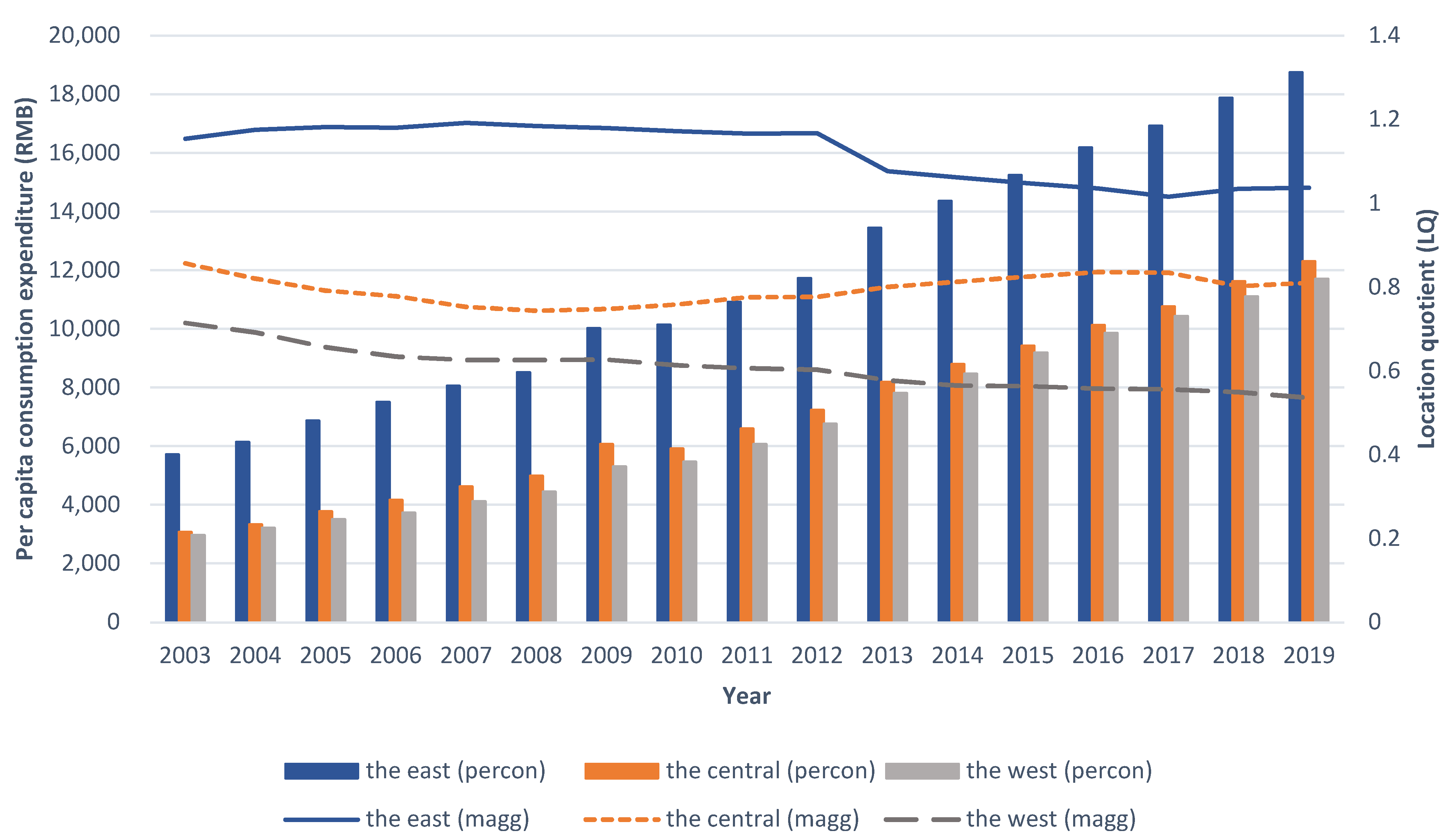
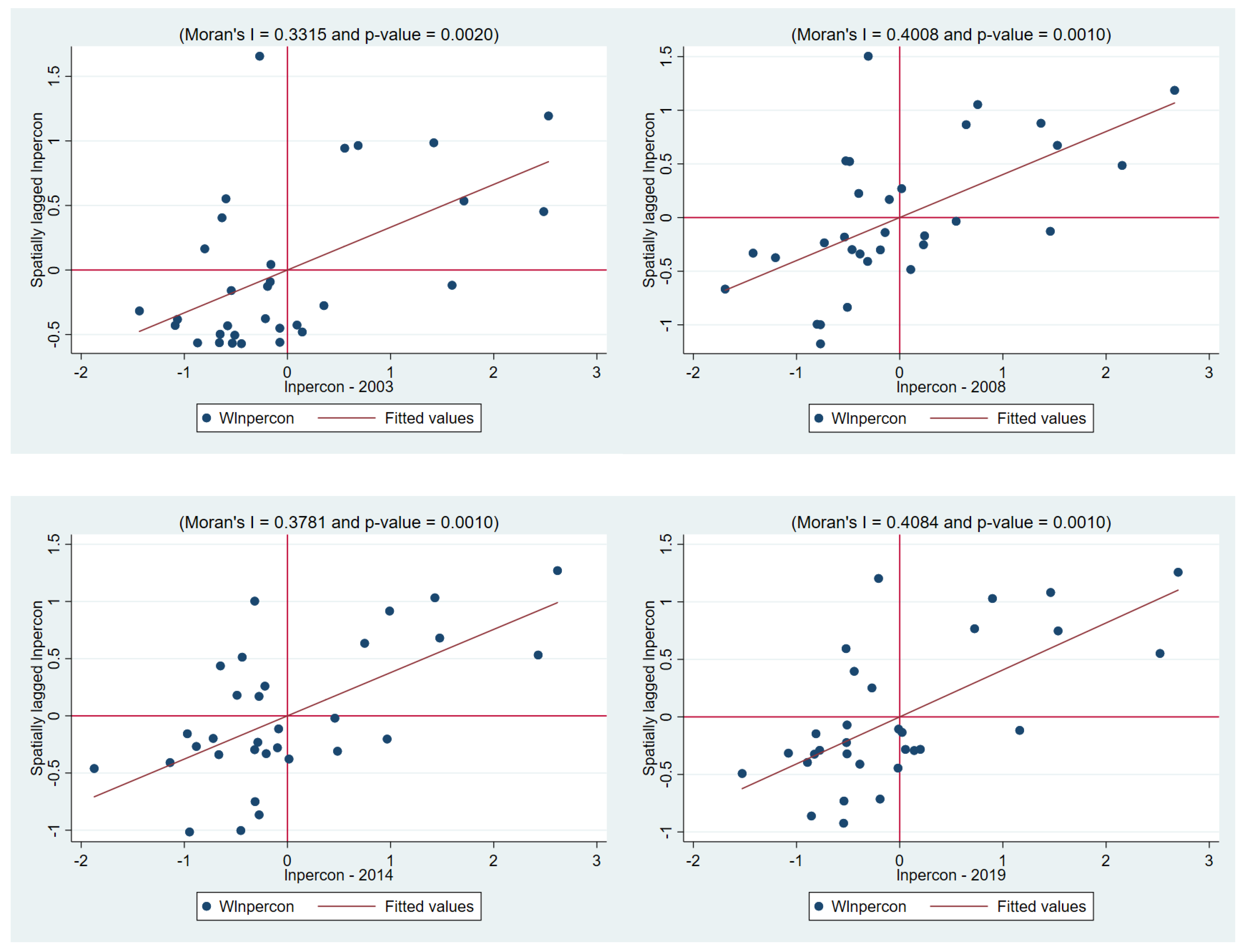
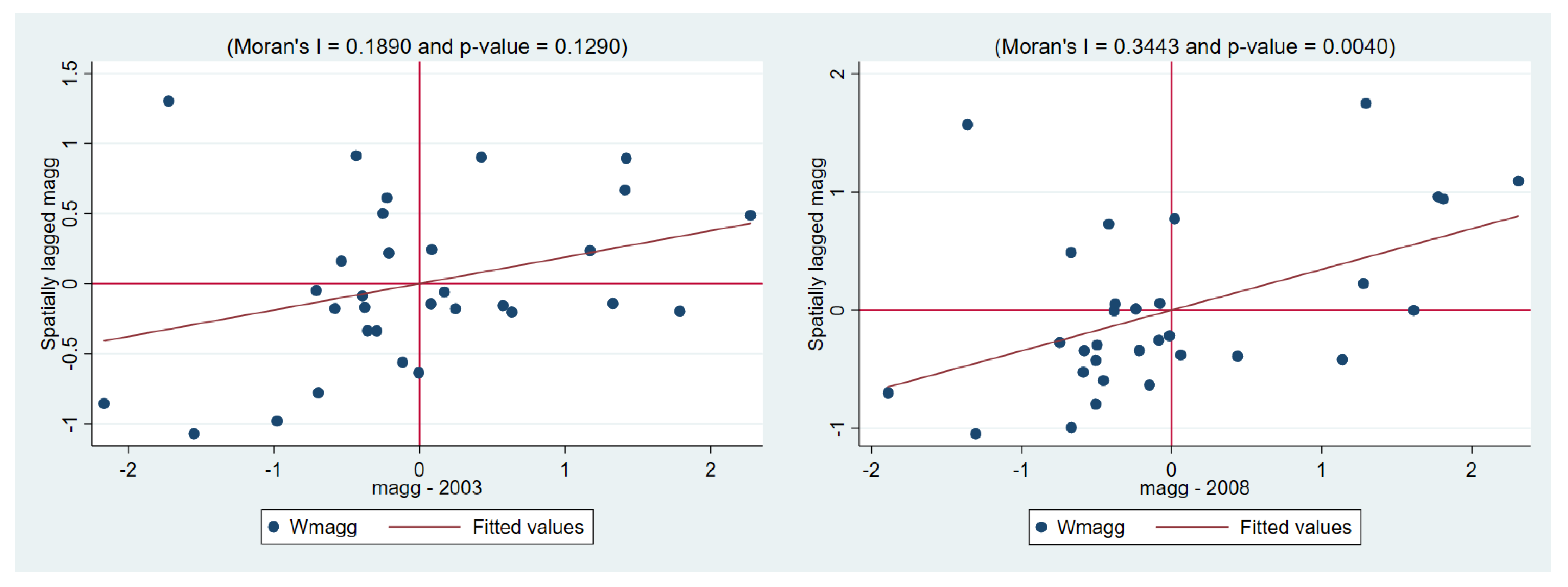
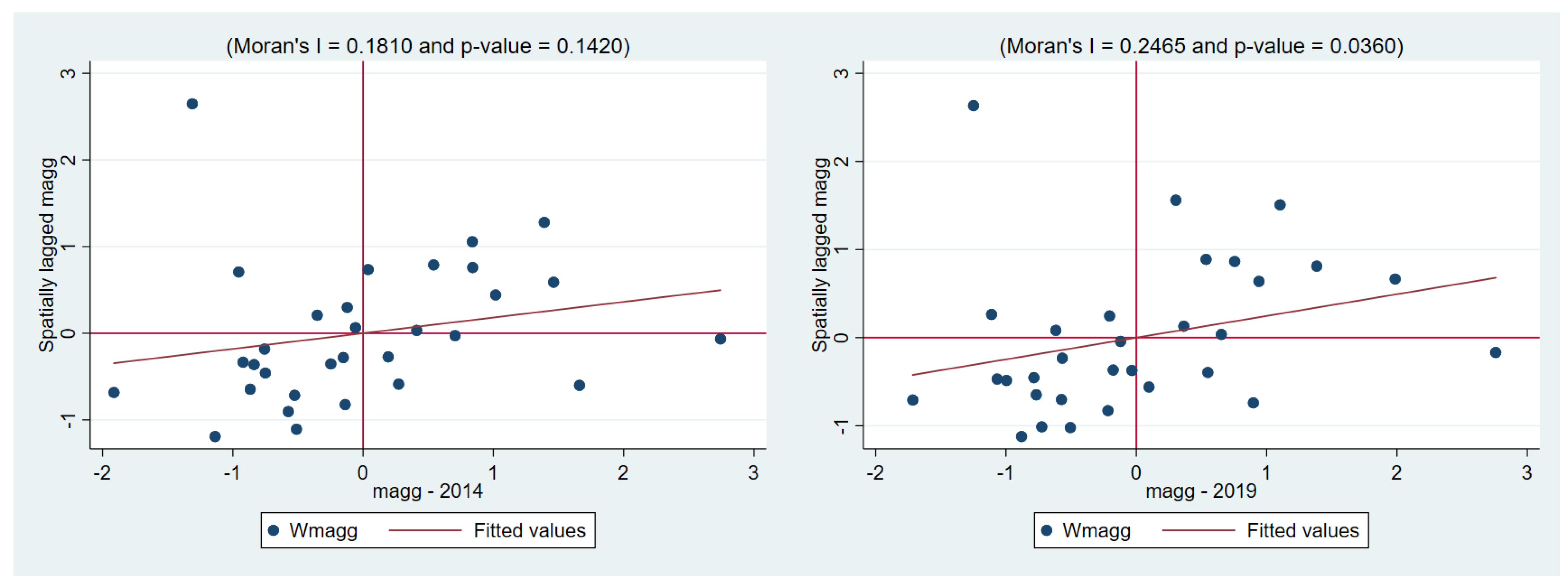
3.3. Spatial Correlation Analysis

Spatial econometric models should be adopted to analyze problems when there is spatial autocorrelation of observations. Helbich et al. [67] concluded that many scholars adopt Moran’s I index to test the spatial correlation of objects. There are two kinds of Moran’s I: the global spatial autocorrelation index and the local spatial autocorrelation index. The formula of the global spatial autocorrelation Moran’s I index is expressed as follows:
Global Moran s   I = n i = 1 n j = 1 n W i j   ×   i = 1 n j = 1 n W i j x i x ¯   x j x ¯ i = 1 n x i x ¯ 2
W i j = 1 ,   i f   p r o v i n c e   i   a n d   j   a r e   a d j a c e n t   0 ,   i f   n o t  
where n is the total number of provinces; W i j is the spatial matrix, which sets the weight matrix of 0 and 1 according to whether the space between the two regions is adjacent; x i and x j represent the observations in the ith province and jth province, respectively; x ¯ is the average of x i and x j . The value of Moran’s I is between −1 and 1. If the value is greater than 0, the correlation between samples is positive, which means that a positive spatial correlation exists in the variable. If the value is close to −1, the correlation between samples is negative, which indicates that the variable represents a negative spatial correlation. If the value is closer to 1, the agglomeration effect is stronger. On the other hand, the closer the value is to −1, the more intense the diffusion effect is. When the value is equal to 0, this illustrates no spatial relationship. This paper conducts global space-related tests of residents’ consumption and industrial agglomeration for 31 provinces in China from 2003 to 2019, analyzing the spatial interactions in residents’ consumption or industrial agglomeration between provinces. The results are given in Table 2.
Table 2 shows the results of the global Moran’s I index of residents’ consumption and industrial agglomeration in China from 2003 to 2019. The results show that the Moran’s I values of residents’ consumption are statistically significant at the 1% level and that the values are positive. The Moran’s I values of industrial agglomeration are also positive at a significance level of 5%, except in 2003, 2013, 2014, 2015, and 2016. The results show that, to a significant degree, China’s residents’ consumption between provinces is not completely random. A spatial autocorrelation of residents’ consumption exists, which means that larger values are adjacent to larger values and smaller values are adjacent to smaller values in China.
In the above global correlation analysis, the global Moran’s I is significant, especially for residents’ consumption. Therefore, residents’ consumption is spatially correlated among the Chinese provinces. However, where the spatial agglomeration phenomenon exists is still unknown. Thus, the local Moran’s I index is used to help further explain the results. The local Moran’s I index is used to test the cluster-localized situation between observations [68]. The formula for the local spatial autocorrelation Moran’s I index is as follows:
Local   Moran s   I = x i x ¯ S 2 j 1 n W i j x i x ¯
where a local Moran’s I > 0 shows that a smaller value is surrounded by other small values (small–small), or a larger value is surrounded by other large values (large–large). Moreover, Moran’s I < 0 indicates that a larger value is surrounded by small values (large–small), or a smaller value is surrounded by larger values (small–large).
This paper uses Moran scatterplots to further verify the spatial correlation between residents’ consumption and manufacturing industrial agglomeration. Figure 2 and Figure 3 present the Moran scatterplots of residents’ consumption and industrial agglomeration for 31 Chinese provinces in 2003, 2008, 2014, and 2019. The sample value of 31 provinces is not randomly distributed in four quadrants, but rather in a regular gathering distribution. Regarding the distribution of Moran scatterplots of residents’ consumption, there are 21 provinces located in the first and third quadrants in 2008 and 2014, 22 in 2019, and 23 in 2003, where people’s consumption is high and the surrounding provinces’ consumption is also high, such as in Beijing, Tianjin, and Shanghai, and those provinces with lower consumption have neighboring provinces with lower consumption, such as Guizhou, Gansu, and Xinjiang. In addition, provinces in the first and third quadrants account for about 70% of all provinces in these four years. For the independent variable of industrial agglomeration, the numbers of scattered points from 2003 to 2019 located in the first and third quadrants are 18, 21, 23, and 22 respectively. However, more scattered points in 2003 and 2008 tend towards 0, and the Moran’s I values of industrial agglomeration in recent years are relatively low. Thus, Figure 2 again confirms that significant spatial autocorrelation of residents’ consumption exists.

3.4. Model Specification

The initial OLS model is based on Song et al. [7] and Wu Peng et al. [62].
l n p e r c o n i t = α l i t + β 1 m a g g i t + β 2 m a g g i t 2 + δ C V i t + ε i t
where i and t represent the province and time period, respectively; the dependent variable l n p e r c o n i t is the logarithm of per capita consumption expenditure (lnpercon); l i t is a vector of constant terms; m a g g i t is manufacturing industrial agglomeration. The independent variables are m a g g i t and m a g g i t 2 . C V i t is a series of control variables, including lntech, lngdp, lnperinc, open, gov, stru, and lnurban [12,52,56,58,59,61]. α and β are the coefficients and ε i t is the error term.
This paper studies the industrial agglomeration that not only affects the consumption of residents in the region, but also the consumption of surrounding residents. Residents’ consumption between neighboring regions also has spatial correlation and spatial spillover effects. Therefore, this paper will adopt a spatial panel model, the spatial Durbin model (SDM), which can take into account the spatial dependence of the dependent variable and the independent variables at the same time. The SDM includes the static spatial Durbin model (SSDM) (Equation (6)) and the dynamic spatial Durbin model (DSDM) (Equation (7)). The spatial econometric model was first proposed by Cliff and Ord [69] and was initially aimed at cross-sectional data before being expanded into a panel model by Anselin [70], X. Chen [71], Elhorst and Fréret [72], Lee and Yu [73], and P. Zhao et al. [74]:
l n p e r c o n i t = ρ j = 1 n W i j l n p e r c o n j t + α l i t + β 1 m a g g i t + β 2 m a g g i t 2 + θ 1 j = 1 n W i j m a g g j t + δ   ×   C V i t + φ j = 1 n W i j C V j t + ε i t
l n p e r c o n i t = ρ j = 1 n W i j l n p e r c o n j t + η l n p e r c o n i , t 1 + π j = 1 n W i j l n p e r c o n j , t 1 + α l i t + β 1 m a g g i t + β 2 m a g g i t 2 + θ 1 j = 1 n W i j m a g g j t + δ   ×   C V i t + φ j = 1 n W i j C V j t + ε i t
where l n p e r c o n i , t 1 is the per capita consumption expenditure of the previous year and W i j is the spatial weight matrix, which sets the weight matrix of 0 and 1 according to whether the space between the two regions is adjacent. ρ, π, θ 1 , θ 2 , and φ are the spatial coefficients. For example, ρ j = 1 n W i j l n p e r c o n j t is the interactive relationship between the dependent variables in adjacent regions. If ρ > 0, there is a spatial spillover effect of the dependent variable in the neighboring area. If ρ < 0, there is a siphon effect in the neighboring area—that is, the region with greater economic strength and development potential attracts the superior resources from the neighboring region.
When choosing between a fixed-effect model and random-effect model, Ishak and Bani [75] stated that the Hausman test can be used to evaluate whether there is a systematic difference between the coefficients FE and RE. According to the Hausman test, the p-value in this paper is equal to 0.0000, which proves that the result is significant at a 1% level. Therefore, this paper chooses the fixed-effect model instead of a random-effect model. In addition, the correlation coefficient between lngdp and lnurban is 0.861 and that between lngdp and lnperinc is 0.961, which shows that the three variables have strong correlations and there is multicollinearity. Therefore, we use stepwise regression and the VIF (variance inflation factor) to eliminate redundant variables. The results show that lngdp and stru are redundant and should be deleted from the control variables. Thus, our proposed model is expressed as follows.
l n p e r c o n i t = ρ j = 1 n W i j l n p e r c o n j t + η l n p e r c o n i , t 1 + α l i t + β 1 m a g g i t + β 2 m a g g i t 2 + δ 1 l n t e c h i t + δ 2 l n p e r i n c i t + δ 3 o p e n i t + δ 4 g o v i t + δ 5 l n u r b a n i t + φ 1 j = 1 n W i j l n p e r i n c j t + φ 2 j = 1 n W i j l n t e c h j t + φ 3 j = 1 n W i j l n u r b a n j t + ε i t

4. Results and Discussion

4.1. Empirical Results

Based on the previous analysis, this article uses the fixed effects of the dynamic spatial Durbin model (DSDM) to analyze the impact of industrial agglomeration on residents’ consumption on the national level and in the eastern, central, and western regions. The dynamic spatial Durbin model (DSDM) is shown in Table 3. (I), (II), (III), and (IV) are the regression results at the national, eastern, central, and western levels, respectively. Their R 2 values are over 95%, indicating that the goodness of fit is good and that the models used in this paper have strong explanatory power. The spatial coefficients ρ of all regression results in Table 3 pass the test at a significance level of 1%, and the coefficients are significantly positive, indicating that the spatial econometric model estimation is effective and residents’ consumption in neighboring regions has a positive spillover impact on the region under study. Simultaneously, the results show that most of the coefficients of l n p e r c o n i , t 1 are significant at the 1% level, which verifies that the DSDM is better than the SSDM, which is consistent with the previous theory.
The values of the coefficients of the independent variables magg and m a g g 2 are significant at the 5% level on the national level and at the 1% level in the eastern region, but they are not significant in the central or western region. Therefore, regarding the impact of manufacturing industrial agglomeration on resident consumption, the empirical results show that manufacturing industrial agglomeration and residents’ consumption present an inverted “U-shaped” relationship, although the coefficients in different regions are a little different. As the degree of manufacturing industrial agglomeration increases, residents’ consumption will rise, and when it reaches a certain value, residents’ consumption will decrease as the degree of agglomeration increases. When industrial agglomeration is estimated to be about 1.01 in regression (I), the impact of industrial agglomeration on residents’ consumption reaches its maximum. Manufacturing industrial agglomerations in the central and west are lower than 1.01 from 2003 to 2019, as they were in the initial stage of industrial agglomeration. Thus, the effects of industrial agglomeration on residents’ consumption in the central and west are still positive. However, the level of industrial agglomeration in the east region is higher than the threshold value, and thus, agglomeration has an inhibitory effect on residents’ consumption.
As shown in Table 3, the signs of the control variables, including lnperinc, gov, and lnurban, in their effects on residents’ consumption are the same at the national level and the regional level, with only slight differences in the extent of their effects. The impacts of residents’ income, government expenditure scale, and urbanization rate on residents’ consumption are significantly positive at the 1% level and 5% level, indicating that these factors can promote an increase in residents’ consumption. Technological innovation in the east of China has a significantly positive effect on residents’ consumption at the 5% level, which is in line with the actual situation. However, in other regions, it is negative. The degree of openness is significantly negative at the 1% level in regression (I) and at the 10% level in regression (II), verifying that it has an inhibitory effect on residents’ consumption in these regions, but the value in the central region is positive, indicating that the degree of openness has a positive impact on residents’ consumption in the central region. Furthermore, Table 3 adds the spatial spillover effects of several variables, such as residents’ income and so on. The results show that the spatial spillover effects of residents’ income are significantly negative at the 1% level in all regions, suggesting that residents’ income in the surrounding provinces is unfavorable for residents’ consumption in a province. The spatial spillover effect of technological innovation in the center of China is negative at a significance level of 5%, which shows that technological innovation in the surrounding provinces inhibits residents’ consumption in the central region. The spatial spillover effect of urbanization rate is significantly negative at the 1% level in regression (I).

4.2. Robustness Test

This paper will conduct a robustness test from two perspectives: replacing independent variables and the spatial weight matrix. First, the robustness test is performed by selecting other indicators as explanatory variables, and the independent variable manufacturing industrial agglomeration (magg) is replaced with service industry agglomeration (sagg). In addition, some scholars believe that different spatial weight matrices can be constructed to verify whether the spatial model design is reasonable [76,77]. Thus, this paper introduces the geographic distance weight matrix (the geographic distance weight matrix: The main diagonal elements are 0; (i, j) of the non-main diagonal is w i j = 1/ d i j (i ≠ j), and d i j is the distance between area i and area j) to test its robustness. The results are shown in Table 4. Model A is the robustness estimation of the above DSDM model (I) from Table 3. Model B is the robustness estimation after replacing the independent variables. Model C is the robustness estimation after changing the spatial weight matrix using the geographic distance weight matrix. W * lnperinc, W * lntech, and W * lnurban are the spatial coefficients. The robustness estimation results of models A, B, and C show that all of the spatial coefficients ρ pass the test at the 1% significance level, indicating that the three spatial models are effective. Model B shows that the coefficient of sagg is significant at the 5% level and the signs of the coefficient of magg in model A and model C are the same, proving that the results are still robust.

4.3. Discussion

This study aimed to analyze the effects of manufacturing industrial agglomeration on residents’ consumption in China. Firstly, we found that residents’ consumption in different regions of China is not randomly distributed, but has a significant positive spatial correlation. This result is consistent with Song et al. [7]. In the past, most research on consumption, such as that of Alimi [53] and Kozyreva et al. [12], has paid little attention to its spatiality. However, in the present study, both Moran’s I and the spatial coefficient of residents’ consumption are positive, indicating that residents’ consumption in a certain province will be affected by that of neighboring provinces.
Secondly, manufacturing industrial agglomeration and residents’ consumption present an inverted U-shaped relationship. In the initial stage of manufacturing agglomeration, industrial agglomeration promotes residents’ consumption. However, when manufacturing industrial agglomeration reaches a certain level, industrial agglomeration may inhibit residents’ consumption. The results for the impact of industrial agglomeration on residents’ consumption are similar to those of Song et al. [7] and Wang [47], but are not consistent with those of Liu and Xu [51] and Wu et al. [62]. Regarding the initial stage, the most common explanation in the past has been that industrial agglomeration can increase residents’ consumption through a scale effect, as put forward by Norman and Venables [44] and Rosenthal [45]. Then, due to the crowding effect on the limited resources, as manufacturing industrial agglomeration exceeds a certain value, it will have a negative effect on residents’ consumption.
Additionally, based on Figure 1 and Table 3, we find that the unbalanced development of manufacturing industrial agglomeration in the east, center, and west of China exists and that the effects of industrial agglomeration on residents’ consumption vary across regions when keeping other variables fixed. Manufacturing industrial agglomeration in the eastern region has always been the highest. Manufacturing agglomeration in this region is relatively mature and exceeds the threshold, which means that it will have a certain inhibitory effect on residents’ consumption. However, the concentration of manufacturing industries in the central and western regions still has a positive effect on residents’ consumption because their values of industrial agglomeration are lower than the threshold.
Fourthly, according to the results of the control variables, residents’ income, government expenditure scale, and urbanization rate have significantly positive effects on residents’ consumption, showing that these three factors can be beneficial for the improvement of residents’ consumption. These results are in line with those of Alimi [53], Shi and Nie [54], Rakhmanov [56], and Cao and Xu [58]. Furthermore, residents’ income, technological innovation, and urbanization rate have negative spatial spillover effects on residents’ consumption at a 1% significance level, indicating that residents’ income, technological innovation, and urbanization rate in neighboring provinces are not conducive to residents’ consumption. One likely reason for this is that if the income level, technological innovation, and urbanization of the two neighboring regions are quite different, the consumption level and standards of living in the developed region will be better than those of the developing region, which may attract the residents of the developing region to the developed region. To a certain extent, this will dampen consumption in the developing region. Therefore, the balanced development of each region is very important.

5. Conclusions

In the post-epidemic era, residents’ consumption has played a pivotal role in stimulating China’s economy. The governments of various regions in China continue to encourage and stimulate consumer consumption. Among them, the deployment of industrial agglomeration is critical. This paper examines the regional characteristics of Chinese residents’ consumption and industrial agglomeration from a spatial perspective and measures their spatial relationship. Based on the analysis of the theoretical mechanism of the impact of manufacturing industrial agglomeration on residents’ consumption, using data from 31 provinces in China from 2003 to 2019, the impact of manufacturing industrial agglomeration on residents’ consumption has been verified and discussed. The following suggestions and limitations can be drawn.
First, when attempting to stimulate resident consumption, local governments should consider the connection between the local area and neighboring provinces and increase the consumption of residents between regions. This is conducive not only to increasing local residents’ consumption, but also to increasing residents’ consumption in other regions so as to achieve a win–win effect. Second, the Chinese government can transfer some of the manufacturing agglomeration in the eastern regions to central and western areas to encourage provinces in the two regions to actively cultivate and develop agglomerations of manufacturing industries. The eastern region should strive to improve the quality and efficiency of their manufacturing agglomeration to prevent a congestion effect of manufacturing agglomeration due to excessive and low-end agglomeration. Third, all regions should continue to promote urbanization, improve residents’ income, and increase the government expenditure scale in order to promote an increase in residents’ consumption. Fourth, the Chinese government should work to reduce residents’ income gaps and unbalanced technological innovation and urbanization between regions. Otherwise, increasing residents’ income, technological innovation, and urbanization in surrounding areas will inhibit the increase in residents’ consumption in a local area.
The findings of this study could be used to evaluate the effects of manufacturing industrial agglomeration on residents’ consumption in other developing countries, such as Vietnam. However, this study has its limitations. First, we do not consider other methods to calculate the degree of industrial agglomeration, such as the spatial Gini coefficient, which could have different influences on residents’ consumption. In addition, this study uses a spatial adjacency matrix and a geographic distance weight matrix in the specified model. Hence, future research on spatial weight matrixes may want to focus on the economic distance weight matrix (the economic distance weight matrix: The main diagonal elements are 0; (i, j) of the non-main diagonal is W i j = 1 Y ¯ i Y ¯ j (ij), Y ¯ i is the average real GDP per capita of region i in the sample from 2003 to 2017, and Y ¯ j is the average real GDP per capita of region j in the sample), which could better fit the development of a regional economy.

Author Contributions

S.Z. proposed the research framework and drafted and finalized the paper. Y.B., A.I.S. and J.A.G. worked on the review and editing. All authors have read and agreed to the published version of the manuscript.

Funding

This research received no external funding.

Institutional Review Board Statement

Not applicable.

Informed Consent Statement

Not applicable.

Data Availability Statement

The data used to support the findings of this study are included within the text.

Acknowledgments

The authors would like to thank Caroline and Gerry for their language assistance and the anonymous reviewers for their constructive comments.

Conflicts of Interest

The authors declare no conflict of interest.

References

  1. Ali, M.; Alam, N.; Rizvi, S.A.R. Coronavirus (COVID-19)—An epidemic or pandemic for financial markets. J. Behav. Exp. Financ. 2020, 27, 100341. [Google Scholar] [CrossRef] [PubMed]
  2. Haroon, O.; Rizvi, S.A.R. COVID-19: Media coverage and financial markets behavior—A sectoral inquiry. J. Behav. Exp. Financ. 2020, 27, 100343. [Google Scholar] [CrossRef] [PubMed]
  3. Narayan, P.K. Oil price news and COVID-19—Is there any connection? Energy Res. Lett. 2020, 1, 13176. [Google Scholar] [CrossRef]
  4. Han, H.; Si, F. How does the composition of asset portfolios affect household consumption: Evidence from China based on micro data. Sustainability 2020, 12, 2946. [Google Scholar] [CrossRef] [Green Version]
  5. Li, J.; Wu, Y.; Xiao, J.J. The impact of digital finance on household consumption: Evidence from China. Econ. Model. 2020, 86, 317–326. [Google Scholar] [CrossRef] [Green Version]
  6. Li, L.; Zhu, Y. The impact of China’s urbanization level on household consumption. Rev. Cercet. Interv. Soc. 2021, 72, 378–397. [Google Scholar] [CrossRef]
  7. Song, F.; Sun, Y.; Song, B. Research on the impact of industrial agglomeration on urban and rural residents’ consumption—Based on the dynamic spatial panel model. Mod. Financ. J. Tianjin Univ. Financ. Econ. 2020, 5, 74–84. [Google Scholar]
  8. Chang, Y.; Wu, P. Analysis of the influence mechanism and effect difference of industrial agglomeration on income distribution. Collection 2018, 9, 66–78. [Google Scholar]
  9. Su, D.; Sheng, B.; Shao, Z. Industrial agglomeration and quality upgrade of enterprise export products. China Ind. Econ. 2018, 11, 117–135. [Google Scholar]
  10. Zhang, K. The impact of different industrial agglomerations on regional innovation and its spatial spillover effects. J. Xi’an Jiaotong Univ. 2019, 2, 12–19. [Google Scholar]
  11. Zhao, H. An Interregional Comparative Study on the Short-sighted Consumption Behavior of Chinese Urban Residents. Bus. Econ. Res. 2016, 6, 120–122. [Google Scholar]
  12. Kozyreva, P.M.; Di, Z.; Nizamova, A.E.; Smirnov, A.I. Justice and inequality in the household consumption in Russia and China: A comparative analysis. Bulletin of the Peoples’ Friendship University of Russia. Ser. Sociol. 2021, 21, 50–66. [Google Scholar]
  13. Liu, W. Research on the spatial effects of provincial urban residents’ consumption: Based on the spatial panel data model. Contemp. Econ. 2017, 9, 140–142. [Google Scholar]
  14. Yang, J.; Luo, S.; Wang, J. Spatial econometric analysis of rural residents’ consumption from the perspective of double uncertainty. J. Huazhong Agric. Univ. 2018, 5, 94–102. [Google Scholar]
  15. Marshall, A. Principles of Economics: Unabridged, 8th ed.; Cosimo. Inc: New York, NY, USA, 1980. [Google Scholar]
  16. Weber, A. Theory of the Location of Industries; The University of Chicago Press: Chicago, IL, USA, 1929. [Google Scholar]
  17. Porter, M.E. The competitive advantage of nations. Compet. Intell. Rev. 1990, 1, 14. [Google Scholar] [CrossRef]
  18. Krugman, P. Increasing returns and economic geography. J. Polit. Econ. 1991, 99, 483–499. [Google Scholar] [CrossRef]
  19. He, Q.; Zhang, Z. Exploration on the Distribution of Economic Activity: Technology Spillover. Environmental Pollution and Trade Liberalization. Sci. Geogr. Sin. 2015, 35, 161–167. [Google Scholar]
  20. Hu, S.; Song, W.; Li, C.; Zhang, C.H. The evolution of industrial agglomerations and specialization in the Yangtze River Delta from 1990–2018: An analysis based on firm-level big data. Sustainability 2019, 11, 5811. [Google Scholar] [CrossRef] [Green Version]
  21. Lu, Y.; Cao, K. Spatial analysis of big data industrial agglomeration and development in China. Sustainability 2019, 11, 1783. [Google Scholar] [CrossRef] [Green Version]
  22. Zhang, L.; Rong, P.; Qin, Y.; Ji, Y. Does industrial agglomeration mitigate fossil CO2 emissions? An empirical study with spatial panel regression model. Energy Procedia 2018, 152, 731–737. [Google Scholar] [CrossRef]
  23. Feng, D.; Li, J.; Li, X.; Zhang, Z. The effects of urban sprawl and industrial agglomeration on environmental efficiency: Evidence from the Beijing–Tianjin–Hebei Urban Agglomeration. Sustainability 2019, 11, 3042. [Google Scholar] [CrossRef] [Green Version]
  24. Lei, Y.; Zheng, M.; Sun, J. The impact of industrial agglomeration on haze pollution of key urban agglomerations in China. Soft Sci. 2020, 34, 64–69. [Google Scholar]
  25. Zhang, G.; Chen, C. Research on dynamic relationship between industrial agglomeration and urban eco-efficiency. Sci. Technol. Prog. Countermeas. 2019, 36, 48–57. [Google Scholar]
  26. Guo, Y.; Tong, L.; Mei, L. The effect of industrial agglomeration on green development efficiency in Northeast China since the revitalization. J. Clean. Prod. 2020, 258, 120584. [Google Scholar] [CrossRef]
  27. Wang, Y.; Wang, J. Does industrial agglomeration facilitate environmental performance: New evidence from urban China? J. Environ. Manag. 2019, 248, 109244. [Google Scholar] [CrossRef]
  28. Zhao, H.; Cao, X.; Ma, T. A spatial econometric empirical research on the impact of industrial agglomeration on haze pollution in China. Air Quality. Air Qual. Atmos. Health 2020, 13, 1–8. [Google Scholar] [CrossRef]
  29. Jacobs, J. The Economy of Cities; Vintage: New York, NY, USA, 1961. [Google Scholar]
  30. Wu, S.; Li, S. The relationship between specialization, diversification and industrial growth: An empirical study based on China’s provincial manufacturing panel data. Dr. Diss. 2011, 8, 21–34. [Google Scholar]
  31. Zhu, H.; Dai, Z.; Jiang, Z. Industrial agglomeration externalities, city size, and regional economic development: Empirical research based on dynamic panel data of 283 cities and GMM method. Chin. Geogr. Sci. 2017, 27, 456–470. [Google Scholar] [CrossRef] [Green Version]
  32. Sullivan, A.O. Urban Economics; McGraw-Hill Education: New York, NY, USA, 2007. [Google Scholar]
  33. Chen, J.; Chen, H. A review of agglomeration measurement methods: Research based on frontier literature. J. Southwest Univ. Natl. 2017, 4, 134–142. [Google Scholar]
  34. Fang, Z. The spatial agglomeration characteristics and influencing factors of Guangzhou convention and exhibition enterprises. Acta Geogr. Sin. 2013, 68, 464–476. [Google Scholar]
  35. Liao, X.; Qiu, D.; Lin, Y. Research on the Spatial Agglomeration Measurement Theory and Countermeasures of China’s Science and Technology Service Industry Based on Location Entropy. Res. Sci. Technol. Manag. 2018, 2, 171–178. [Google Scholar]
  36. Wei, P.; Yang, Z.; Li, J.; Fang, L. Research on the measurement of manufacturing agglomeration in domestic channels of the second eurasian continental bridge. Sci. Technol. Prog. Countermeas. 2017, 8, 58–65. [Google Scholar]
  37. Peters, D.J. Revisiting industry cluster theory and method for use in public policy: An example of identifying supplier-based clusters in Missouri. J. Reg. Anal. Policy 2004, 34, 107–133. [Google Scholar]
  38. Jiang, Y.; Xu, X. Analysis of the agglomeration level and efficiency measurement of forestry industry in Heilongjiang Province. For. Econ. 2016, 38, 55–58. [Google Scholar]
  39. Zhang, Q.; Guo, S.; Huang, Z. Research on the measurement of the impact of industrial agglomeration on the efficiency of industrial technology innovation. Sci. Manag. Res. 2016, 3, 60–63. [Google Scholar]
  40. Behrens, K.; Gaigné, C.; Thisse, J.-F. Industry location and welfare when transport costs are endogenous. J. Urban Econ. 2008, 65, 195–208. [Google Scholar] [CrossRef]
  41. Ji, S.; Zhu, Y.; Zhang, X. Research on the improvement effect of industrial agglomeration on resource mismatch. China Ind. Econ. 2016, 6, 73–90. [Google Scholar]
  42. Yuan, H.; Liu, Y.; Hu, S.; Feng, Y. Does industrial agglomeration exacerbate environmental pollution?—Based on the perspective of foreign direct investment. Resour. Environ. Yangtze River Basin 2019, 28, 794–804. [Google Scholar]
  43. Fujita, M.; Thisse, J.-F. Does geographical agglomeration foster economic growth? And who gains and loses from it? Jpn. Econ. Rev. 2003, 54, 121–145. [Google Scholar] [CrossRef]
  44. Norman, V.D.; Venables, A.J. Industrial agglomerations: Equilibrium, welfare and policy. Economica 2004, 71, 543–558. [Google Scholar] [CrossRef] [Green Version]
  45. Rosenthal, S.S. Chapter 49 Evidence on the nature and sources of agglomeration economies. Handb. Reg. Urban Econ. 2004, 4, 2119–2171. [Google Scholar]
  46. Xiao, L.; Hong, Y. Financial agglomeration, regional heterogeneity and resident consumption: An empirical analysis based on dynamic panel model. Soft Sci. 2017, 31, 29–37. [Google Scholar]
  47. Wang, C. Research on the impact mechanism of the coordinated development of industrial agglomeration on consumption upgrading. Bus. Times 2020, 5, 189–192. [Google Scholar]
  48. Wu, Y.; Pu, Y. Welfare effect and policy research of regional excessive agglomeration negative externality: Simulation Analysis Based on Spatial Economics. J. Financ. Econ. 2008, 34, 106–115. [Google Scholar]
  49. Liu, X.; Yin, X. Spatial externalities and regional wage differences: A dynamic panel data study. China Econ. Q. 2008, 8, 77–98. [Google Scholar]
  50. Wang, H.; Chen, Y. Research on the industrial agglomeration effect and regional wage disparity. Econ. Rev. 2010, 5, 72–81. [Google Scholar]
  51. Liu, J.; Xu, K. Does industrial agglomeration affect the welfare of regional residents? Explor. Econ. 2016, 6, 72–79. [Google Scholar]
  52. Wu, Y.; Pan, H. Research on the spatial spillover effect of total factor productivity on resident consumption. Theory Pract. Financ. Econ. 2020, 41, 126–131. [Google Scholar]
  53. Alimi, R.S. Keynes’ Absolute Income Hypothesis and Kuznets Paradox; Munich Personal RePEc Archive: Munich, Germany, 2013. [Google Scholar]
  54. Kai, S.; Li, N. The impact of urbanization on the consumption of urban and rural residents. Urban Issues 2014, 6, 87–93. [Google Scholar]
  55. Deng, G.; Li, X.; Zhang, Z. Research on the Impact of Government Expenditure on Resident Consumption—Based on the Analysis of the Spatial Dynamic Panel Model. Collect. Essays Financ. Econ. 2016, 208, 19–28. [Google Scholar]
  56. Rakhmanov, F. Issues of improving social policy in the republic of Azerbaijan. Sci. News Azerbaijan State Econ. Univ. 2017, 5, 32–41. [Google Scholar]
  57. Xiaojia, L.; Cheng, J.; Laoer, W. Research on the spatial effect of local fiscal expenditure on household consumption. World Econ. Collect. 2016, 1, 108–120. [Google Scholar]
  58. Cao, J.; Xu, P. Government fiscal expenditure, opening to the outside world and changes in household consumption structure: Empirical evidence from China’s experience. Bus. Econ. Res. 2019, 23, 166–168. [Google Scholar]
  59. Longpeng, T. Analysis of housing prices, residents’ income level and consumption upgrade based on panel quantile regression analysis. Consum. Econ. 2019, 35, 61–69. [Google Scholar]
  60. Zhongjie, Z.; Xue, L. An empirical study on the impact of China’s urbanization on resident consumption. Stat. Decis. Mak. 2019, 8, 126–130. [Google Scholar]
  61. Caihong, H.; Xiaoqing, Z. Driven by innovation, space spillover and consumer demand. Explor. Econ. Issues 2020, 2, 11–20. [Google Scholar]
  62. Peng, W.; Yuan, C.; Huaizhong, M. Research on the economic welfare effect of industrial agglomeration—Based on the perspective of resident welfare maximization. China Econ. Issues 2020, 3, 19–29. [Google Scholar]
  63. Chen, J.; Liu, Y.; Zou, M. The improvement of urban production efficiency under industrial collaborative agglomeration: Based on the background of integrated innovation and development power conversion. J. Zhejiang Univ. 2016, 1, 150–163. [Google Scholar]
  64. Dou, J.; Liu, Y. Can the collaborative agglomeration of the producer service industry and the manufacturing industry promote economic growth? Based on panel data of 285 prefecture-level cities in China. Mod. Financ. J. Tianjin Univ. Financ. Econ. 2016, 4, 92–102. [Google Scholar]
  65. Zhang, H.; Han, A.; Yang, Q. Analysis of the spatial effect of the collaborative agglomeration of China’s manufacturing and producer service industries. Quant. Techol. Econ. Res. 2017, 34, 3–20. [Google Scholar]
  66. Liu, T.; Pan, B.; Yin, Z. Pandemic, mobile payment, and household consumption: Micro-evidence from China. Emerg. Mark. Financ. Trade 2020, 56, 2378–2389. [Google Scholar] [CrossRef]
  67. Helbich, M.; Brunauer, W.; Vaz, E.; Nijkamp, P. Spatial heterogeneity in hedonic house price models: The case of Austria. Urban Stud. 2014, 51, 390–411. [Google Scholar] [CrossRef] [Green Version]
  68. Yang, X.; Wu, Y.; Shen, Q.; Dang, H. Measuring the degree of speculation in the residential housing market: A spatial econometric model and its application in China. Habitat Int. 2017, 67, 96–104. [Google Scholar] [CrossRef] [Green Version]
  69. Cliff, A.D.; Ord, K. Spatial autocorrelation: A review of existing and new measures with applications. Econ. Geogr. 2016, 46, 269–292. [Google Scholar] [CrossRef]
  70. Anselin, L. Some robust approaches to testing and estimation in spatial econometrics. Reg. Urban Econ. 1990, 20, 141–163. [Google Scholar] [CrossRef]
  71. Chen, X. Do “aging” and “fewer births” affect rural residents’ consumption?—An empirical study based on static and dynamic spatial panel models. J. Beijing Technol. Bus. Univ. 2015, 3, 118–126. [Google Scholar]
  72. Elhorst, J.P.; Fréret, S. Evidence of political yardstick competition in France using a two-regime spatial Durbin model with fixed effects. J. Reg. Sci. 2009, 49, 931–951. [Google Scholar] [CrossRef]
  73. Lee, L.F.; Yu, J. Efficient GMM estimation of spatial dynamic panel data models with fixed effects. J. Econom. 2014, 180, 174–197. [Google Scholar] [CrossRef]
  74. Zhao, P.; Zeng, L.; Lu, H.; Zhou, Y.; Hu, H.; Wei, X. Green economic efficiency and its influencing factors in China from 2008 to 2017: Based on the super-SBM model with undesirable outputs and spatial Durbin model. Sci. Total Environ. 2020, 741, 140026. [Google Scholar] [CrossRef]
  75. Ishak, S.; Bani, Y. Determinants of Crime in Malaysia: Evidence from Developed States. Int. J. Econ. Manag. 2017, 11, 607–622. [Google Scholar]
  76. Li, J.; Tan, Q.; Bai, J. Spatial measurement analysis of China’s regional innovative production energy: An empirical study based on static and dynamic spatial panel models. Manag. World 2010, 7, 43–55. [Google Scholar]
  77. Wang, Y.; Yang, X.; Zhang, W. Research on the Impact of Agricultural Insurance Development on Rural Total Factor Productivity: An Empirical Analysis Based on Spatial Econometric Models. J. Huazhong Agric. Univ. Soc. Sci. Ed. 2019, 6, 70–77. [Google Scholar]
Figure 1. The trends of per capita consumption expenditure (percon) and manufacturing industrial agglomeration (magg) in the east, center, and west of China from 2003 to 2019. Source: China Statistical Yearbook from 2004 to 2020. Note: The Renminbi (RMB) is the legal tender of China.
Sustainability 14 04364 g001
Figure 2. Moran scatterplots of residents’ consumption in 2003, 2008, 2014, and 2019.
Sustainability 14 04364 g002
Figure 3. Moran scatterplots of manufacturing industrial agglomeration in 2003, 2008, 2014, and 2019.
Sustainability 14 04364 g003aSustainability 14 04364 g003b
Table 1. Data used in this study.
VariableDescriptionSource
lnperconLogarithm of per capita consumption expenditureCSY
maggDegree of manufacturing industrial agglomerationCSY
lntechLogarithm of technological innovationCSY
lngdpLogarithm of regional economic development levelCSY
lnperincLogarithm of per capita incomeCSY
openDegree of opennessCSY
govGovernment expenditure scaleCSY
struIndustrial structureCSY
lnurbanLogarithm of urbanization rateCPESY
Note: CSY and CPESY represent the China Statistical Yearbook and China Population and Employment Statistics Yearbook, respectively.
Table 2. Global Moran’s I for residents’ consumption and industrial agglomeration.
YearsResidents’ ConsumptionIndustrial Agglomeration
Moran’s Ip-ValueMoran’s Ip-Value
20030.3310.0020.1890.060
20040.3230.0020.2330.023
20050.3630.0010.2700.010
20060.4020.0000.2880.006
20070.4040.0000.3410.002
20080.4010.0000.3440.001
20090.4510.0000.3120.004
20100.3800.0000.3180.003
20110.3830.0000.2900.007
20120.3550.0010.3080.004
20130.3740.0000.1920.055
20140.3780.0000.1810.068
20150.3810.0000.1790.070
20160.3700.0010.1940.053
20170.3820.0000.2220.030
20180.3970.0000.2350.022
20190.4080.0000.2470.017
Table 3. The dynamic spatial Durbin model (DSDM) regression results.
lnpercon(I)(II)(III)(IV)
L.lnpercon0.337 ***0.384 ***0.159 ***0.406 ***
(9.13)(5.45)(3.42)(4.12)
magg0.0827 **0.374 ***0.05010.317
(2.04)(3.83)(0.30)(0.92)
m a g g 2 −0.0411 **−0.146 ***−0.0312−0.201
(−2.57)(−3.98)(−0.32)(−0.74)
lntech−0.001110.0222 **−0.0252 ***−0.00472
(−0.15)(2.05)(−2.77)(−0.30)
lnperinc0.486 ***0.574 ***0.930 ***0.595 ***
(7.87)(5.14)(12.22)(3.45)
open−0.0643 ***−0.0511 *0.0931−0.110
(−3.92)(−1.72)(0.98)(−0.85)
gov0.149 ***0.458 ***0.1150.206 ***
(3.51)(4.01)(0.64)(3.36)
lnurban0.375 *** 0.09510.285 **
(5.76) (1.00)(2.27)
ρ0.536 ***0.432 ***0.501 ***0.386 ***
(14.53)(12.37)(22.34)(5.43)
W * lnperinc−0.327 ***−0.511 ***−0.528 ***−0.507 ***
(−5.93)(−10.47)(−5.97)(−3.60)
W * lntech−0.0158 −0.0267 **
(−1.53) (−2.35)
W * lnurban−0.470 ***
(−4.39)
R 2 0.9730.9840.9780.984
Note: t statistics in parentheses. *** p < 0.01, ** p < 0.05, * p < 0.1.
Table 4. Robustness test of the dynamic spatial Durbin model.
lnperconABC
L.lnpercon0.337 ***0.339 ***0.476 ***
(9.13)(8.95)(12.15)
magg0.0827 ** 0.0994 **
(2.04) (2.28)
m a g g 2 −0.0411 ** −0.0475 ***
(−2.57) (−2.86)
sagg 0.0462 **
(2.16)
lntech−0.001110.000019−0.00626
(−0.15)(0.00)(−0.84)
lnperinc0.486 ***0.475 ***0.403 ***
(7.87)(8.25)(5.39)
open−0.0643 ***−0.0666 ***−0.0573 ***
(−3.92)(−4.61)(−2.76)
gov0.149 ***0.168 ***0.222 ***
(3.51)(4.02)(3.98)
lnurban0.375 ***0.406 ***0.267 ***
(5.76)(6.21)(3.98)
ρ0.536 ***0.522 ***0.959 ***
(14.53)(14.24)(20.33)
W * lnperinc−0.327 ***−0.324 ***−0.809 ***
(−5.93)(−6.65)(−6.88)
W * lntech−0.0158−0.0130−0.0128
(−1.53)(−1.25)(−0.69)
W * lnurban−0.470 ***−0.473 ***−0.267
(−4.39)(−4.63)(−0.92)
R 2 0.9730.9720.738
Note: t statistics in parentheses. *** p < 0.01, ** p < 0.05, * p < 0.1.
Publisher’s Note: MDPI stays neutral with regard to jurisdictional claims in published maps and institutional affiliations.

