Article

Probabilistic Stability Evaluation Based on Confidence Interval in Distribution Systems with Inverter-Based Distributed Generations

1
Korea Smart Grid Association, Seoul 05638, Korea
2
School of Electrical Engineering, Korea University, Seoul 02841, Korea
3
Korea Electric Power Research Institute, Daejeon 34056, Korea
*
Author to whom correspondence should be addressed.
Sustainability 2022, 14(7), 3806; https://doi.org/10.3390/su14073806
Submission received: 16 February 2022 / Revised: 17 March 2022 / Accepted: 21 March 2022 / Published: 23 March 2022

Abstract

:
This study proposed a probabilistic methodology based on a confidence interval with the aim of overcoming the limitations of deterministic methods. A stability evaluation technique was required because the output variability of renewable energy can lead to instability of the distribution system. The proposed method can predict the possibility of violating stability in the future. It can also provide a theoretical basis for securing distribution system stability and improving operational efficiency by assessing the in-stability risk and worst-case scenarios. Because of steady-state analysis in the distribution system to which solar power is connected, the probability of violating the standard voltage during the daytime when PV fluctuations are severe was the highest. Moreover, as a result of a simulation of a three-phase short-circuit in the distribution system that is connected to the PV and WT, it was observed that it could violate the allowable capacity of the CB owing to the effects of the power demand pattern and output variability.

1. Introduction

To study the impact of renewable energy on power systems, it is necessary to provide a renewable energy output scenario by considering the output characteristics of each power source and applying an accurate prediction technique. The deterministic prediction methods based on machine learning and probabilistic prediction methods based on confidence intervals can be reviewed as prediction techniques. Although the stability of the system can be evaluated through deterministic prediction methods, the accuracy of the prediction cannot always be guaranteed. Thus, it may not be possible to accurately analyze the possibility of actual stability violations. Therefore, it is necessary to consider various output scenarios and evaluate the stability against the worst-case scenario by applying probabilistic prediction methods. Therefore, this study provided a probabilistic methodology that considers various RES outputs for distribution systems with inverter-based DGs.
According to the worldwide energy conversion policy, the interconnection of inverter-based distributed generation (DG) is increasing. However, renewable energy has problems with output variability and uncertainty, which can lead to instability of the distribution system or intensify difficulties in its operation. Unlike conventional power sources, the inverter-based DGs have no rotational inertia; thus, it is difficult to maintain the voltage and frequency of the AC power system [1]. Particularly, the output variability and uncertainty of renewable energy sources (RES) are factors that negatively affect the stability of distribution systems [2]. Recently, the number of renewable energy curtailments due to output fluctuations has rapidly increased, and as the interconnection rate of inverter-based DG increases, the duck curve deepens because of a sharp decrease in net load during the daytime [3]. Moreover, the existing power distribution system has a one-way power flow owing to the radial structure; however, DGs have been mainly connected to the end of the line, resulting in bidirectional power flow. Consequently, the method of protection cooperation and voltage distribution differs from those of the existing system [4]. To overcome these problems, studies on stability analysis technology in the distribution systems of interconnected RESs have been actively conducted worldwide. Riaz et al. [5] proposed a stochastic optimization in smart power systems to deal with the RES uncertainties wherein deterministic approaches are used to represent specific scenarios. A. Qamar et al. [6] presented a configuration detection model of ground grid to tackle the uncertainties and consider various grid configurations that continuously change according to the extension in a substation.
Studies on voltage stability evaluation and fault analysis methodology have been conducted to evaluate the stability of the next-generation power distribution systems. Voltage stability refers to the ability of the power system to allow the bus voltage to maintain the voltages of all bus lines within the allowable voltage range after a disturbance occurs from the initial operating conditions [7]. When the voltage of the system is unstable, the power system can experience a power outage or voltage collapse. Therefore, it is necessary to improve the efficiency of a power system by evaluating its voltage stability. Furthermore, fault analysis refers to the calculation of the fault current or voltage flowing through each bus or fault point in the event of a fault in the power system. Inaccurate fault current calculation may degrade system reliability and increase physical loss such as the replacement of protective devices; therefore, an efficient fault current calculation method considering renewable energy characteristics is required [8].
A traditional method for evaluating voltage stability is power flow calculation using the Newton–Raphson method. However, mathematical singularity problems occur at the voltage collapse point and a solution cannot be obtained. To solve this problem, a continuous power flow (CPF) method can be used to determine the approximate point of voltage collapse in the system [9,10]. This algorithm has strong convergence characteristics; however, the computational time and convergence characteristics are significantly influenced by the step size. An optimal power flow (OPF) can be performed to solve this problem. This method can simply and accurately solve the problem of the voltage collapse point of the Newton–Raphson power flow and the computational speed problem of the CPF method [11]. However, because these methods are based on mathematical formulas, there are limitations owing to time complexity.
Recently, simulation-based probabilistic techniques such as Monte Carlo simulation showed rapid and accurate voltage stability evaluation [12]. The probabilistic voltage stability can be analyzed based on the normal and cumulative distribution functions for the bus voltage that is derived by applying various output scenarios [13]. The author of [14] proposed a global sensitivity analysis methodology that considered RES variabilities and identified specific variables that affect the variability of the load margins. The author of [15] proposed a sequential Monte Carlo simulation to consider dynamic security assessment wherein acceleration methods are applied to improve the computational efficiency.
The authors of [16] computed the confidence interval and analyzed the probabilistic stability in distribution systems with inverter-based DGs. In [17], six types of Monte Carlo sampling techniques were presented for various RES output scenarios. Additionally, the scenario-based voltage stability was evaluated by calculating 95 and 99% confidence intervals; errors were compared using R2 and RMSE according to the sampling technique. The authors of [18] proposed a risk-based probabilistic stability methodology based on a confidence interval by applying specific index which they compared with the deterministic methodology.
Fault current calculation using the principle of superposition has relatively fast computation for large-scale power systems compared with a time-domain analysis technique that enables dynamic simulation. When a fault analysis is performed based on a symmetrical component circuit, the synchronous-machine-based DGs can be modeled by a Thevenin equivalent power source, and inverter-based DGs can be interpreted by implementing a constant current source that supplies 1 to 1.2 times smaller fault current in consideration of IEEE Std 1547 [19]. Furthermore, fault analysis that considers the characteristics of the distribution system is being actively studied. When a single- or two-phase DG is connected, an unbalanced current may be supplied to each distribution system to adversely affect the operation of the bidirectional protective device. Moreover, studies on fault analysis considering photovoltaic (PV) control characteristics are being conducted. Studies are being actively conducted on fault-section estimation technology in power-distribution systems using real-time monitoring technology and fault-analysis methods. In this environment, fault analysis of an imbalance distribution system was conducted to examine the fault contribution characteristics of the imbalance current source [20]. Additionally, studies on fault analysis have been conducted considering photovoltaic (PV) control characteristics [21], and real-time monitoring and fault section estimation technologies in distribution systems have been studied [22].
This study proposed a probabilistic methodology based on a confidence interval (CI) to improve the reliability of the distribution-system operation. Existing deterministic methodologies cannot consider the variable nature of RES which is a limitation in the analysis of stability violations. Accordingly, various output scenarios were implemented and updated to evaluate the stability of the test system.
Meanwhile, refs. [12,13,14,15] performed a probabilistic stability evaluation to consider the renewable energy variability. The stability evaluation was analyzed based on various output scenarios; however, this study improved the methodology and proved the efficiency of the stability analysis by calculating the confidence interval. Based on the CI, the probability of the deterministic prediction value can be predicted in advance. Furthermore, refs. [16,17,18] calculated the confidence interval and analyzed its stability. Additionally, the proposed methodology evaluated stability based on two criteria related to the distribution system that allowed us to determine the probability of violating stability in advance.
The main contributions of this study are as follows.
  • This study proposed a probabilistic methodology based on a confidence interval that complements the limitations of deterministic methods. The proposed method can predict cases of violating stability that cannot be predicted using deterministic methods.
  • The possibility of violating stability was evaluated using two criteria related to the distribution systems: allowable bus voltages and circuit breaker breaking current ratings. This approach could facilitate stability analysis and preemptively determine the violation probability that may occur in the near future.
    • It can provide a theoretical basis for securing distribution system stability and improving operation efficiency by evaluating the instability and worst-case scenarios. The operator and planner can use it as an indicator for decision making on how to establish the operation and design of the distribution system.
The remainder of this paper is organized as follows. In Section 2, probabilistic stability evaluation procedures based on the confidence intervals are presented. Subsequently, in Section 3, the simulation environments for the two types of case studies are explained. Case studies were conducted in two ways using the MATLAB simulation tool: probabilistic voltage stability and probabilistic fault analysis. Finally, Section 4 concludes the paper.

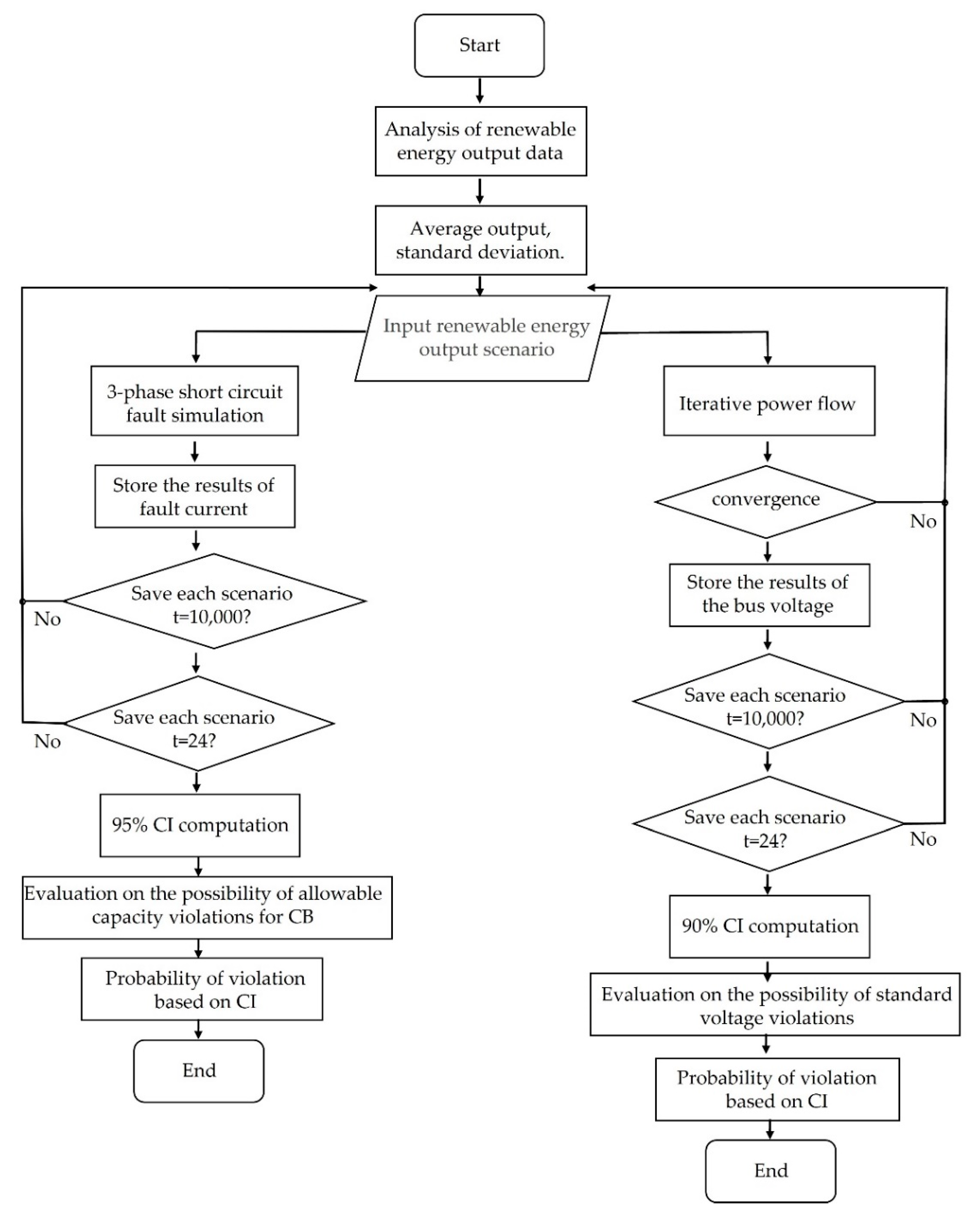
2. Proposed Methodology

In this study, a probabilistic stability evaluation methodology based on a confidence interval is presented and an algorithm for this is presented in Figure 1. First, various renewable energy output scenarios were implemented to complement the limitations of stability evaluation techniques through deterministic prediction. The number of renewable energy output scenarios selected by the user was used as the input data for the probabilistic stability evaluation. However, 10,000 output scenarios were generated in this study. Furthermore, iterative power flow and fault current calculation algorithms were applied to the two probabilistic stability evaluations. The confidence interval was computed based on the bus voltages and fault currents derived using each algorithm. After computing the cumulative distribution function based on the results for each parameter, we determined whether the stability is violated based on the distribution system stability index selected in this study. In this study, the allowable bus voltages and circuit breaker breaking current ratings were selected as indicators of the violation of stability in the distribution system.

2.1. Confidence Interval Computation

It may not be possible to accurately determine whether the stability that may occur is violated because the deterministic prediction technique does not consider the output variability of the RES. However, calculating the confidence interval based on various output scenarios could solve the problems of the deterministic prediction techniques. The confidence interval could be calculated using normal or cumulative distribution functions based on parameters such as the output, bus voltage, and fault current.
Figure 2 shows the calculation results of the confidence intervals using each function. Figure 2a shows the 90% CI based on the normal distribution function of the input variable of 5 and 95%. Similarly, Figure 3b presents the 90% CI based on the cumulative distribution function of the input variable of 0.05 and 0.95. The range of each section, having an input variable with an hourly cumulative distribution function of 0.05 and an input variable of 0.95, may be expressed as a confidence interval of 90%. Similarly, the range between the point where the cumulative distribution function is 0.45, and the input variable at the point where the cumulative distribution function is 0.55, can be expressed as a confidence interval of 10%. Additionally, the actual output value was assumed to be the result value based on the deterministic prediction technique, as shown in Figure 3b and Figure 4b. Thus, because the deterministic prediction technique does not consider the variability of renewable energy, it may not have been possible to determine whether the stability that may occur is violated accurately. However, calculating the confidence interval based on various output scenarios overcame the limitations of deterministic prediction techniques. In advance, it could be determined whether the actual output was included within a specific confidence interval.

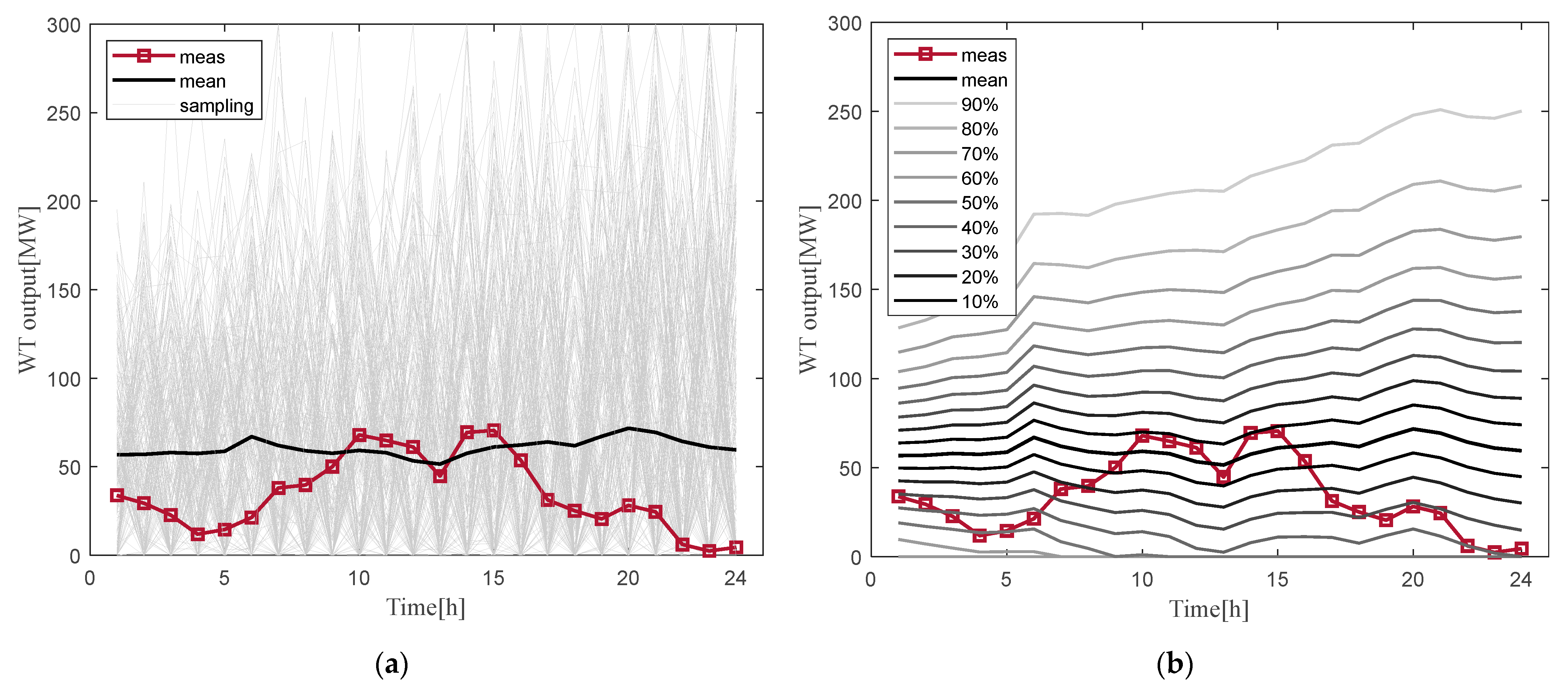
2.2. Implementation of Renewable Energy Output Scenario

In this section, a scenario creation method is presented. First, historical data of renewable energy output were analyzed for probabilistic stability evaluation. In this study, PV and WT output data from Jeju Island from January to June 2021 were used. Second, the normal distribution function was derived using the average (μ) and standard deviation (σ) of the hourly output as the parameters. The formula below is a probability density function equation that represents a normal distribution. Third, based on the aforementioned factors, renewable energy output scenarios were generated by sampling and were used as input data for the system analysis models. The scale of the output scenario was adjusted to proceed with a case study suitable for a systematic situation. Finally, this study analyzed the possibility of violations of allowable bus voltages and circuit breaker breaking current ratings using the confidence intervals of bus voltages and fault currents.
f ( x ) = 1 σ 2 π e ( x u ) 2 2 σ 2
Figure 3a shows the PV output scenario with the actual and average outputs. The PV output had a convex bell shape and showed similar patterns daily because it was only generated during the day. Figure 3b presents the profile obtained by calculating the confidence interval based on the results of the PV output. The uncertainty of the actual output was evaluated by calculating the confidence interval. In the figures, the term ‘meas’ means the result of applying the actual RES output profile, and the term ‘mean’ represents the average of RES output every hour.
The WT output scenario is shown in Figure 4a. The WT output exhibited irregular and highly volatile characteristics. Additionally, in Figure 4b, the confidence interval computed using the cumulative distribution function based on the wind power output is shown. However, in this study, the confidence interval was not calculated based on the renewable energy output scenario as shown in Figure 3b and Figure 4b. After applying 10,000 output scenarios to the test model, the stability was evaluated by calculating the confidence interval based on the bus voltage and fault current results. The output scenario was reflected in the probabilistic stability evaluation through this procedure. In this study, it was used as the input data for probabilistic voltage stability evaluation and fault analysis.

2.3. Iterative Power Flow Algorithm

This section considers iterative power flow algorithm to evaluate the probabilistic voltage analysis. In this paper, renewable energy output scenarios were entered and the Newton–Raphson method was applied. The Newton–Raphson method is an algorithm that precisely calculates the approximation of high-order nonlinear equations through iterative equations.
f ( x ) = f ( a ) + f ( 1 ) ( a ) ( x a )
If the initial value a is xi in this approximation, this approximation can be represented as follows.
f ( x ) = f ( x i ) + f ( 1 ) ( x i ) ( x x i )
The solution can be obtained by making the above approximation zero. If the approximation derived from applying xi is xi+1, the error is equal to | x i + 1 x i | . This is repeated until the error is less than the specified error. Here, f 1 ( x , y ) ,   f 2 ( x , y ) expand the Taylors Series formula, respectively.
f 1 ( x i + 1 ,   y i + 1 ) = f 1 ( x i ,   y i ) + f 1 x ( x i ,   y i ) ( x i ) + f 1 y ( x i ,   y i ) ( y i ) = 0 f 2 ( x i + 1 ,   y i + 1 ) = f 2 ( x i ,   y i ) + f 2 x ( x i ,   y i ) ( x i ) + f 2 y ( x i ,   y i ) ( y i ) = 0
To find a solution to the higher-order nonlinear equation, we left the right side of the Taylor series at zero. The above equation can be expressed as a vector product as follows.
[ f 1 ( x i ,   y i ) f 2 ( x i ,   y i ) ] + [ f 1 x   f 1 y f 2 x   f 2 y ] [ x i y i ] = 0
Here, the Jacobian matrix j is defined as follows.
j = [ f 1 x   f 1 y f 2 x   f 2 y ]
And x i ,   y i are defined as follows.
x i = x i + 1 x i y i = y i + 1 y i
The initial value x i , y i is a known value, and x i + 1 , y i + 1 is a value to be obtained. If x i + 1 , y i + 1 are placed on the left side, it is summarized as the following equation.
[ x i + 1 y i + 1 ] = [ x i y i ] [ f 1 x   f 1 y f 2 x   f 2 y ] 1 [ f 1 ( x i ,   y i ) f 2 ( x i ,   y i ) ]

2.4. Fault Current Analysis Algorithm

This section presents fault current analysis algorithm to evaluate the probabilistic fault current analysis. In the case study of this paper, the three-phase short-circuit fault was applied for the simulation of the worst-case situation. The conditions of the voltage and current in each phase are as follows.
  I a + I b + I c = 0   V a + V b + V c = 0
where Ia, Ib, and Ic are the phase-A, -B, and -C currents, respectively. Here, Va, Vb, and Vc are the phase-A, -B, and -C voltages, respectively. Then, Equation (11) represents the sequence components of the fault voltage.
V 0 = Z 0 I 0 = Z 0 3 (   I a + I b + I c ) = 0 V 1 = 1 3 ( V a + a V b + a 2 V c ) = 1 3 ( 1 + a + a 2 )   V a = 0 V 2 = 1 3 ( V a + a 2 V b + a V c ) = 1 3 ( 1 + a 2 + a )   V a = 0
where V1, V2, and V0 are the positive-, negative-, and zero-sequence voltages, respectively. Then, Equation (5) represents the sequence components of the fault voltage. This formula can be summarized as follows.
V 0 = Z 0 I 0 = 0       I 0 = 0 V 1 = E a Z 1 I 1 = 0       I 1 = E a Z 1 V 2 = Z 2 I 2 = 0       I 2 = 0
Accordingly, the short-circuit current of each phase may be expressed using the following equation.
I a = I 0 + I 1 + I 2 = I 1 = E a Z 1 I b = I 0 + a 2 I 1 + a I 2 = a 2 E a Z 1 I c = I 0 + a I 1 + a 2 I 2 = I 1 = a E a Z 1

3. Case Study

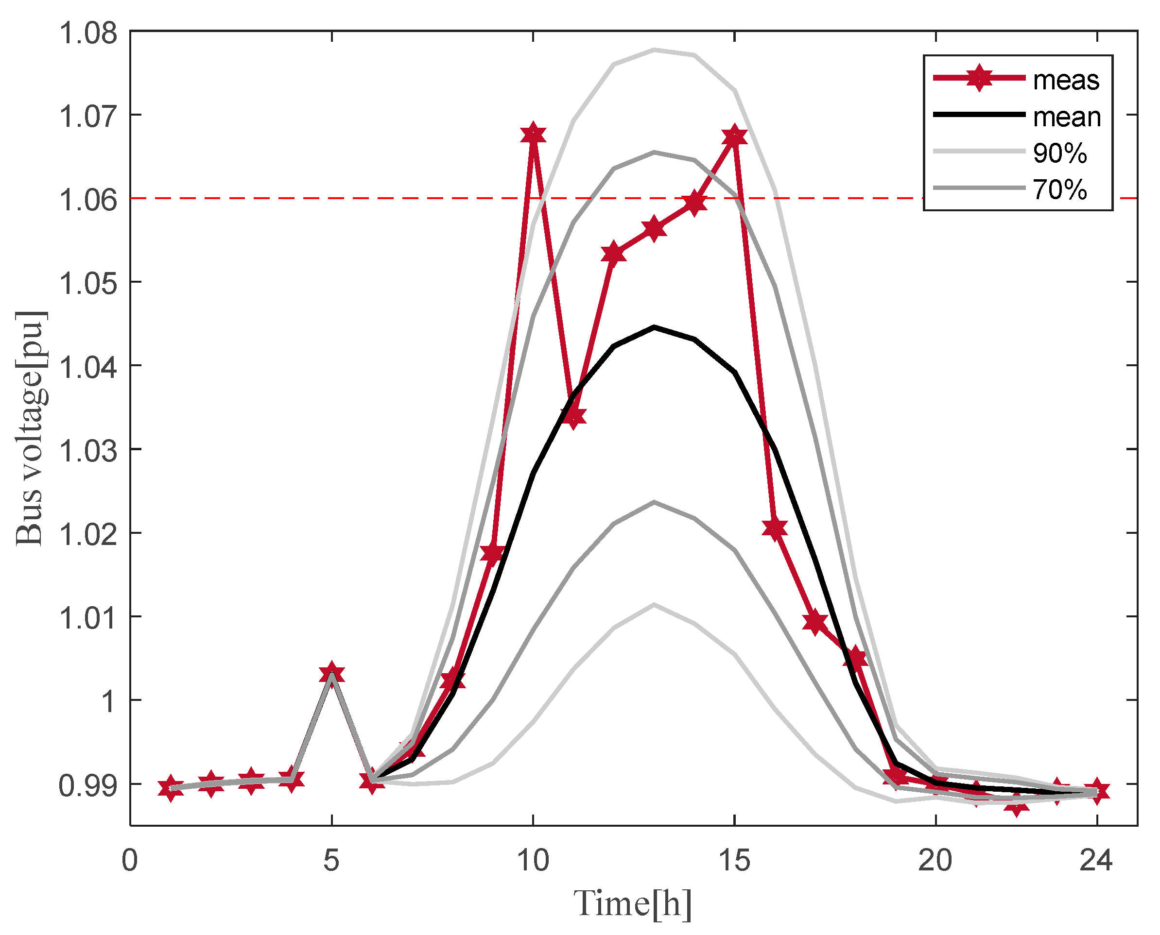
3.1. Probabilistic Voltage Stability Analysis

First, various renewable energy output data were implemented and used as the input data for the system analysis model. An iterative power flow was applied to evaluate probabilistic voltage stability. By analyzing the steady state and calculating the confidence interval based on the bus voltage result, we evaluated whether it exists within the standard voltage range.

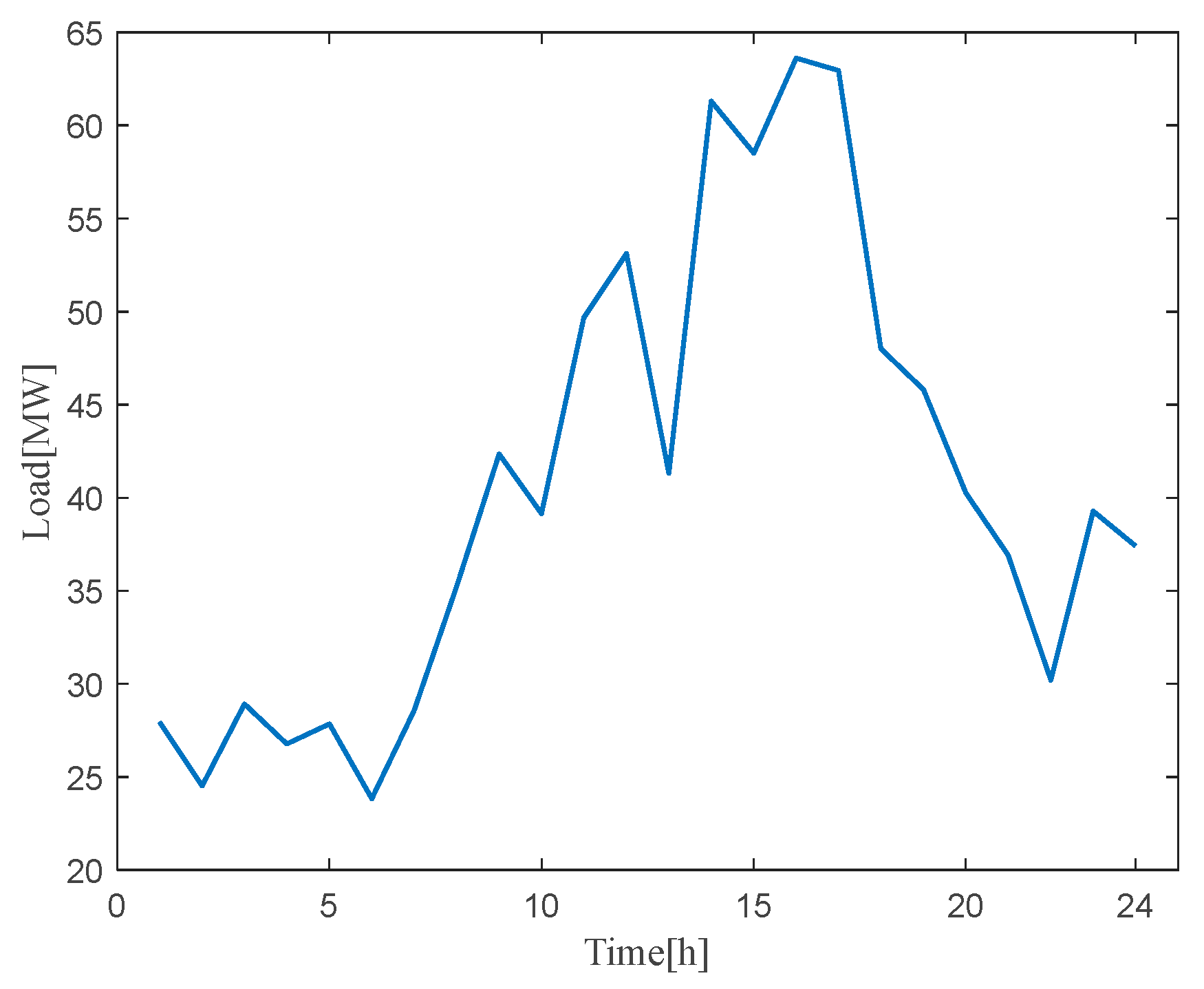
3.1.1. Test System Setup for Probabilistic Voltage Analysis

Generally, ‘voltage stability’ refers to the ability of a power system to allow all bus voltages to remain within the standard voltage range after a disturbance from the initial operating conditions occurs. However, the ‘voltage stability’ in this study indicated a standard voltage violation in the reliability criterion. According to the performance standard of electrical equipment for the distribution of KEPCO, the standard voltage range in the low-voltage distribution system was specified as shown in Table 1. This section examines the possibility of violating the standard voltage of a low-pressure distribution system based on various renewable energy output scenarios.
The renewable energy output scenario implemented using MATLAB was reflected in the test system. Figure 5 presents a KEPCO standard distribution system consisting of a main generator, MTR, loads, recloser, interconnection transformer, and inverter-based DG. Table 2 presents rated powers and voltages of each component. Figure 6a,b show the PV output and load profile, respectively. PV had the highest output at 1 p.m., and the load decreased during the day but gradually increased in the evening.
The case study considered that grid integration of renewable energy would continue to increase in the future. Additionally, the ratio of the total facility capacity of the PV to load of the day was assumed to be 24:5 to evaluate the worst-case scenario for voltage stability. The test system had eight PVs with a capacity of 3 MW and five loads with a capacity of 1 MW.
The results of the bus voltage for the number of output scenarios for 24 h were stored as a matrix (10,000 × 24) using the power flow calculation algorithm. In the subsequent section, the confidence interval calculated based on the bus voltage results and the probabilistic analysis performed to determine whether the standard voltage is violated hourly are presented.

3.1.2. Probabilistic Voltage Analysis Based on CI

The confidence interval was calculated based on the bus voltage results to evaluate whether the standard voltage was violated. Figure 7 shows the voltage results for the 31-bus system. In the box plot, the base and upper side of the blue box represent the bus voltage when the cumulative distribution function is 15% and 85%, respectively. Thus, the area of the blue box can be expressed as a confidence interval of 70%. Therefore, assuming that the red line in the blue box is a deterministic prediction result obtained by inputting the actual output, it was not possible to determine whether the standard voltage is violated. However, the standard voltage violation case could be determined by computing a confidence interval of 70% based on various output scenarios. Table 3 lists the maximum voltage and the probability of violation of the 31-bus voltage. Consequently, overvoltage occurred from 10 a.m. to 4 p.m., and overvoltage occurred at approximately 30% probability at 1 p.m. when the solar power output fluctuations were severe.
Figure 8 shows the voltage results for the 31-bus and Table 4 shows the overvoltage ratio to the 90% confidence interval. Outliers that could not be confirmed through the box plot were analyzed by calculating the confidence interval at 90%. Additionally, when the distribution system operator calculated a confidence interval of 70%, there was an economic margin in terms of system design and operation. However, there was a possibility of violating the stability in the section outside the predicted range. Conversely, when the confidence interval was high, more results could be considered and stability violations could be evaluated in detail. Compared with the low confidence interval, the system should be designed and operated considering the risk section that violates the standard voltage.
Figure 9 shows the voltage results for the eight-bus voltage and Table 5 presents the overvoltage ratio to the 90% confidence interval. The results of the eight-bus voltage were compared with those of the 31-bus voltage. When calculating the confidence interval in the 70% section, all voltages were within the standard voltage range unlike the result of the 31-bus voltage. Moreover, when the confidence interval was calculated as 90%, overvoltage occurred, and violations compared with the confidence interval were within approximately 30%.
Finally, Figure 10 shows the confidence interval profile for the 24-bus voltage and Table 6 presents the probabilistic analysis. The time when overvoltage occurred was the same as that of the eight-bus voltage; however, the ratio of violation cases to the confidence interval was slightly higher. Moreover, in the eight-bus voltage, it was included within the standard voltage range in the 70% confidence interval, representing the interval between the voltage with the cumulative distribution function of 0.15 and a voltage of 0.85. However, the 24-bus voltage was not within the standard voltage range.
The possibility of a violation of the standard voltage in the distribution system connected to the PV system was examined, and it was discovered that the standard voltage was violated according to the PV variability. Particularly, the probability of standard voltage violations increased during the day when the PV output rapidly increased. Accordingly, the variability problem may adversely affect the load-side or power facility.

3.2. Probabilistic Fault Analysis

In this study, various output data were implemented and used as the input data for the system analysis model. The confidence interval was calculated based on the result of the fault current after the three-phase short-circuit fault to evaluate whether it existed within the allowable capacity range of the circuit breaker (CB).

3.2.1. Test System Setup for Probabilistic Fault Analysis

Figure 11 shows the KEPCO standard distribution system with inverter-based DGs. The sequence impedances of the aerial lines are the actual values used in Korea. DGs were interfaced through six feeders, with DG 1–4 representing PV and DG 5–6 representing WT. Table 7 presents rated powers and voltages of each component. Additionally, Table 8 indicates the rated breaking current of the CB for the 22.9 kV distribution system. Based on various scenarios, it was examined whether the three-phase short-circuit current violates 12.5 kA.
The PV and WT output scenarios were reflected in the test system, as shown in Figure 11. Figure 12a,b represent the PV and WT output profiles, respectively, considering the allowable capacity of the DG for each feeder. Figure 13 shows the load profile.
This study implemented the test system above to review the maximum breaking current considering the variability and worst-case scenario in the distribution system connected to renewable energy. The ratio of the total facility capacity of the PV to load of the day was assumed to be 1:5. The test system had four PVs, two WT of 12 MW, and a load of 60 MW for each feeder.
The three-phase short-circuit fault current for the number of output scenarios for 24 h was stored as a matrix (10,000 × 24). As shown in the subsequent section, the confidence interval was calculated using the normal or cumulative distribution function based on the fault-current results; the violation of the allowable breaker capacity was examined hourly.

3.2.2. Probabilistic Fault Analysis Based on CI

Based on the results of the three-phase short-circuit fault current, the confidence interval was calculated to evaluate whether the allowable capacity of the CB was violated. Figure 14 shows the fault current, derived by reflecting the output scenario, in the form of a box plot. In a box plot, the base and upper side represent the fault current when the cumulative distribution function is 2.5% and 97.5%, respectively. So, the area of the blue box can be expressed as the 95% CI, and an outlier is defined as a red data point located outside of each box plot. Additionally, assuming that the short red line inside this blue box is a deterministic prediction result obtained by inputting the actual output, it would be impossible to determine whether the allowable capacity of CB was violated.
However, if a 95% confidence interval is computed, it can accurately identify cases that violate the allowable capacity of the CB. Table 9 lists the probability of violating the allowable capacity of the CB. Between 2 p.m. and 5 p.m., fault currents exceeding the allowable capacity occurred, and the probability of violation was the highest at 4 p.m., with a probability of approximately 14%.
Figure 15 shows the confidence interval profile for the fault current and Table 10 lists the probability of allowable capacity violation based on the 95% CI. In Figure 1, the confidence interval range was within the allowable capacity range when the confidence interval was 70%. An overcurrent occurred when the confidence interval was 95%. Accordingly, if the confidence interval is low, there may be cases of stability violations in the section outside the predicted range; therefore, it was necessary for the confidence interval to be high. Thus, when the 95% confidence interval was calculated, more cases could be considered; therefore, the worst-case situation and risk section could be evaluated in detail.
Figure 16 shows the limitations of deterministic prediction techniques. Table 11 represents the comparison table of fault current results of the actual output profile. As a result, the risk section that cannot be identified through deterministic prediction could be determined using the proposed methodology. Moreover, based on the CI calculated by the distribution system operator (DSO), it was possible to determine the probability of the actual output value in advance. For example, measurements one and two were outside the range predicted to be 95%, resulting in a violation of the allowable capacity, and measurement three was within the range predicted to be 95%. Because the deterministic technique predicts a specific output value, it may not have been possible to determine a stability violation case. However, by computing CI, the possibility of a stability violation could be preemptively determined. Thus, it was possible to examine in advance the percentage of the actual output value that is included within the confidence interval. Additionally, through the proposed methodology, the DSO could be used as an indicator for decision making on how to establish the distribution system operation.
The possibility of a violation of the rated breaking current was examined in the case study, and the allowable capacity was violated according to variability such as the power demand and variability in the distribution system connected to inverter-based DGs. Consequently, it is imperative to expand the acceptability of distributed power to ensure the stability of the distribution system. Furthermore, measures such as meeting low voltage ride through (LVRT) requirements, increasing short-circuit current rating, and reducing the fault current is required. Moreover, from the perspective of future power distribution system plans, it can be used to select the capacity of power distribution system breakers using the proposed methodology. Based on various output scenarios, it is possible to plan and invest in power distribution system facilities by reviewing the maximum rated breaking current according to the CI.

4. Discussions and Conclusions

This study proposed a probabilistic stability evaluation method based on CI in distribution systems with inverter-based distributed generation. The proposed methodology could preemptively identify stability violations that may occur in the future. Further, the feasibility of the proposed methodology was demonstrated by predicting relatively accurate risk sections that could not be predicted using deterministic prediction techniques. Finally, the proposed methodology can be used by distribution system planners to establish appropriate mitigation measures and facility plans. The important points that should be considered in terms of operation and design may vary because the DSO calculates the CI.
The primary limitation in the analysis of stability violation was that the deterministic methodology cannot consider the variable nature of renewables. Therefore, it was necessary to determine the possibility of stability violation based on probabilistic scenarios. Based on the historical renewable energy output data, 10,000 output scenarios were generated and used as input data for probabilistic stability evaluation. An iterative power flow calculation algorithm was used for the probabilistic voltage stability evaluation, and a symmetric component circuit that considers imbalanced components was used for probabilistic fault analysis. At this time, the inverter-based DG was implemented with a current source that supplied a fault current that was smaller than the rated current and Norton equivalent impedance by a value of 1–1.2. This study analyzed the possibility of violations of allowable bus voltages and circuit breaker breaking current ratings using the confidence intervals of bus voltages and fault currents.
The primary findings of this study can be summarized as follows.
  • Performing a steady-state analysis in the distribution system to which PV is connected, the probability of violating the standard voltage during the daytime when PV fluctuations are severe was the highest.
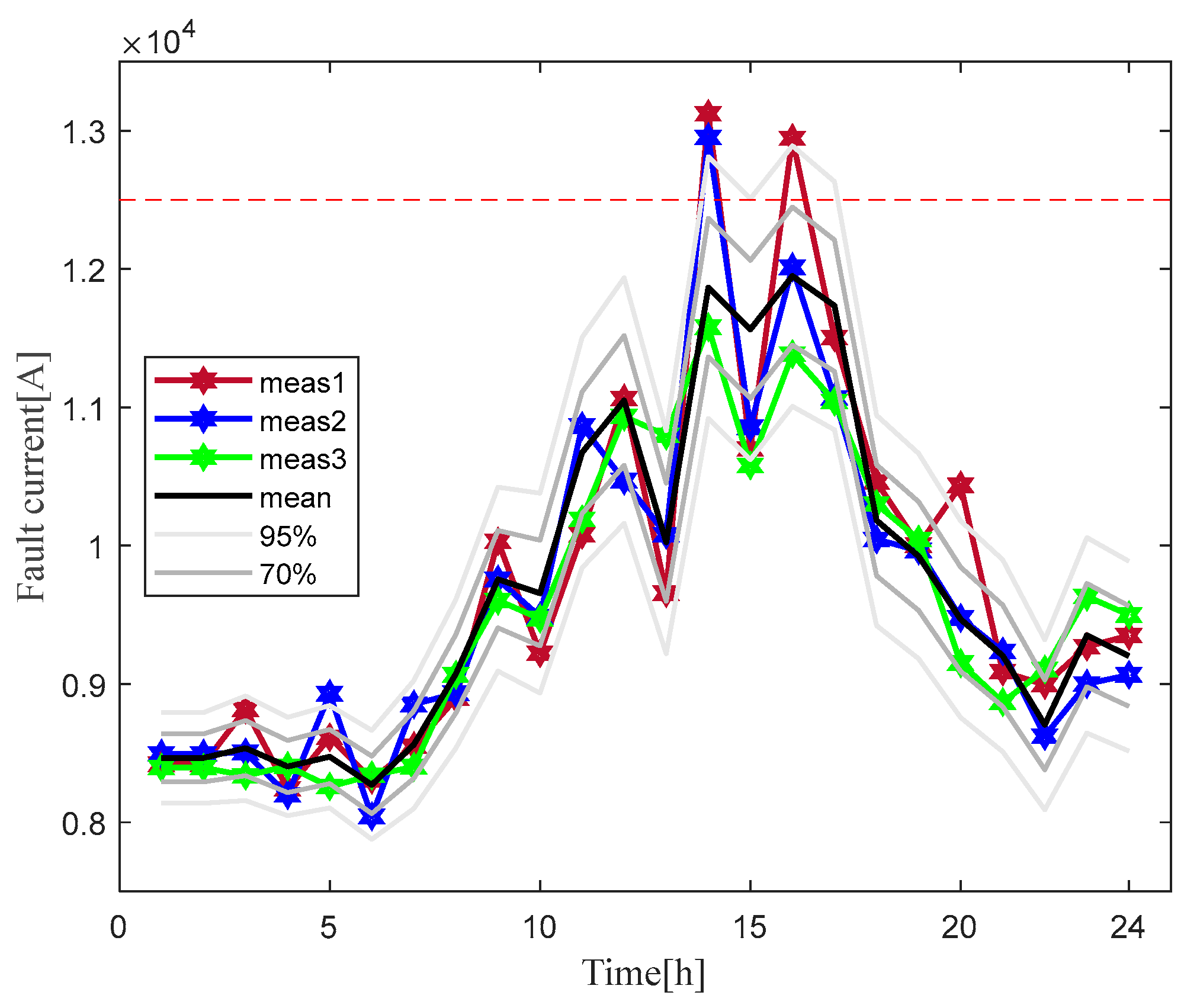
  • Because of the simulation of a three-phase short-circuit in the distribution system that is connected to the PV and WT, it was discovered that it could violate the allowable capacity of the CB owing to the effects of the power demand pattern and output variability.
The recent machine-learning techniques can improve the prediction accuracy of renewable energy output, by which the proposed method can produce more credible stability analysis results.

Author Contributions

Conceptualization, M.L., M.Y. and S.C.; data curation, M.L. and M.Y.; formal analysis, M.L.; funding acquisition, S.C.; investigation, S.C.; methodology, M.L.; project administration, J.C. and S.C.; resources, J.C.; software, M.Y.; supervision, S.C.; validation, M.L., M.Y. and S.C.; visualization, M.L. and S.C.; writing—original draft, M.L.; writing—review and editing, M.L. and S.C. All authors have read and agreed to the published version of the manuscript.

Funding

This research was supported in part by the KEPCO Research Institute under the project entitled by “A Research of Advanced Distribution Planning System for Mid-long term (R20DA16)”, in part by the Human Resources Program in Energy Technology of the Korea Institute of Energy Technology Evaluation and Planning (KETEP) and the Ministry of Trade, Industry & Energy (MOTIE) of the Republic of Korea (No. 20204010600220), and in part by the Basic Research Program through the National Research Foundation of Korea (NRF) funded by the MSIT (No. 2020R1A4A1019405).

Institutional Review Board Statement

Not applicable.

Informed Consent Statement

Not applicable.

Data Availability Statement

Not applicable.

Conflicts of Interest

The authors declare no conflict of interest.

References

  1. Rakibuzzaman, S.; Mithulananthan, N. A review of key power system stability challenges for large-scale PV integration. Renew. Sustain. Energy Rev. 2015, 41, 1423–1436. [Google Scholar] [CrossRef]
  2. Ahmad, S.; Ahmad, A. A compendium of performance metrics, pricing schemes, optimization objectives, and solution methodologies of demand side management for the smart grid. Energies 2018, 11, 2801. [Google Scholar] [CrossRef] [Green Version]
  3. Kassia, M. California Duck Curve ‘Alive and Well’ as Renewable, Minimum Net Load Records Set. Cal-ISO. 2021. Available online: https://www.spglobal.com/commodity-insights/ko/market-insights/latest-news/electric-power/032621-california-duck-curve-alive-and-well-as-renewable-min-net-load-records-set (accessed on 15 February 2022).
  4. Chakraborty, N.; Mondal, A. Intelligent scheduling of thermostatic devices for efficient energy management in smart grid. IEEE Trans. Ind. Inform. 2017, 13, 2899–2910. [Google Scholar] [CrossRef]
  5. Muhammad, R.; Sadiq, A. Probabilistic Optimization Techniques in Smart Power System. Energies 2022, 15, 825. [Google Scholar] [CrossRef]
  6. Qamar, A.; Iqbal, S. Configuration Detection of Grounding Grid: Static Electric Field Based Nondestructive Technique. IEEE Access 2021, 9, 132888–132896. [Google Scholar] [CrossRef]
  7. Kundur, P.; Paserba, J. Definition and classification of power system stability IEEE/CIGRE joint task force on stability terms and definitions. IEEE Trans. Power Syst. 2004, 19, 1387–1401. [Google Scholar] [CrossRef]
  8. Mathur, A.; Das, B. Fault analysis of unbalanced radial and meshed distribution system with inverter based distributed generation. Int. J. Electr. Power Energy Syst. 2017, 85, 164–177. [Google Scholar] [CrossRef]
  9. Dukpa, A.; Venkatesh, B. Application of continuation power flow method in radial distribution systems. Electr. Power Syst. Res. 2009, 79, 1503–1510. [Google Scholar] [CrossRef]
  10. Ramadan, A.; Mohamed, E. Optimal power flow for distribution systems with uncertainty. In Uncertainties in Modern Power Systems; Academic Press: London, UK, 2021; pp. 145–162. [Google Scholar] [CrossRef]
  11. Carpinelli, G.; Lauria, D. Voltage stability analysis in unbalanced power systems by optimal power flow. IEE Proc.-Gener. Transm. Distrib. 2006, 153, 261–268. [Google Scholar] [CrossRef]
  12. Iranpour, M.; Hejazi, A. Probabilistic Voltage Instability Assessment of Smart Grid Based on Cross Entropy Concept. In Proceedings of the 2020 10th Smart Grid Conference (SGC), Kashan, Iran, 16–17 December 2020; pp. 1–6. [Google Scholar] [CrossRef]
  13. Wang, H.; Zheng, Y. Probabilistic power flow analysis of microgrid with renewable energy. Int. J. Electr. Power Energy Syst. 2020, 114, 105393. [Google Scholar] [CrossRef]
  14. Xiaoyuan, X.; Zheng, Y. Power system voltage stability evaluation considering renewable energy with correlated variabilities. IEEE Trans. Power Syst. 2017, 33, 3236–3245. [Google Scholar] [CrossRef]
  15. Wang, Y.; Vittal, M. Probabilistic reliability evaluation including adequacy and dynamic security assessment. IEEE Trans. Power Syst. 2019, 35, 551–559. [Google Scholar] [CrossRef]
  16. Yang, H.; Shi, X. Monitoring Data Factorization of High Renewable Energy Penetrated Grids for Probabilistic Static Voltage Stability Assessment. IEEE Trans. Smart Grid 2021, 13, 1273–1286. [Google Scholar] [CrossRef]
  17. Mohammed, A.; Kazi, N. Identification of Efficient Sampling Techniques for Probabilistic Voltage Stability Analysis of Renewable-Rich Power Systems. Energies 2021, 14, 2328. [Google Scholar] [CrossRef]
  18. Deng, W.; Buhan, Z. Risk-based probabilistic voltage stability assessment in uncertain power system. Energies 2017, 10, 180. [Google Scholar] [CrossRef] [Green Version]
  19. IEEE Std 1547.7; IEEE Guide for Conducting Distribution Impact Studies for Distributed Resource Interconnection. IEEE: Piscataway, NJ, USA, 2014. [CrossRef]
  20. Kim, I. Short-Circuit Analysis Models for Unbalanced Inverter-Based Distributed Generation Sources and Loads. IEEE Trans. Power Syst. 2019, 34, 3515–3526. [Google Scholar] [CrossRef]
  21. Wang, Q.; Zhou, N. Fault analysis for distribution networks with current-controlled three-phase inverter-interfaced distributed generators. IEEE Trans. Power Deliv. 2015, 30, 1532–1542. [Google Scholar] [CrossRef]
  22. Mirshekali, H.; Dashti, R. A novel fault location methodology for smart distribution networks. IEEE Trans. Smart Grid 2020, 12, 1277–1288. [Google Scholar] [CrossRef]
Figure 1. Probabilistic stability evaluation based on confidence interval.
Sustainability 14 03806 g001
Figure 2. CI computation: (a) normal distribution function; (b) cumulative distribution function.
Sustainability 14 03806 g002
Figure 3. Implementation for scenario: (a) PV output scenario; (b) PV output scenario based on CI.
Sustainability 14 03806 g003
Figure 4. Implementation for scenario: (a) WT output scenario; (b) WT output scenario based on CI.
Sustainability 14 03806 g004
Figure 5. Actual distribution system interfaced with PVs.
Sustainability 14 03806 g005
Figure 6. Parameter based on the test system: (a) PV output profile; (b) Load profile.
Sustainability 14 03806 g006
Figure 7. 31-bus voltage results of the box plot shape.
Sustainability 14 03806 g007
Figure 8. Result of 31-bus voltage based on 90% CI.
Sustainability 14 03806 g008
Figure 9. Result of eight-bus voltage based on 90% CI.
Sustainability 14 03806 g009
Figure 10. Results of 24-bus voltage based on 90% CI.
Sustainability 14 03806 g010
Figure 11. Actual distribution system interfaced with PVs and WTs.
Sustainability 14 03806 g011
Figure 12. Parameter based on the test system: (a) PV output profile; (b) WT output profile.
Sustainability 14 03806 g012
Figure 13. Load profile.
Sustainability 14 03806 g013
Figure 14. Fault current results of the box plot shape.
Sustainability 14 03806 g014
Figure 15. Results of fault current based on 95% CI.
Sustainability 14 03806 g015
Figure 16. The limitations of deterministic prediction techniques.
Sustainability 14 03806 g016
Table 1. Standard voltage range in the low-voltage distribution system.
Nominal VoltageStandard
Voltage Range (V)
Standard
Voltage Range (pu)
low voltage220207–233 (±13)207–233 (±1.06)
Table 2. System parameters of the test system set up for probabilistic voltage analysis.
Main Generator (G1)MTRLineInterconnection Transformer (T1)DG
Rated power [MVA]1004510033 (DG1, DG8)
Rated voltage [kV]154154/22.9/6.622.922.9/0.380.38
Table 3. Maximum voltage and probability of violation for the 31-bus voltage.
Violation TimeMaximum Voltage (V)Probability of Voltage Violation Based on Scenarios (%)
10 a.m.1.06754.05
11 a.m.1.067414.9
12 p.m.1.067525.97
1 p.m.1.067630.68
2 p.m.1.067428.66
3 p.m.1.067320.48
4 p.m.1.06716.65
Table 4. Probability of 31-bus voltage violation based on 90% CI.
Violation TimeVoltage Range for 90% CI (pu)Probability of Voltage Violation Based on 90% CI (%)
11 a.m.1.0037–1.069217.38
12 p.m.1.0086–1.07627.92
1 p.m.1.0139–1.077732.94
2 p.m.1.0091–1.077130.82
3 p.m.1.0055–1.072921.86
4 p.m.0.9989–1.0617.5
Table 5. Probability of eight-bus voltage violation based on 90% CI.
Violation TimeVoltage Range for 90% CI (pu)Probability of Voltage Violation Based on 90% CI (%)
11 a.m.1.0019–1.067414.9
12 p.m.1.0065–1.067525.97
1 p.m.1.009–1.067630.68
2 p.m.1.0069–1.067428.66
3 p.m.1.0036–1.067320.48
Table 6. Probability of 24-bus voltage violation based on 90% CI.
Violation TimeVoltage Range for 90% CI (pu)Probability of Voltage Violation Based on 90% CI (%)
11 a.m.1.0031–1.06713.6
12 p.m.1.0079–1.073625.22
1 p.m.1.0107–1.075329.99
2 p.m.1.0085–1.074730.68
3 p.m.1.0049–1.070518.92
Table 7. System parameters of the test system set up for probabilistic fault analysis.
Main Generator (G1)MTRLineInterconnection Transformer (T1)DG
Rated power [MVA]10045/15/151001212 (DG1, DG4)
12 (DG5, DG6)
Rated voltage [kV]154154/22.9/6.622.922.9/0.380.38
Table 8. Breaking capacity for CB in 22.9 kV distribution system.
Breaking Capacity Range (kA)
Rated breaking current 12.5 and/or below
Table 9. Maximum fault current and probability of allowable capacity violation.
Violation TimeMaximum Fault Current (kA)Probability of Allowable Capacity Violation Based on Scenarios (%)
2 p.m.13.46411.02
3 p.m.13.1753.98
4 p.m.13.70414
5 p.m.13.5527.17
Table 10. Probability of allowable capacity violation based on 95% CI.
Violation TimeFault Current Range for 95% CI (pu)Probability of Allowable Capacity Violation Based on 95% CI (%)
2 p.m.10.919–12.81211.62
3 p.m.10.62–12.5074.18
4 p.m.11.005–12.89114.57
5 p.m.10.837–12.6327.52
Table 11. Comparison of fault current results of actual output profile.
Application of Actual Output Profile Fault Current (kA)95% CI Violation Time
Measurement 1
[12 March 2021]
13.12
12.94
2 p.m.
4 p.m.
Measurement 2
[12 March 2021]
12.952 p.m.
Measurement 3
[12 March 2021]
--
Publisher’s Note: MDPI stays neutral with regard to jurisdictional claims in published maps and institutional affiliations.

